
Submitted:
07 June 2025
Posted:
09 June 2025
You are already at the latest version
Abstract
Crossland Tankers is a leading manufacturer of bulk-load road tankers in Northern Ireland. These tankers transport up to forty thousand litres of liquid over long distances across diverse road conditions. Liquid sloshing within the tank has a significant impact on driveability and the tanker's lifespan. This project develops a comprehensive LS-DYNA model to enhance the tanker design process and address these challenges. Due to environmental, financial, and time constraints, multiphysics simulations are becoming more prominent in the competitive manufacturing industry. This project aims to develop a general-purpose model of a road tanker that integrates road, tyre, and suspension dynamics alongside fluid-structure interactions, enabling a detailed analysis of various driving conditions. The approach uses OASYS PRIMER as a preprocessor for LS-DYNA, integrating Smooth Particle Hydrodynamics (SPH) to model fluid dynamics and Explicit Dynamic Finite Element (FE) techniques to model the chassis. The model simulates scenarios such as emergency braking to identify areas of high fatigue due to liquid load and sloshing. The validation was conducted through road testing with acceleration and strain data collected using a portable Data Acquisition device (DAQ). By integrating advanced material characterisation for 304 stainless steels with a robust Multiphysics model, this research provides a holistic approach for optimising tanker design for enhanced safety and performance.
Keywords:
Multiphysics
; Smooth Particle Hydrodynamics
; Finite element
; Chassis design
; structure dynamics
; fluid-structure interaction
; fluid sloshing
; accelerometers
; strain gauge
1. Introduction
Crossland Tankers began in 1988 as a tanker repair and service company but soon started manufacturing tankers for the UK road industry. Specialising in bulk liquid tankers, Crossland collaborates with customers from concept to completion to build tanks according to their requirements.
Bulk liquid transportation plays a significant role in the UK supply chain, with approximately 300 terminals dedicated to importing, exporting, and distribution. These tankers can travel hundreds of miles daily and are subject to forces that can severely impact the vehicle's lifespan and drivability, primarily road conditions and sloshing forces induced by the liquid.
Due to the varying quality of the UK's road network, both road conditions and how a vehicle is used can significantly shorten a tanker's lifespan. For instance, a milk collection vehicle often travels between farms on rough rural roads and at different fill levels. These factors can greatly impact the durability of the vehicle and its components if not properly considered during the engineering process.
Fluid Sloshing is the oscillatory motion of liquid inside a partially filled container due to external disturbances. In a road tanker, this can lead to safety concerns. Rapid braking or cornering can induce severe sloshing and destabilise a tanker by shifting the centre of gravity, increasing the risk of rollover.
For Crossland, a better understanding of the sloshing forces means they can make informed design choices and suggestions for improving the driveability and lifespan of the tanker. Designing a lightweight tanker allows for a greater payload, so the model will also be used to identify areas where weight reduction can be made without affecting the integrity of the tanker. This is an obvious selling point, as lightweight products offer more carrying capacity.
In today's manufacturing industry, there is a shift from physical prototyping to a greater emphasis on Multiphysics simulations, driven by advancements in computational capabilities and developments in simulation software. As these methods become more accurate and reliable, their presence in the design process will become increasingly prevalent, as virtual testing on numerous design iterations can be conducted at a fraction of the cost. Model validation must be performed to ensure accuracy by collecting real-world test data.
While current tools offer limited predictive accuracy for structural impacts of design changes, simulating a "worst-case scenario"—such as a tanker undergoing emergency braking—can help identify critical stress regions and assess how new design iterations affect structural integrity.
Figure 1 illustrates the comprehensive Multiphysics Tanker Model developed in this study. This model integrates various simulation domains essential for analysing the tanker's behaviour under realistic conditions, including SPH fluid modelling, FEA for the chassis, and suspension and road dynamics. The diagram highlights the approach's holistic nature, encompassing fluid-structure interactions (FSI) between the sloshing fluid, modelled with SPH, and the tanker structure, modelled with explicit dynamic Finite Element Analysis (FEA). This integration enables a comprehensive examination of the interactions between the fluid and the tanker's structural components under various driving scenarios. The SPH model, coupled with a robust suspension and road dynamics representation, provides a dynamic view of the fluid sloshing and its impact on the tanker's stability and structural integrity.
Additionally, SPH facilitates the modelling of fluid-structure interactions more effectively than traditional meshed methods. The penalty-based contact algorithms in SPH allow for accurate modelling of forces and stresses induced by fluid sloshing as the fluid interacts with tank walls and internal structures. Although SPH faces limitations in defining certain boundary conditions, such as inlets and outlets, this is not an issue in our sealed-tanker environment, making SPH a particularly suitable choice for this application. Xu et al. [3] compare ALE to SPH, concluding that while SPH avoids the heavy task of meshing, it may require finer resolution for accuracy, which can be offset by parallelisation techniques such as MPP in LS-Dyna. Previous applications of SPH to sloshing, as reported by Delorme et al. [4], Landrini et al. [5], and Chen et al. [6], have validated impact pressures using SPH in forced roll conditions. Nonetheless, Jonsson et al. [7] highlight that SPH resolution and artificial viscosity constants are key to reducing the error margin between experimental and numerical results, which often vary between 15% and 20%.
The kernel function W(r, h) serves as the cornerstone of SPH, weighting the contributions of neighbouring particles based on their distance r from a reference particle, with h being the smoothing length. The kernel function is defined as:
This function smooths out particle interactions, enabling the computation of continuous field variables such as density, pressure, and velocity from discrete particles. The interpolation of a field quantity A (density, pressure, or velocity) at a position r is given by the equation:
Where mj is the mass of particle j, ρj is the density of particle j, and rj is the position of particle j. This interpolation is crucial for representing continuous field quantities from discrete particle data, ensuring smooth and accurate simulations of fluid properties.
The kernel function W(r, h) and the interpolation equation A(r) are foundational to the SPH method, enabling the representation of continuous fluid properties from discrete particle data. The governing equations – continuity, momentum, and energy – describe how these properties evolve, utilising the kernel function and interpolation to ensure smooth and accurate simulations of fluid dynamics, particularly in scenarios involving complex interactions like fluid sloshing.
The continuity equation in SPH form is used to ensure mass conservation in the fluid. It calculates the rate of change of density for each particle based on the relative velocities of neighbouring particles. The continuity equation is expressed as:
Where ρi represents the density of particle i, vi and vj are the velocities of particles i and j, respectively, and ∇iW is the gradient of the kernel function concerning the position of particle i. This formulation calculates how the density of each particle changes over time, maintaining the correct mass distribution in fluid sloshing simulations.
The momentum equation governs the motion of fluid particles by accounting for forces acting on them, including pressure gradients and external forces. This equation is essential for calculating the acceleration of each fluid particle due to these forces and is given by:
In this equation, vi denotes the velocity of particle i, Pi and Pj are the pressures of particles i and j, ρi and ρj are the densities of particles i and j, and fi is the external force per unit mass on particle i. The summation of pressure contributions from neighbouring particles, weighted by ∇iW calculates the resultant force and subsequent acceleration on each particle, modelling how fluid particles move under various forces.
The energy equation in SPH tracks the internal energy changes of fluid particles, ensuring energy conservation. It calculates the change in internal energy due to work done by pressure forces and is represented by the equation:
In this equation, ui is the specific internal energy of particle i, Pi is the pressure of particle i, and ρi is the density of particle i. The summation of velocity differences from neighbouring particles, weighted by ∇iW, represents the energy exchange between particles. This equation helps model temperature and energy changes in the fluid, contributing to accurate predictions of fluid behaviour under dynamic conditions.
Explicit dynamic analysis is employed to simulate the transient response of the tanker's structure under dynamic loading conditions, including fluid sloshing and braking.
Where M is the mass matrix, C is the damping matrix, K is the stiffness matrix, u is the displacement vector, u˙ is the velocity vector, u¨ is the acceleration vector, F is the external force vector.
The coupling is achieved through fluid-structure interaction algorithms that allow for the transfer of forces and displacements between the fluid (SPH) and the structure (FEA). This bidirectional interaction ensures that the effects of fluid motion are accurately reflected in the structural response and vice versa. The penalty-based contact algorithm in LS-DYNA is used to model the interactions between the fluid particles and the tank walls:
Where Fcontact is the contact force, kp is the penalty stiffness, and δ is the penetration depth.
The integration of SPH and explicit FEA within LS-DYNA involves the following steps:
Initialisation: Define the initial conditions and properties for both the fluid (SPH particles) and the structure (FEA elements).
Simulation: Perform the simulation, where the SPH and FEA solvers run concurrently, exchanging data at each time step.
Data Exchange: Use coupling algorithms to transfer force and displacement data between the SPH and FEA models.
Post-Processing: Analyse the results to understand the interaction effects and validate the model against experimental data.
The novelty of our study lies in the comprehensive application of SPH in tandem with explicit dynamic FEA to accurately model and validate the complex fluid-structure interactions within road tankers. In contrast to prior studies that focused on simplified or isolated aspects of sloshing, this research integrates a full-scale Multiphysics simulation encompassing fluid behaviour, the tanker structure, suspension dynamics, and road interactions. This approach, validated through extensive real-world testing, provides critical insights into the structural integrity and driveability of road tankers under realistic conditions. By coupling advanced material characterisation techniques with a model of 304 stainless steel under high-cycle fatigue, our study delivers enhanced realism and applicability for improved tanker design and safety. This integrated framework not only sets a benchmark for future research but also offers practical applications for optimising tanker design to withstand dynamic operational stresses.
2. Methodology
2.1. Use of Smooth Particle Hydrodynamics (SPH) for Fluid Modelling
Several software tools were used to develop the tank model, which served as the foundation for creating the entire Multiphysics model. Firstly, Crossland uses Creo Parametric to create their CAD models. This program includes specific functions for designing parts from sheet metal, enabling the user to fold and unfold parts to verify manufacturability.
As any FEA engineer knows, meshing is often the most critical stage in the analysis process. Since the tank and chassis being studied are constructed from thin folded sheet metal, the problem is best tackled by meshing the structure as shells. ANSA from BETA CAE was chosen as the preprocessor for meshing the parts, as its batch processing and mid-surface extraction tools proved critical to the efficiency and quality of the 2D mesh extracted from 3d CAD geometry.
Once the parts had been meshed, OASYS PRIMER created the Ls-Dyna model. The OASYS suite offers excellent pre-, post-, and job submission tools, which I found helpful in interpreting and presenting results.
A simplified model of a rigid tank filled with water was created, as shown in Figure 2:
The tank was treated as a constrained, rigid structure, providing a reference frame for analysing its fluid dynamics. To simplify the forces experienced during real-world scenarios, a constant acceleration field of 3.5 m/s² was applied to the fluid. This acceleration mimics the effects of rapid deceleration or braking, which are critical conditions for evaluating sloshing behaviour.
The SPH particles were generated within the tank to a 60% fill level, which was chosen to reflect typical operating conditions with significant sloshing effects. According to the literature, achieving high resolution in SPH simulations is essential for accurately capturing the fluid's intricate flow features and dynamic interactions. Therefore, a parametric study was conducted to investigate the effects of various particle resolutions and artificial viscosity parameters on the simulation results.
Artificial viscosity is a crucial parameter in SPH simulations, as it helps stabilise the numerical solution and prevent unphysical oscillations in the fluid. We varied the artificial viscosity parameters to determine the optimal values and compared their effects on the simulation outcomes. Figure 3 illustrates the results of this parametric study, showing how different artificial viscosity settings impact the free surface features of the fluid.
Through this parametric analysis, we identified the most appropriate artificial viscosity parameters for various resolutions that balance computational efficiency and the accurate representation of fluid behaviour.
The maximum horizontal sloshing force was normalised using the default artificial viscosity values for the highest resolution case, as shown in Figure 4. This normalisation was necessary to facilitate a meaningful comparison across different resolutions. Since the highest-resolution case is expected to provide the most accurate representation of free-surface features, it serves as the benchmark for evaluating the effects of varying artificial viscosity parameters.
Our analysis revealed that as the SPH resolution lowers, the fluid produces a higher peak force and becomes more viscous. Setting the artificial viscosity constants to q1 = 1 and q2 = 1 resulted in a significantly lower sloshing force and less viscous fluid behaviour across all particle resolutions. This indicates that the choice of q2 has a more pronounced impact on the fluid's viscosity than q1. Based on the studies [X], we assume that the default values of q1 = 1.5 and q2 = 0.06 for the highest resolution case best reflect real-life conditions. Therefore, adjusting the artificial viscosity parameters to q1 = 1 and q2 = 1 at lower resolutions can yield comparable results. This adjustment compensates for the reduced resolution by enhancing the damping effects, thereby maintaining the accuracy of the simulation. The parametric study underscores the importance of fine-tuning artificial viscosity parameters to achieve realistic fluid behaviour in SPH simulations. A compromise must be made between particle resolution and computation time, and this study suggests optimal viscosity settings to mitigate the effects of lowering resolution.
2.2. Fluid-Structure Contact Algorithm
Within LS-DYNA, a penalty-based contact algorithm is used to model the interactions between the fluid and the interior surfaces of the tank. This type of contact algorithm has been extensively studied, with comprehensive details available in the work of Belytschko et al. [8]. The penalty-based approach is highly versatile and capable of handling both implicit and explicit analyses, making it particularly suitable for our general-purpose fluid-structure interaction model.
A penalty-based contact algorithm calculates the interaction force based on the penetration depth between contacting bodies. When two surfaces come into contact, the algorithm introduces a virtual spring between the nodes (agent nodes) of one body and the nearest surface segment (the master segment) of the other body. The contact force exerted by these virtual springs is proportional to the penetration depth, thereby preventing excessive overlap of the contacting surfaces. This method offers a realistic and computationally efficient approach to modelling complex interactions between fluid particles and tank walls.
Using linear springs to represent contact forces ensures the algorithm can accommodate various scenarios, from gentle fluid-wall interactions to more intense impact events. This flexibility is crucial for accurately simulating the dynamic behaviour of fluids within a tanker, where the interactions between the fluid and the tank structure can vary significantly depending on driving conditions and fill levels.
2.3. Challenges and Limitations
The simulated tank is 9 meters long and 2 meters in diameter. Given the substantial size of the tank, it is necessary to strike a balance between achieving a high enough resolution to accurately capture the flow features and maintaining a feasible computational run time. This trade-off is crucial for ensuring that the simulations are both accurate and computationally efficient. For our simulations, we aim to implement a two-way contact algorithm that checks the penetration of nodes bidirectionally. This means that the interactions between the fluid particles and the tank walls are dynamically updated in both directions, enhancing the realism of the simulation. However, this approach significantly increases the computational load. Specifically, the total CPU time spent on SPH calculations and their respective contact algorithms can be considerable, accounting for approximately 25-40% of the total computational time for the full tanker model, depending on the chosen SPH resolution.
Our primary interest lies in capturing the broader dynamics of the free surface within the tank and understanding its impact on its structural integrity. While extreme resolution is not necessary for visualising minute details of the free surface features, it is essential to achieve sufficient resolution to accurately represent the overall behaviour of the fluid and its interactions with the tank structure. Therefore, a balance must be found between these two factors to optimise the simulation's accuracy and efficiency. Simulating a large tank poses a significant challenge, necessitating careful consideration of resolution and computational feasibility. By focusing on the significant dynamics of the free surface and structural effects, we can ensure that our simulations provide valuable insights while effectively managing the computational demands.
2.4. FE Techniques for Chassis Modelling
The Full Tanker Assembly is exported from Creo as a .step file and imported into ANSA. The Mid Surface Extraction tool batch processes the 3d model assembly into a 2D shell mesh. The middle plane of each sheet metal part is extracted and then meshed as shells according to the specified mesh criteria. Each part has the thickness applied to every shell, allowing for the capture of changes in thickness within the geometry. These sheet metal parts are welded together during construction, potentially represented by hundreds of tied connections.
Using the Weld parts feature, this tool can be set up to batch process an entire assembly, allowing any parts within a certain distance tolerance to be "welded" together and defeatured of any unwanted holes or notches in the part geometry, as shown in Figure 5. The edges of each part are extended together, effectively forming a single part with shared nodes. With around 100 parts in the assembly, this proved a fast and effective way to represent the joints without defining *TIED_NODES_TO_SURFACE contacts between each part.
In conclusion, utilising ANSA for surface extraction, meshing, and part welding provides a quick and efficient method for preparing the complete tanker assembly for finite element analysis. This streamlined process ensures that the complex geometry of the tanker chassis is accurately represented, enabling a detailed and dependable structural analysis.
2.5. Suspension Elements
The axle operates on a suspension arm that pivots on a hanger mounted to the bottom of the chassis. An airbag spring and a damping arm are connected to the arm and the chassis, respectively, via the hanger. Together, they provide the essential suspension characteristics.
An axle manufacturer has provided key parameters for the suspension elements: a spring stiffness (k) of 150,000 N/mm and a damping coefficient (c) ranging from 10,000 to 50,000 N/mm² for both compression and tension. The finite element model represents the spring and damper elements using beam elements with the material model MAT_074 (ELASTIC_SPRING_DISCRETE_BEAM) and element formulation ELFORM = 6 (DISCRETE Beam). As shown in Figure 6, this representation enables the direct incorporation of the manufacturer-provided stiffness and damping values into the simulation. This ensures that the dynamic response of the suspension system is accurately captured.
The tyre was included as a linear spring-damper element, positioned between the axle and the road surface, to enhance the model's realism further. This addition simulates the tyre's cushioning effect and contribution to the overall suspension dynamics. Future validation of this part of the model can be achieved by using accelerometer data collected directly from the axle and the chassis above it. By comparing the simulated responses with real-world measurements, we can fine-tune the model to ensure it accurately reflects the physical behaviour of the suspension system.
3. Material Characterisation
304 Stainless Steel Used by Crossland
S304 Stainless Steel is utilised within tanker chassis and certain structural components. Consequently, accurately characterising this material is crucial to ensuring the reliability and performance of the tankers. The manufacturing process involves laser-cutting large sheets of S304 Stainless Steel, which are then folded to form the necessary parts. Drawing on Crossland's remounts experience, real-life failures have not been commonly associated with the laser-cutting or folding processes. This suggests that these manufacturing steps are unlikely to introduce significant material weaknesses.
Failure generally occurs through two primary mechanisms: (1) crack propagation from areas of high stress, where localised forces exceed the material's fatigue threshold, and (2) crack propagation due to cumulative fatigue over time. To accurately capture these failure modes, the material model selected for simulation is *MAT_24 in LS-DYNA. This model effectively incorporates S-N curves (fatigue data), stress-strain relationships, and various failure criteria. This enables the simulation to predict fatigue life in regions subjected to repeated loading, providing valuable insights into stress distribution and durability under real-world conditions.
To characterise the material properties accurately, LS-DYNA requires true stress-strain curves. Kweon et al. [8] describe a methodology for calculating true stress-strain relationships from uniaxial tensile load tests and guide the validation of these curves using a finite element analysis (FEA) model. Following the standardised procedure in BS ISO 1099, S304, stainless steel test samples were prepared. These samples are representative of the materials used in the actual tanker components. Five tensile load tests were conducted at Queen's University Material Labs to obtain the necessary data. The results of these tests, illustrated in Figure 7, show the engineering stress-strain curves for the S304 samples. These curves demonstrate excellent consistency, indicating reliable material behaviour.
Using data from these tests, the true stress-strain curves were derived. This process involves correcting the engineering stress-strain data for factors such as necking and applying methods like Bridgman's correction to obtain accurate, true stress-strain relationships. These true stress-strain curves are then utilised in the LS-DYNA simulations to accurately represent the material behaviour under load. The meticulous characterisation of S304 Stainless Steel using true stress-strain curves and high-cycle fatigue data ensures that the material model in LS-DYNA accurately reflects the performance of the tanker components under various operational stresses. This detailed material characterisation is essential for predicting potential failure points and improving Crossland's tankers' overall design and durability.
The tensile tests conducted on the S304 Stainless Steel samples demonstrated excellent consistency, evidenced by a standard deviation of only 1.77% in the maximum force measurements. This low variability indicates high reliability in the material's mechanical properties. The average values obtained from these tests were plotted and served as the foundation for material characterisation.
Following the methodology outlined by Kweon et al. [9], the true stress-strain curve was derived up to the necking region using their specific equations. This process converts the engineering stress-strain data into true stress-strain data, accounting for the geometrical changes in the sample during testing. The stress and strain at fracture were subsequently calculated using Bridgman's correction theory, which adjusts for the triaxial stress state in the necked region of the tensile sample. The Hollomon-linear model was employed to bridge the gap between the necking and fracture points. This model extrapolates the true stress-strain curve beyond the necking region, providing a continuous and accurate representation of the material's behaviour up to failure. Figure 8 illustrates the tensile test data and the calculated true stress-strain curve, showcasing the thorough characterisation process. The tests revealed high consistency and reliability in the S304 Stainless Steel material properties. The combination of tensile testing, true stress-strain conversion, and theoretical corrections ensures that the material model used in LS-DYNA is robust and reflective of real-world conditions. This detailed characterisation is crucial for accurately simulating the performance and predicting the failure of the tanker components under various operational stresses.
A quarter model of the tensile test was subsequently performed in LS-DYNA, as illustrated in Figure 9. This finite element analysis (FEA) simulation accurately replicated the physical tensile test conditions, enabling the extraction of engineering stress-strain data from the simulation results. These FEA results, depicted in yellow in Figure 8, showed a high degree of correlation with the experimental test results, confirming the accuracy of the initial material characterisation.
To further refine the model, the parameters for the post-necking region were adjusted iteratively. This process involved fine-tuning the material properties in the simulation to better match the observed behaviour of the material during the physical tests. By carefully modifying these parameters, the simulation results were brought into closer alignment with the experimental data, thereby enhancing the reliability and precision of the material model.
In conclusion, combining physical tensile testing with detailed FEA simulations in LS-DYNA enables a comprehensive and accurate characterisation of the S304 Stainless Steel material. The strong agreement between the experimental and simulated stress-strain curves validates the robustness of the material model, ensuring it accurately represents the material's behaviour under various loading conditions. This thorough characterisation process is essential for predicting the performance and potential failure of tanker components, ultimately contributing to improved design and durability.
4. Model Validation
4.1. Road Testing
We conducted real-world testing on a tanker carrying water to validate our LS-DYNA numerical models. According to the industry standards outlined by Romero et al. [10], braking-in-turn (BIT) manoeuvres are typically used as the critical load case. However, for practical reasons and due to the availability of a suitable testing location, we opted to perform straight-line braking manoeuvres on an old airstrip. These manoeuvres were conducted at initial speeds of 30 m/s, 20 m/s, and 10 m/s, respectively. The tests were repeated at different fill levels of 100%, 80%, and 60% to evaluate the impact of varying liquid volumes on the tanker's behaviour. The setup included a portable Digital Acquisition Device (DAQ), which was wired into the power supply within the cab, allowing for easy operation and data recording by the driver.
The primary objective of these tests was to record the acceleration at the axles and the strain throughout the chassis. By capturing the acceleration-time data, we could apply these real-world measurements to our numerical model in LS-DYNA to perform a comparative analysis. This involved using a fixed boundary condition at the axles and then applying the recorded acceleration profiles as a *LOAD_BODY, comparing the resulting stress with the experimental recordings. This validation process allowed us to assess the accuracy and reliability of our numerical models, ensuring they accurately reflect the real-world behaviour of the tanker under similar conditions. The strong correlation between the test results and the FEA simulations confirmed the robustness of our model, thereby enhancing confidence in its predictive capabilities for future design and optimisation of road tankers.
4.2. Collection of Acceleration and Strain Data
The selection and placement of triaxial accelerometers and T-rosette strain gauges are crucial for collecting comprehensive dynamic data to validate the LS-DYNA numerical models. We chose piezoelectric triaxial accelerometers, which measure acceleration in three orthogonal directions (X, Y, and Z), completely depicting the dynamic forces acting on the tanker. For accuracy, it is essential to select accelerometers with appropriate sensitivity and range that can capture the expected acceleration levels without saturating or omitting subtle details. Because tankers experience a broad spectrum of dynamic forces, accelerometers with a wide measurement range are advantageous. Additionally, these accelerometers require a high sampling rate to capture rapid acceleration due to high-frequency vibrations accurately.
By positioning accelerometers at the axle and suspension mounting points, we capture the dynamic responses of the suspension system to road irregularities and driving manoeuvres. Additionally, mounting accelerometers vertically above the axle on the chassis captures the transmission of forces from the axle through the suspension to the chassis. This is essential for validating the suspension model and understanding the vertical dynamics of the chassis.
In addition to accelerometers, T-rosette strain gauges are chosen to capture detailed strain data at critical points on the tanker chassis. T-rosette strain gauges are suitable because they measure strain in multiple directions at a single point. This enables a comprehensive understanding of the stress state in areas crucial to structural integrity. Selecting strain gauges with an appropriate gauge factor that aligns with the expected strain levels is essential for reliable data collection. High-sensitivity gauges are necessary for detecting small strains, while gauges with lower sensitivity can be utilised in areas experiencing larger strains. Temperature compensation should also be considered to ensure accuracy, especially if tests are conducted under varying environmental conditions. Proper installation is crucial for accurate strain measurements; thus, the adhesive used to attach the strain gauges must be compatible with the chassis and bearer materials. Careful installation minimises measurement error, which is critical for data reliability.
Placing strain gauges on the tanker chassis is equally important for capturing meaningful stress and strain distribution data. Strain gauges on the bearers the vertical structures connecting the tank to the chassis, enable the monitoring of stresses induced by fluid sloshing and structural loads. This positioning provides essential data for validating the structural response of these components. Additionally, strain gauges on the chassis rails help analyse the stress distribution along the length of the chassis, identifying potential weak points and areas susceptible to fatigue. Placing strain gauges near critical welded joints is also essential, as these areas often serve as stress concentrators and are potential failure points, particularly in regions exposed to high cyclic loading. Finally, strain gauges positioned near suspension mounts enable an evaluation of the suspension's effectiveness in mitigating road-induced stresses and its impact on the chassis. This comprehensive placement strategy ensures that the collected data provides valuable insights into the tanker chassis's dynamic behaviour and structural integrity.
For comprehensive data collection during the road tests, we strategically mounted six triaxial accelerometers, as shown in Figure 10.1, at critical points on the tanker. Specifically, these accelerometers were placed at the axle and vertically above the chassis to validate the suspension model by providing detailed acceleration-time data. This data serves as a load case in our LS-DYNA simulations, allowing us to simulate real-world conditions. Additionally, twelve T-rosette strain gauges were installed on both the chassis and the bearers, as illustrated in Figure 10.2. The bearers, vertical structures connecting the tank to the chassis, are expected to exhibit significant responses to fluid sloshing. The strategic placement of these strain gauges was carefully chosen to capture strain distributions and dynamic responses, supplying essential data for validating the structural model.
We recorded additional acceleration data for several test runs by securely taping a smartphone to the truck's dashboard to supplement the existing data and ensure redundancy. This backup data is a secondary reference, enhancing the robustness and reliability of the primary measurements obtained from the accelerometers and strain gauges. The triaxial accelerometers and T-rosette strain gauges provide a comprehensive dataset to validate both the suspension and structural models accurately. The supplementary smartphone data further strengthens the reliability of our measurements, contributing to the overall validation of the LS-DYNA numerical models.
4.3. Comparison of Simulation Results with Real-World Data
After conducting the initial road test, we received and processed the data to assess its validity. In our setup, the positive X direction was defined as forward in the direction of travel, meaning that a negative acceleration would correspond to braking. The raw acceleration data were filtered to produce a smooth line and were plotted in blue. In contrast, the integrated acceleration data, representing the velocity-time history, were plotted in red, as shown in Figure 11.
During the test, the vehicle started with an initial velocity of 10 m/s. Ideally, the velocity line should consistently decrease from 0 m/s to -10 m/s over the braking period, reflecting a gradual deceleration. However, the velocity data did not show the expected decrease in speed. Instead of a smooth decline, the velocity line failed to drop from 0 m/s to -10 m/s, indicating a problem with the test setup or data acquisition.
The first road test trial did not yield valid acceleration and velocity data, necessitating a review and adjustment of the test setup to ensure more accurate and reliable measurements in future trials.
When comparing this with the data obtained from a smartphone mounted in the cabin, the results shown in Figure 12 seem more reasonable. The smartphone data displays an initial spike in negative acceleration at the moment of braking, which is the expected response. This is followed by the wavefront impact of the sloshing fluid, temporarily bringing the acceleration closer to zero, and then a sustained negative acceleration that decreases the velocity to -10 m/s.
These results were reviewed and discussed with the engineers from a 3rd party testing company. After thorough deliberation, they acknowledged that insufficient care had been taken in the test setup. They indicated that the 50g accelerometers used might have been inappropriate for this specific application but did not provide detailed clarification.
A second test was then conducted independently, and we identified that the issue was the type of accelerometer used. The piezoelectric accelerometer employed in Test 1 is designed to measure the rate of change in acceleration. Still, it cannot record steady-state or 0Hz acceleration, such as gravity or constant acceleration/deceleration. MEMS (microelectromechanical systems) accelerometers, which are commonly used in smartphones, are best suited for this purpose and register 1g when aligned vertically with the ground.
4.4. Road Testing Trial No 2
The setup for Test 2 remained the same, but we replaced the IECP accelerometers with MEMS and executed the same manoeuvres. Figure 13 shows the new acceleration and velocity data captured.
The acceleration data presents all the expected features: the initial spike in deceleration, followed by a return to 0 when the slosh hits the front of the tank; a subsequent return to consistent deceleration; and finally, a small spike in the opposite direction when the sloshing impacts the rear of the tank. The velocity curve shows a speed decrease from 14 to 0 m/s, reflecting the real-life speed change from 14 to 0 m/s.
We validated the model using the Test 2 strain and acceleration data from a typical braking and turning manoeuvre. Figure 14 shows the Y-stress comparison between the strain gauges and the corresponding location on the FEA model. There is good conformity between the results at locations 1, 3, and 4, with some variation, mainly in the initial braking region. The model exhibits behaviour typical of an underdamped system, where the initial stress ramps up too high and then bounces back too low before reaching the correct stress level. With further iterations to the tyre and suspension, this damping could be tuned to better represent the real system.
Location 2 is positioned just above the axle hanger and cannot capture the 5MPa shown in red. The relatively low stress extracted from the FEA model may be due to the rigid hanger's proximity, which could artificially stiffen this area. Considering the area has such low stress, it was deemed a necessary compromise to model this component as rigid.
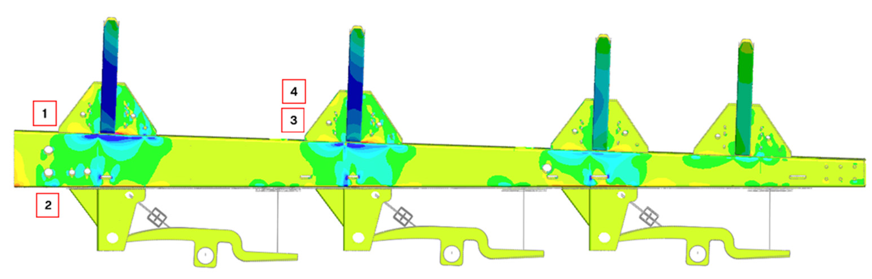
The turning load case involved the tank driving at 30mph while performing a slalom manoeuvre, turning from left to right. The results at all locations show a good correlation; however, the higher stress levels at locations 3 and 4 display more noise. Considering the surface we were driving on was very uneven and would induce much noise, the correlation is sufficient for us to regard the model as validated in the two main load cases of braking and turning.
Figure 15.
Braking Y Stress contour plot of the Tank Chassis.
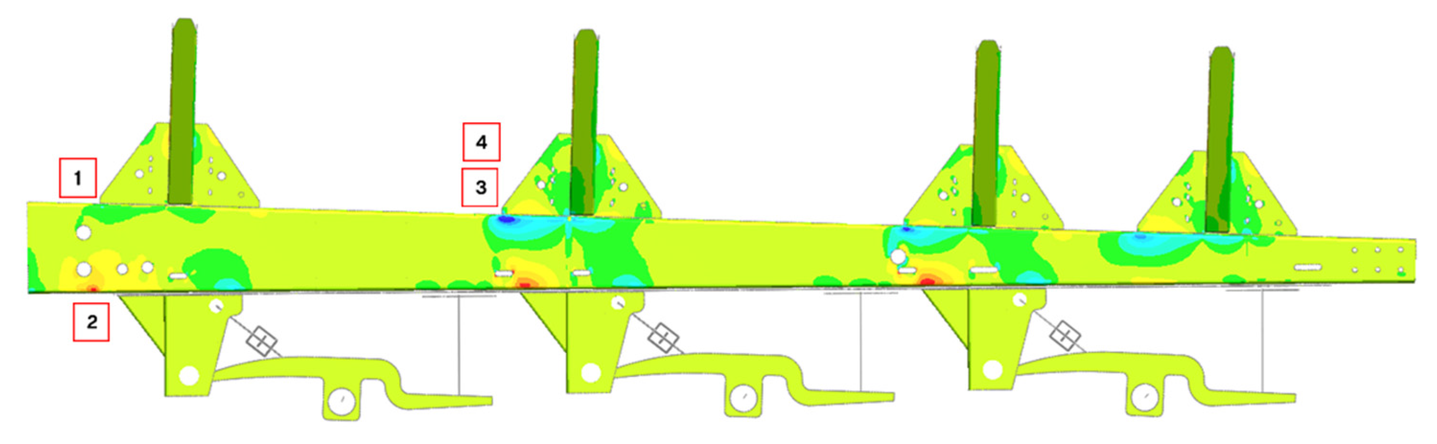
Figure 16.
Turning stress comparison of FEA results to Strain Gauge.
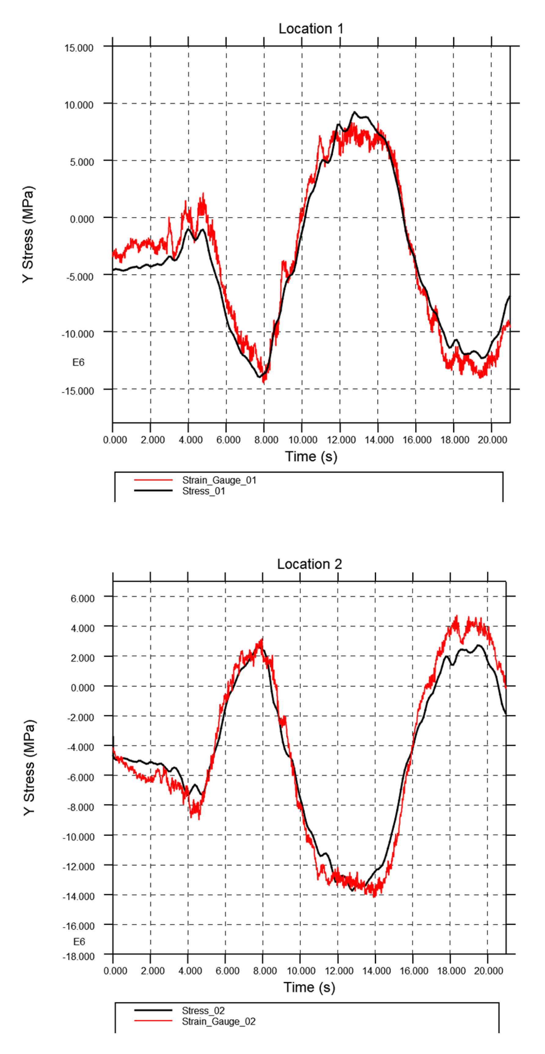
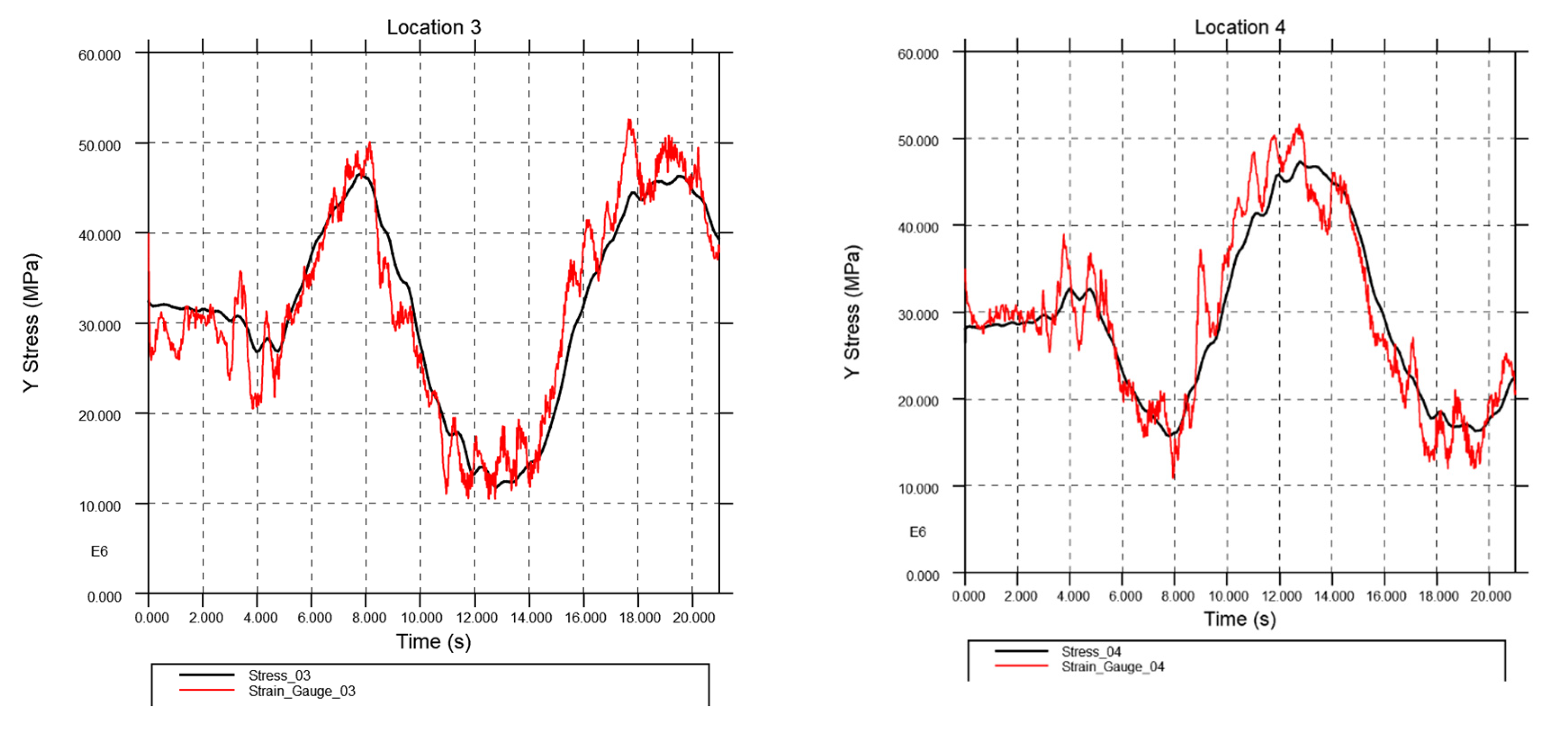
Figure 17.
Turning Y Stress contour plot of the Tank Chassis.
5. Multiphysics Tanker Model Results
Satisfied that the model had been validated, we felt confident in the results that we were seeing for the full tanker model. This enabled us to identify three primary areas for future development.
5.1. Hangers and Chassis
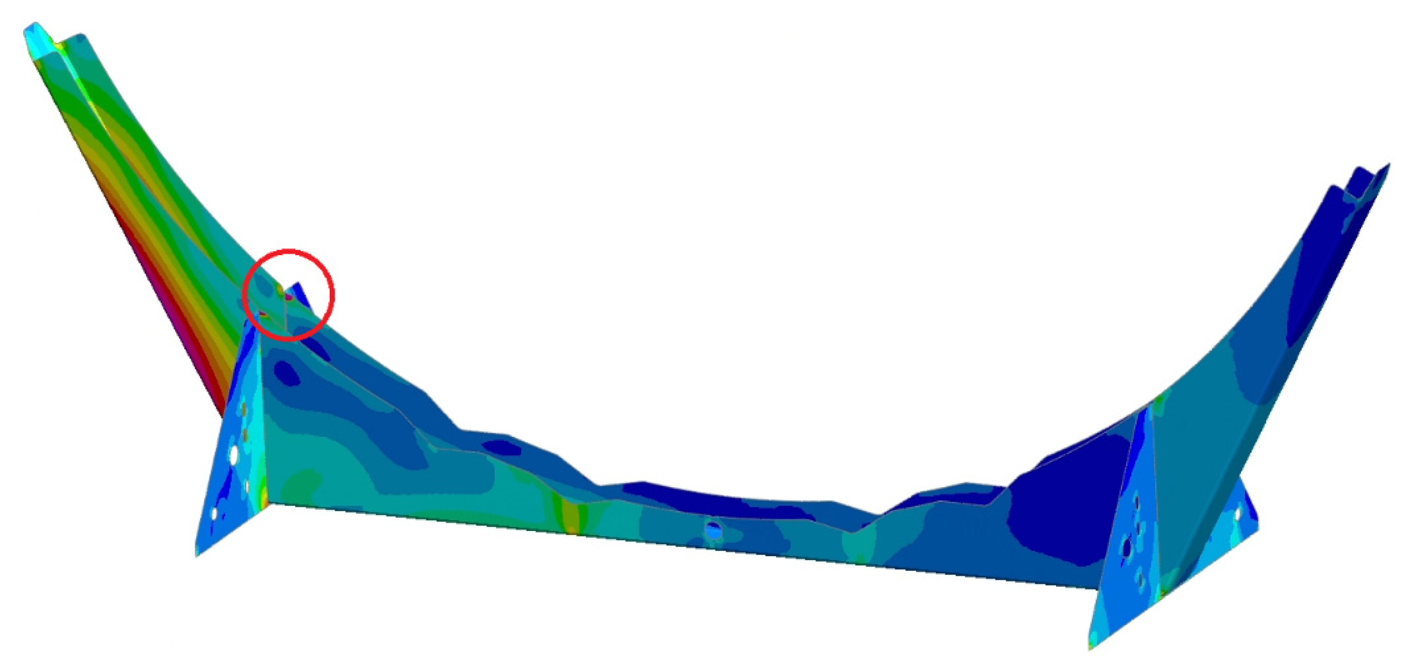
Figure 18 shows more of the stress bands throughout the structure. We can see that the front ring, bearer and hanger take the largest load. This confirms what Crossland engineers already believed to be true.
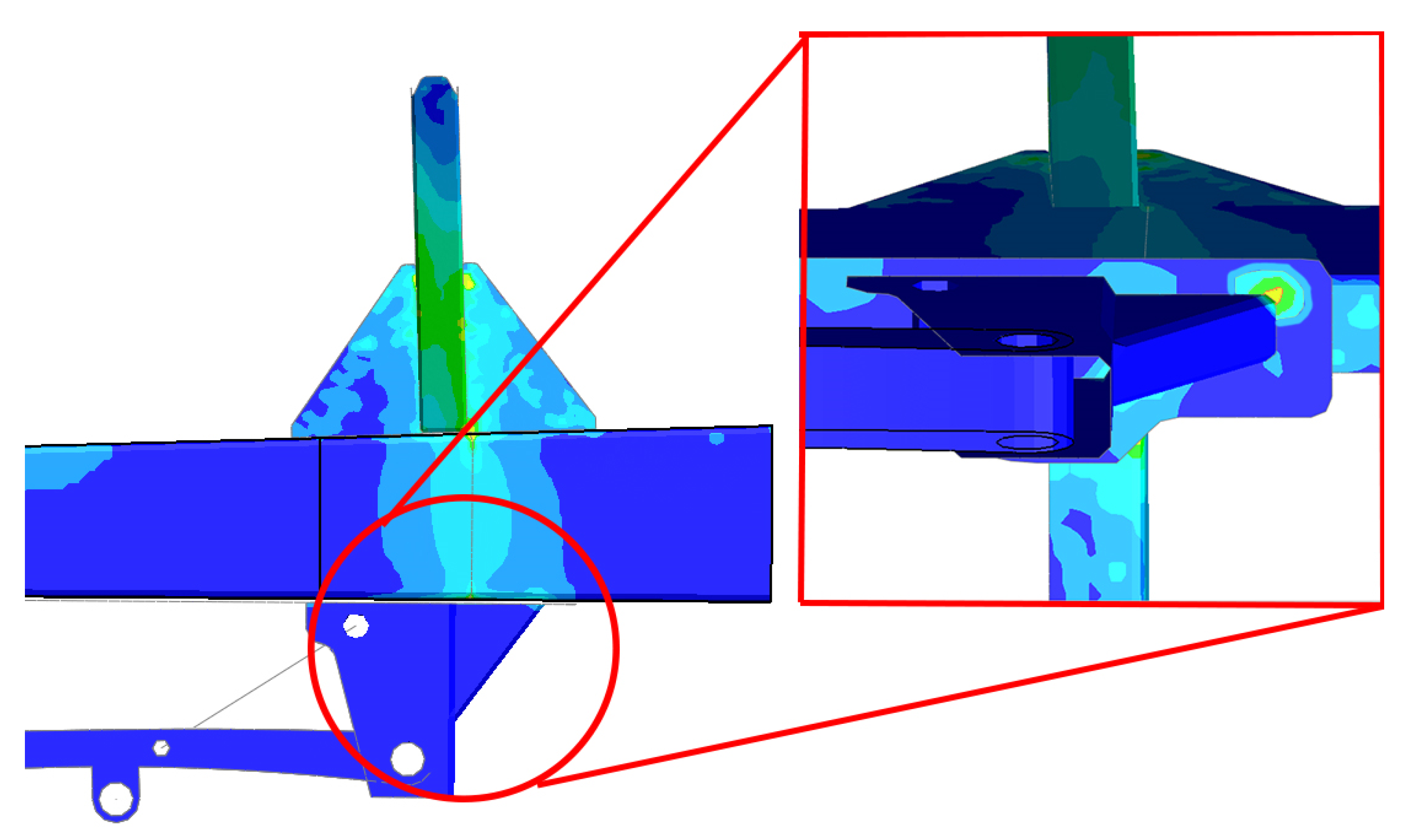
The hangar serves as a significant bracket connection point for the suspension arm and damper, as shown in Figure 19. The area where it joins the bottom of the chassis experiences cyclical stress with every brake, as indicated in the FEA results.
This area is also significantly influenced by road conditions, which are not factored into this model due to the absence of acceleration data from the axles. In future work, this data can be integrated to account for road vibrations and may reveal additional stress concentrations at the junction where the chassis and hangar meet.
5.2. Bearers
The bearers are the structure that connects the rings of the tank to the cassis, and as such, they experience significant stresses, especially under turning, when they are loaded unsymmetrically. Figure 19 shows the stresses on one arm.
Figure 19.
Von Mises stress plot for bearer under turning.
In this area, the three components move in different directions, creating a concentration of forces at the seam weld. One potential improvement is to merge the two parallel parts into a single component, removing the need for a weld and simplifying the design. The bearer typically performs well during braking, as the load remains balanced on both sides of the arm.
6. Conclusion
6.1. Summary of Key Findings
From our Multiphysics Road Tanker model, it was determined that the tanker under full load (gross vehicle weight, GVW) is the worst-case scenario and should be used as the load case for tanker design. Dynamic loads caused by sloshing significantly impact driveability and generate shock loads to the tank; however, the full weight of a fully loaded vehicle creates a higher peak stress on the chassis and components during braking and turning. SPH sloshing simulations are an important part of the design process and have numerous applications for baffle and rollover safety; however, sloshing is negligible at the Gross Vehicle Weight (GVW). This means that during the initial design phases, the SPH can be substituted for cheaper solid elements to speed up the simulation time.
Using real-world data collected from accelerometers and strain gauges, we were able to validate the FEA model with good accuracy and have confidence in integrating FEA into the design process at Crossland.
We have identified three areas that could be optimised as part of a weight reduction redesign for the chassis. The knowledge base at Crossland was strengthened through the use of clear explanations and visualisations that support ongoing engineering development. FEA results highlight areas of loading, particularly where multiple components are joined by welds.
To optimise these regions, future designs will aim to consolidate parts into single components where feasible, reducing the need for welding. This approach also offers benefits such as simplified manufacturing and reduced reliance on highly specialised welding techniques
6.2. Implications for the Design and Manufacturing of Road Tankers
The integration of a Multiphysics model, as described in this paper, should be incorporated into the design process at Crossland. Digital prototyping offers numerous advantages, enabling more ambitious designs to be pursued without the financial burden associated with physical prototyping. Individual parts can be refined and updated on the road tanker to assess their effectiveness in worst-case scenarios. Now that the process of creating this road tanker model is understood and effective automation techniques are established, a model can be developed relatively quickly for different tanker variants.
Our Material model of S304 has been validated using tensile load tests, allowing us to perform FEA compliance tests for components, such as crash bars, instead of costly physical tests.
6.3. Recommendations for Future Research and Development
Now that the strengths and weaknesses of the current design are understood, a new chassis should be digitally prototyped and validated in a similar manner. This will drastically reduce the development time for Crossland and improve the success rate of the prototype.
Fatigue testing will also be conducted and integrated into the S304 material model. This further expands the options for types of analysis on the tank and new components.
Road vibrations can be used in an NVH analysis in conjunction with fatigue data to evaluate the lifespan of the design over a range of different road conditions, depending on the region in which the tank is designed to operate.
References
- Otremba, F., Romero Navarrete, J. A., & Lozano Guzmán, A. A. (2018). Modelling of a Partially Loaded Road Tanker during a Braking-in-a-Turn Manoeuvre. Federal Institute for Materials Research and Testing (BAM), Berlin, Germany. Instituto Politécnico Nacional, CICATA-Querétaro, Querétaro, Mexico; Accepted 1 August 2018; Published 1 August 2018.
- Zheng, X.-l., Li, X.-s., Ren, Y.-y., Wang, Y.-n., & Ma, J. (2013). Effects of Transverse Baffle Design on Reducing Liquid Sloshing in Partially Filled Tank Vehicles. College of Traffic, Jilin University, Changchun, China. Received 17 July 2013; Revised 12 October 2013; Accepted 20 October 2013.
- Xu, J. , Wang, J., & Souli, M. SPH and ALE formulations for sloshing tank analysis. LSTC, Livermore Software Technology Corp., Livermore, CA, USA. Université de Lille Laboratoire de Mécanique de Lille, UMR CNRS 8107, France.
- Delorme, L.; Colagrossi, A.; Souto-Iglesias, A.; Zamora-Rodrigues, R.; Botia-Vera, E. A set of canonical problems in sloshing, Part I: Pressure field in forced roll-comparison between experimental results and SPH. Ocean Eng. 2009, 36, 168–178. [Google Scholar] [CrossRef]
- Landrini, M.; Colagrossi, A.; Faltinsen, O.M. Sloshing in 2-D flows by the SPH method. In Proceedings of the 8th numerical ship hydrodynamics, Busan, Korea, 22–25 September 2003. [Google Scholar]
- Chen, Z.; Zong, Z. ; Li, HT; Li, J. An investigation into the pressure on solid walls in 2D sloshing using SPH method. Ocean Eng. 2013, 59, 129–141. [Google Scholar]
- Jonsson, P. , Jonsén, P., Andreasson, P., Lundström, T.S., & Hellström, J.G.I. Modelling Dam Break Evolution Over a Wet Bed with Smoothed Particle Hydrodynamics: A Parameter Study. Division of Fluid and Experimental Mechanics, Luleå University of Technology (LTU).
- Kweon, H. D. , Kim, J. W., Song, O., & Oh, D. Determination of true stress-strain curve of type 304 and 316 stainless steels using a typical tensile test and finite element analysis. Korea Hydro & Nuclear Power Co, Ltd., 70, 1312-beongil, Yuseong-daero, Yuseong-gu, Daejeon, 34101, Republic of Korea.
- Kweon, H. D. , Heo, E. J., Lee, D. H., & Kim, J. W. (2018). A methodology for determining the true stress-strain curve of SA-508 low alloy steel from a tensile test with finite element analysis. Central Research Institute, Korea Hydro and Nuclear Power Co., Daejeon, Korea.
- Romero, J. A. , Otremba, F., & Lozano Guzmán, A. A. Simulation of liquid cargo–vehicle interaction under lateral and longitudinal accelerations. Faculty of Engineering, Queretaro Autonomous University, Mexico.
Figure 1.
Multiphysics Tanker Model.
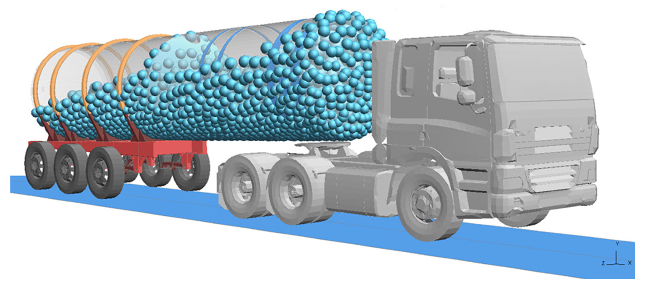
Figure 2.
Tank Fluid Slushing Simulation in LS-Dyna.
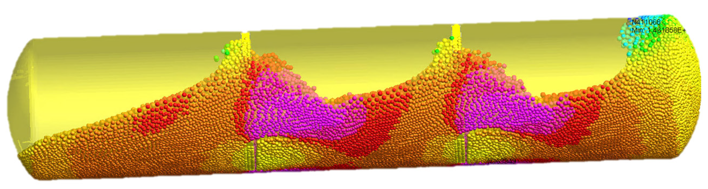
Figure 3.
Artificial Viscosity comparisons.
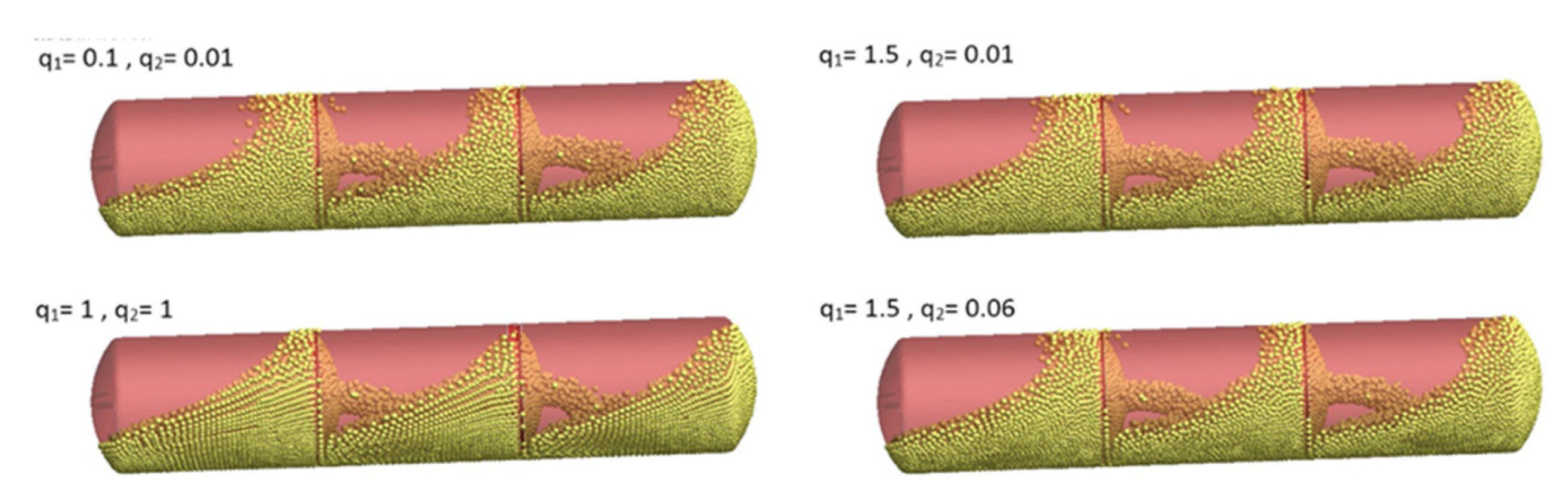
Figure 4.
SPH Parametric Study.
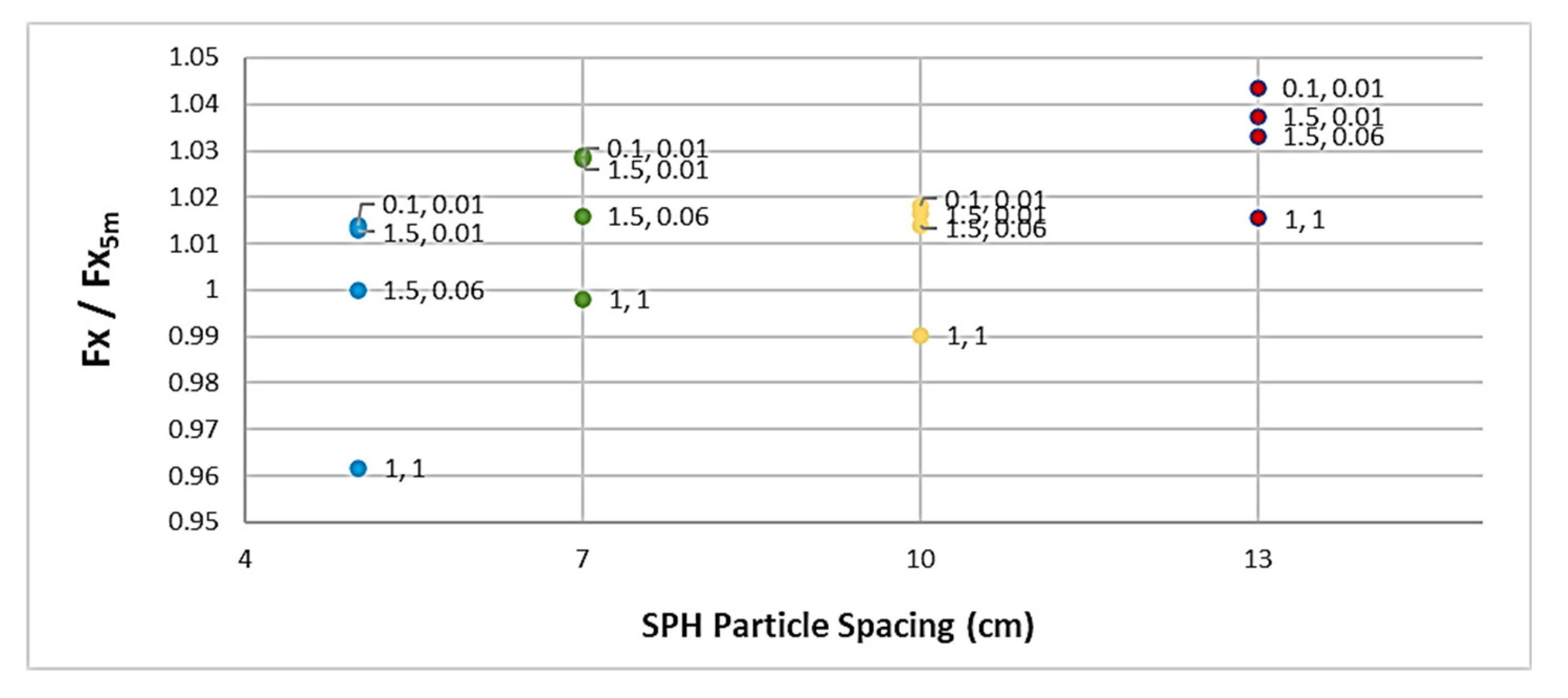
Figure 5.
Mid-Surface Extraction and Meshing of Components.
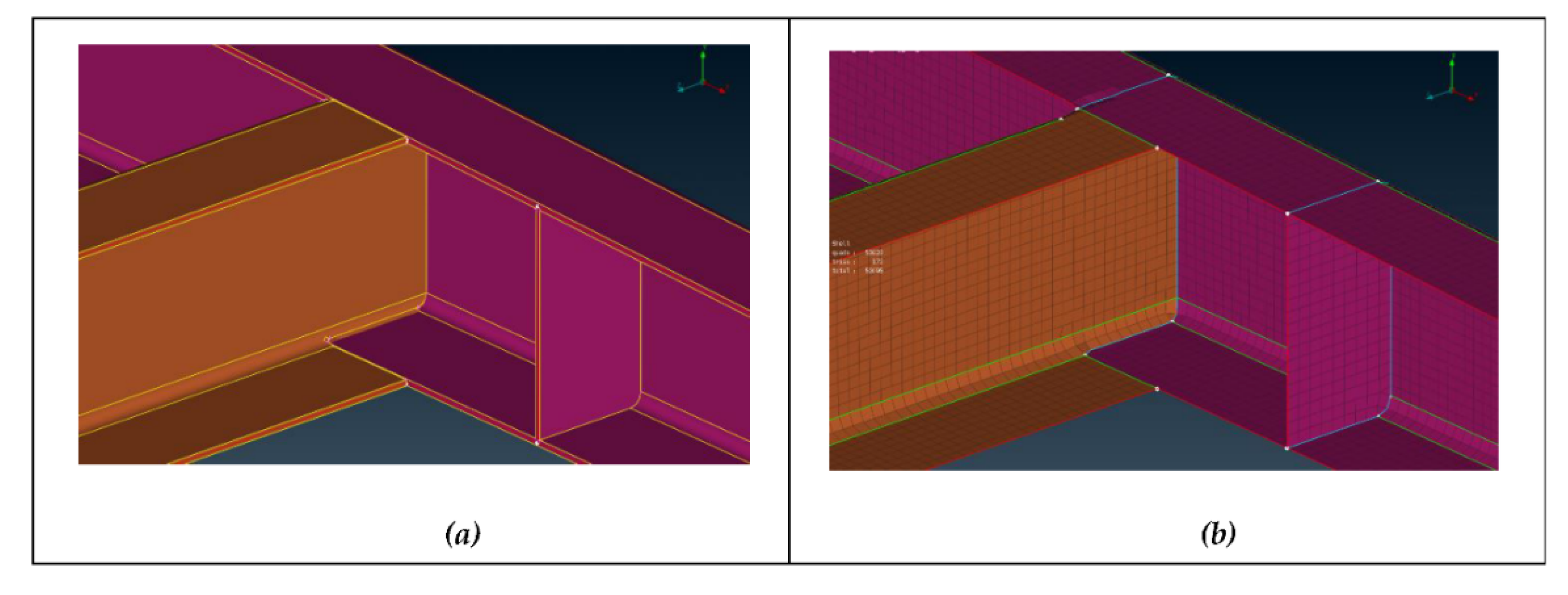
Figure 6.
Axle suspension and FEA model.
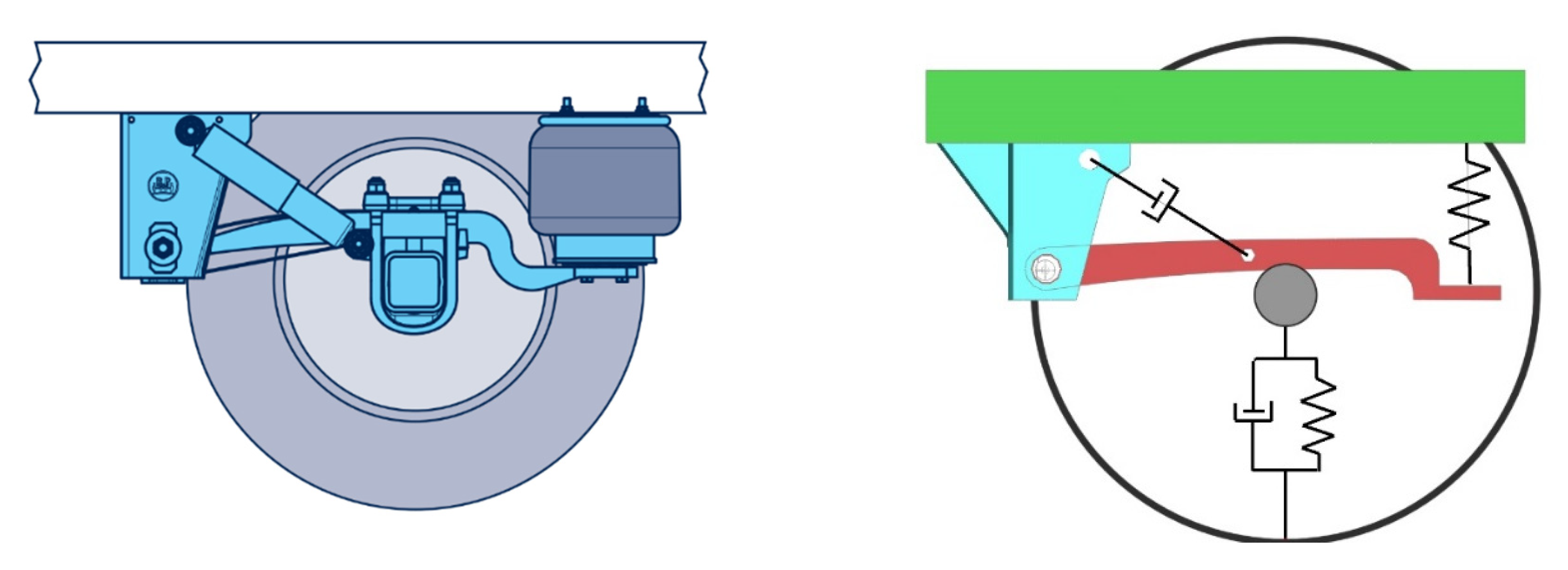
Figure 7.
Engineering Stress-Strain curves of test samples and average.
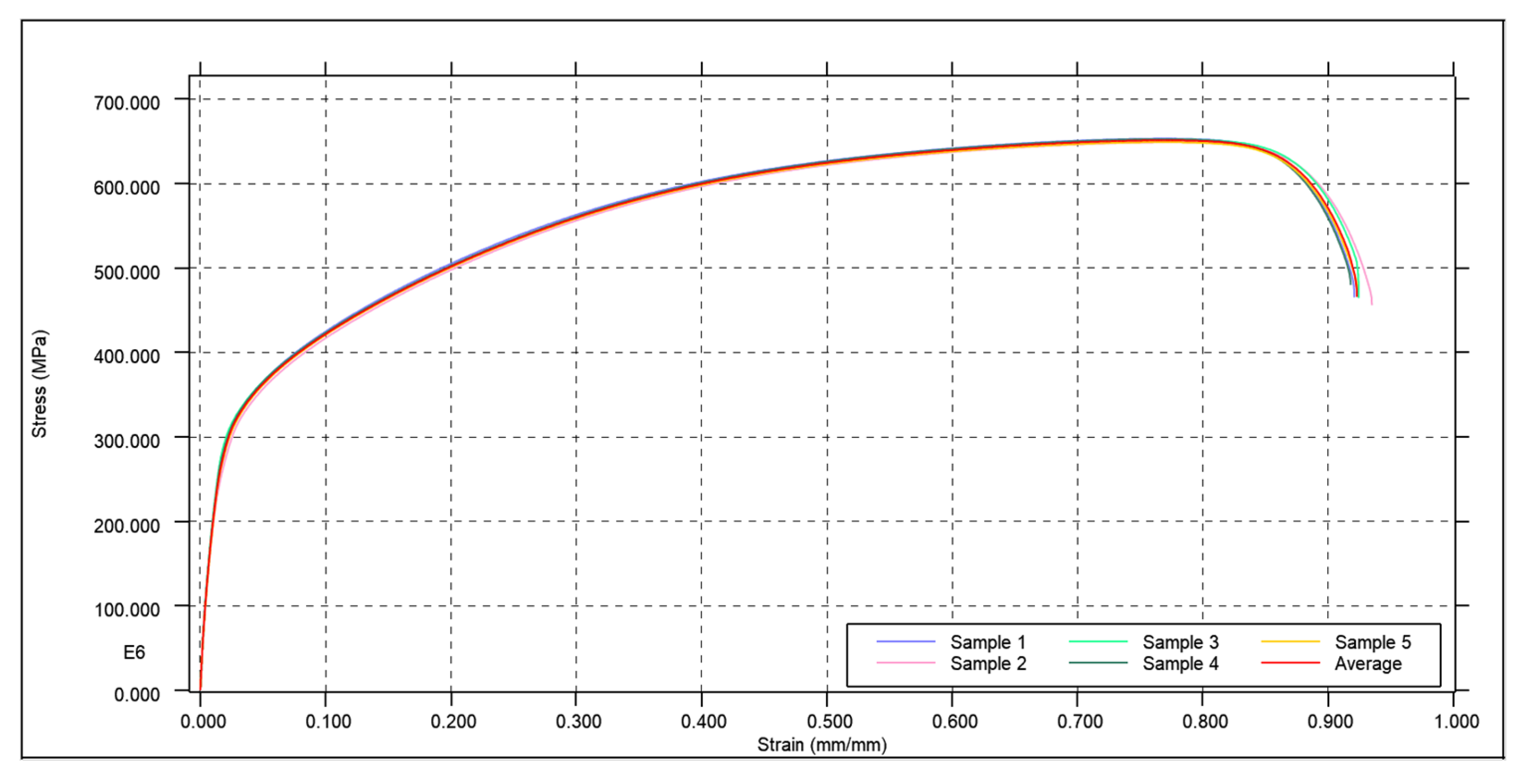
Figure 8.
Corrected true Stress-Strain curves and FEA results.
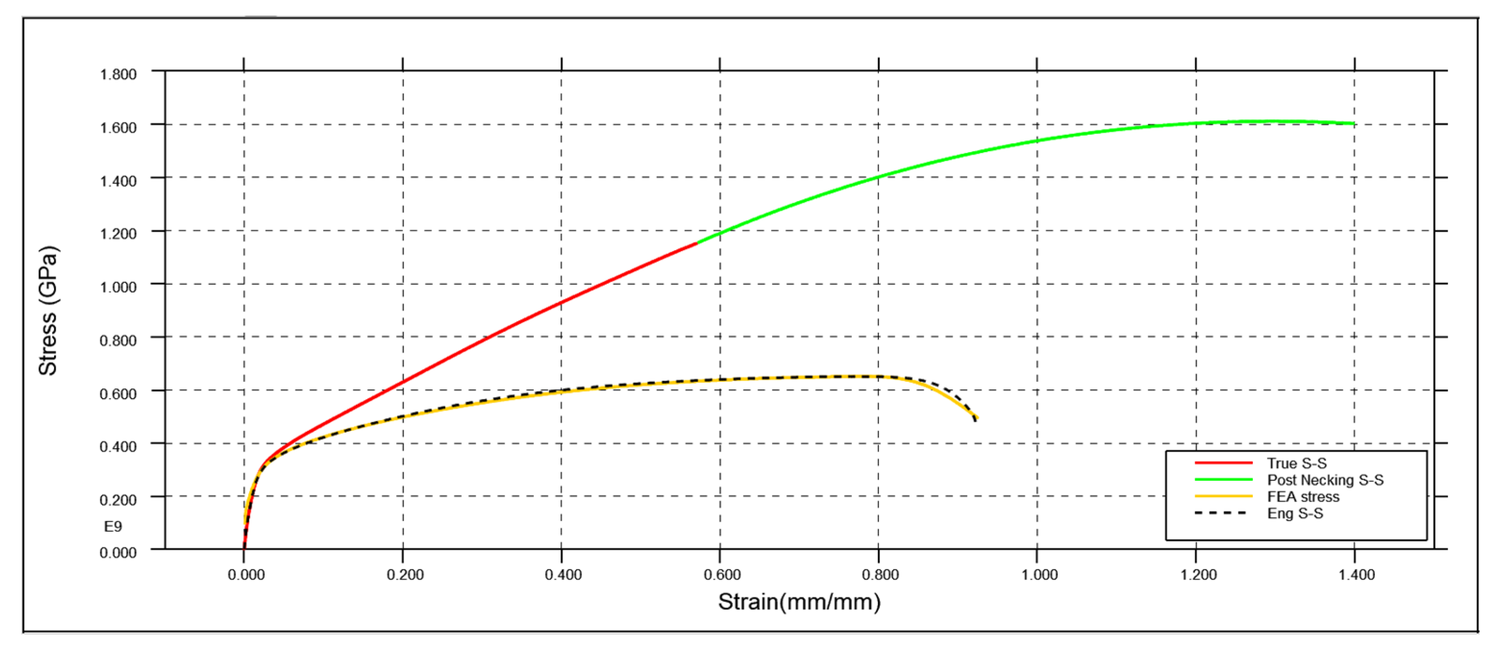
Figure 9.
FEA tensile quarter model.
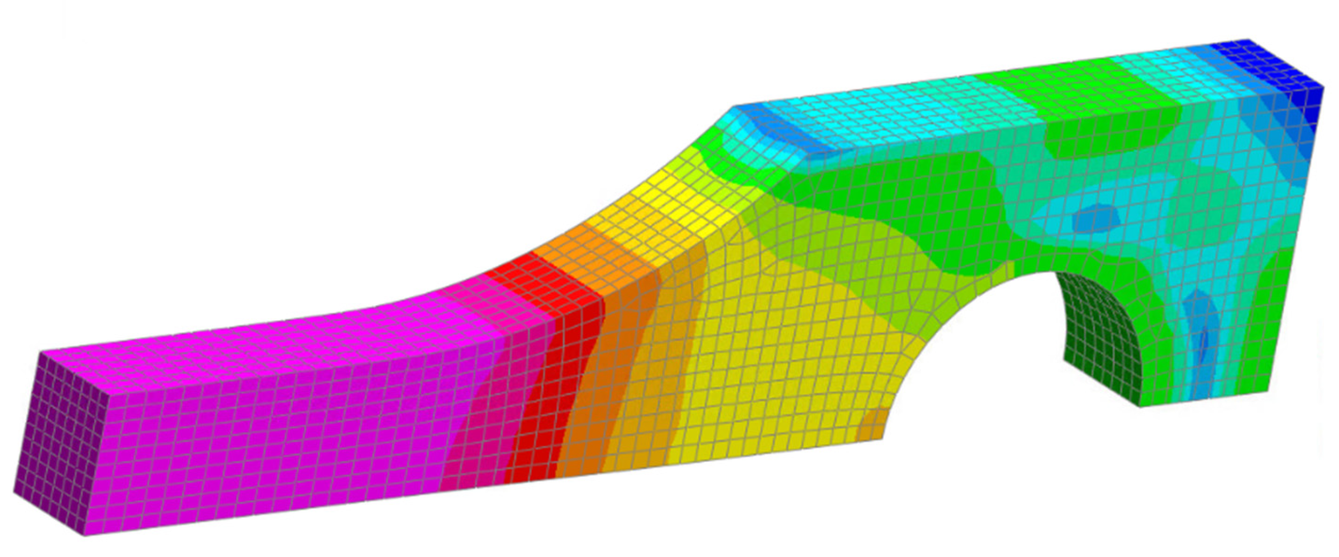
Figure 10.
Accelerometers and strain sensor locations.
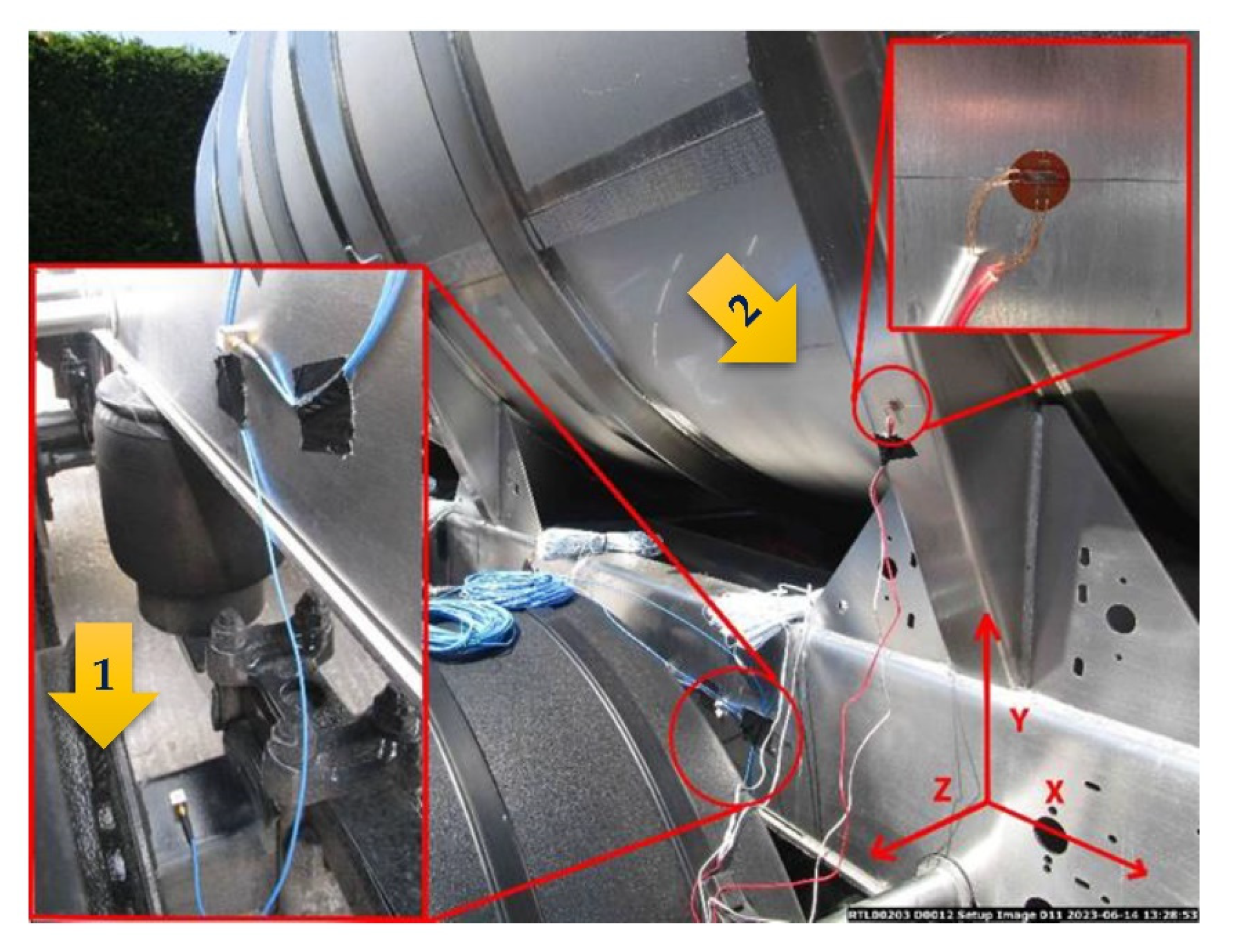
Figure 11.
Acceleration and velocity data from Test 1.
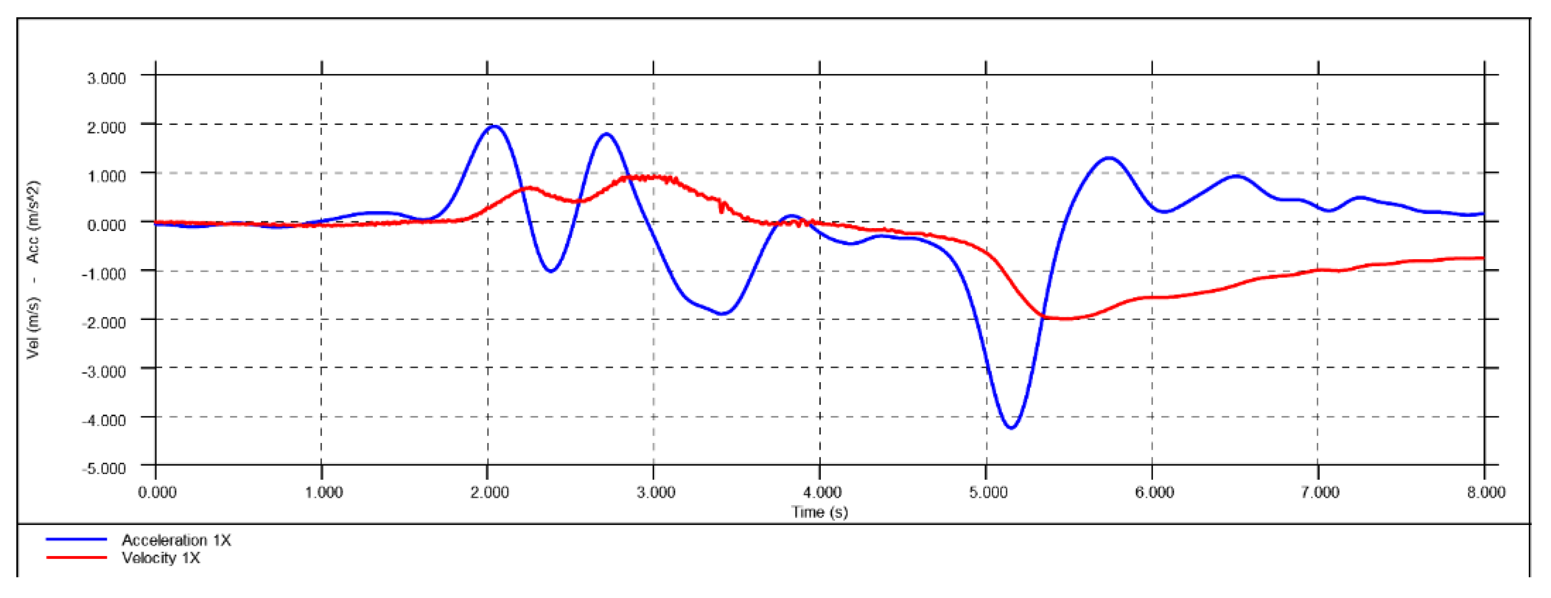
Figure 12.
Real-world acceleration and velocity data from phone accelerometers.
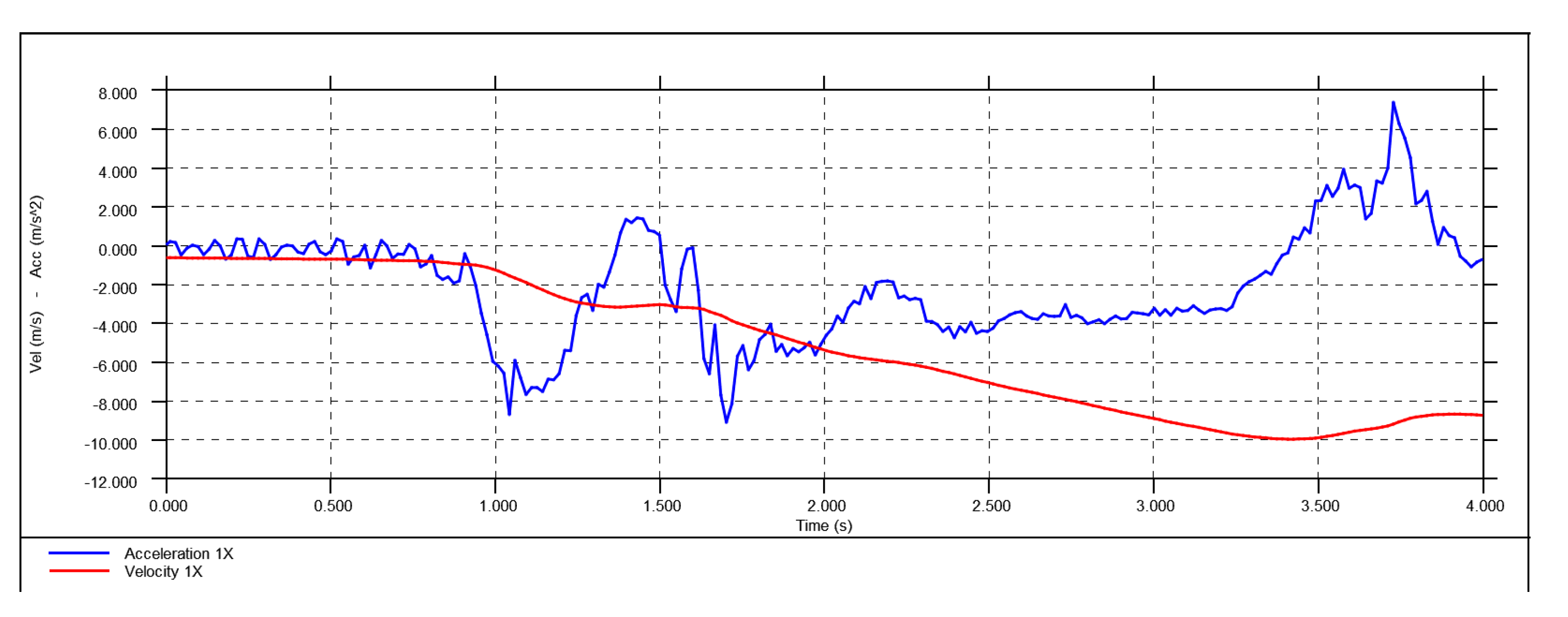
Figure 13.
Test 2 Acceleration and Velocity from MEMS.
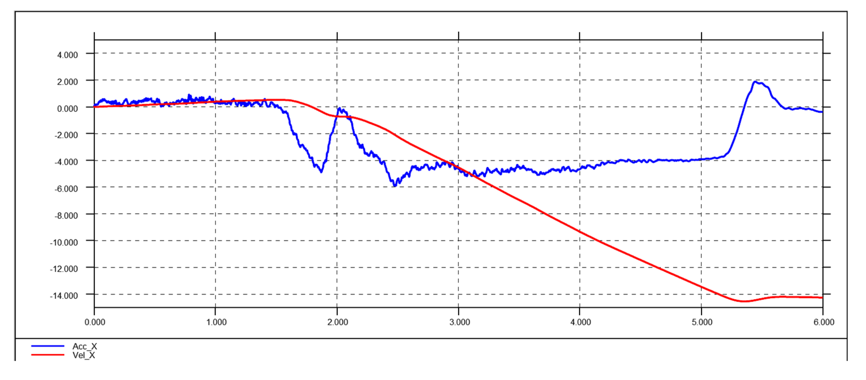
Figure 14.
Braking stress comparison of FEA results to Strain Gauge.
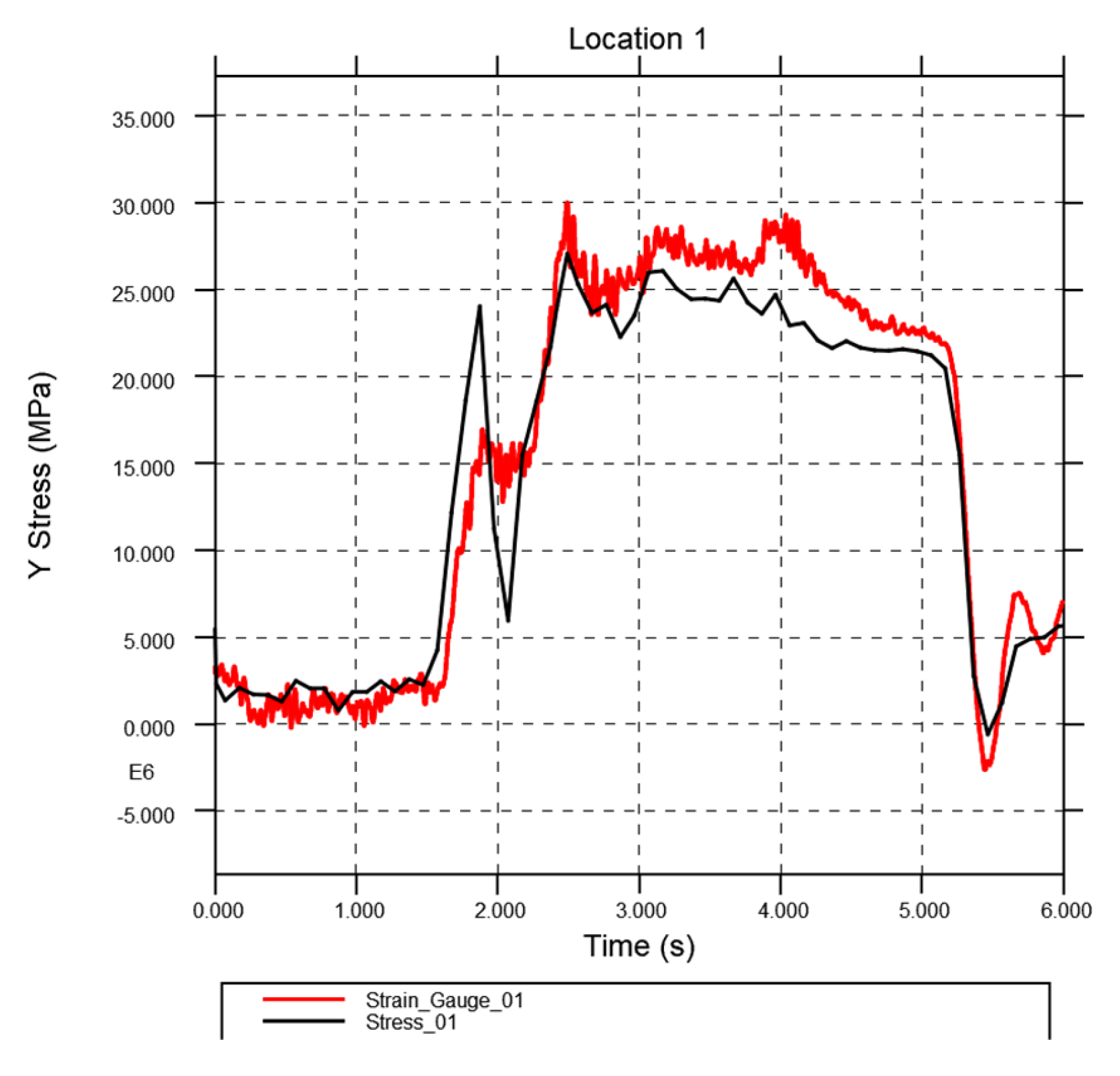
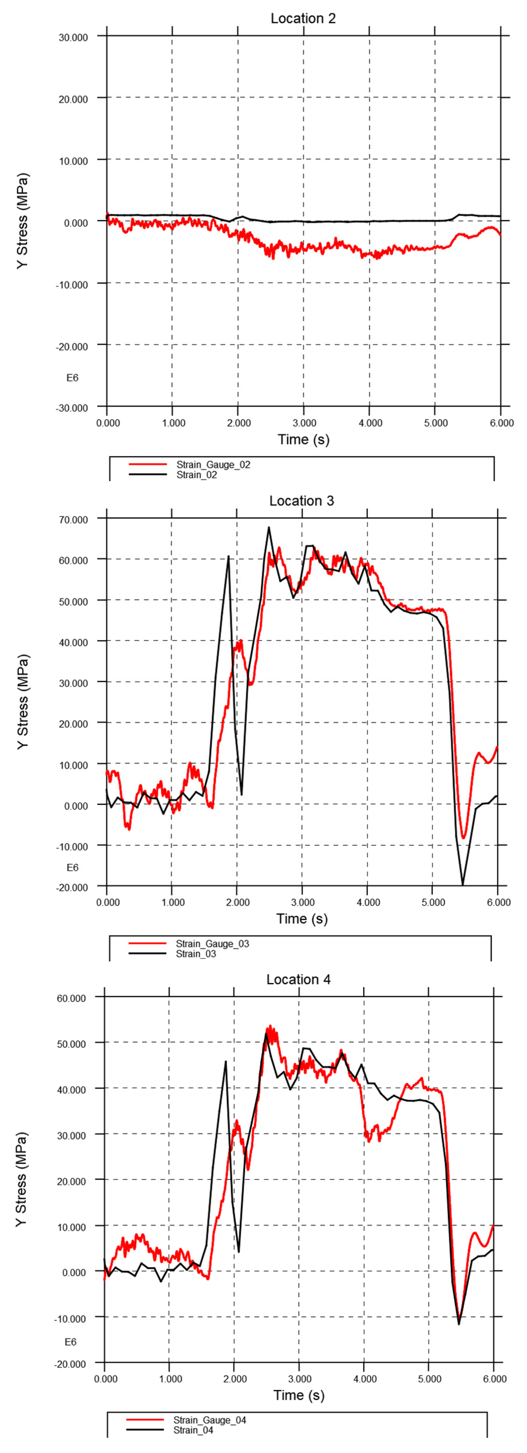
Figure 18.
Von Mises stress plot for the tanker under braking.
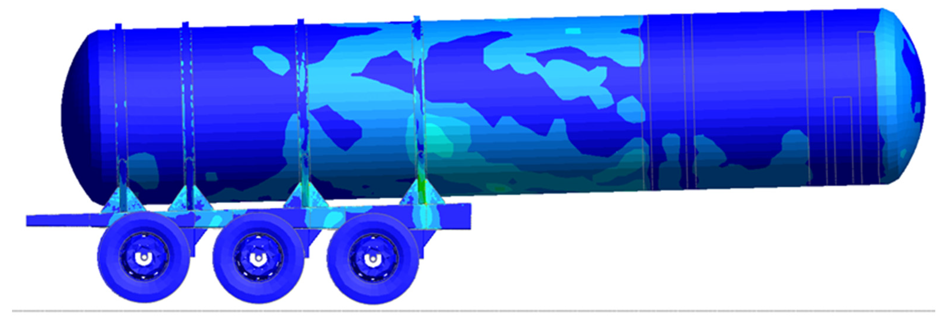
Figure 19.
Closeup of chassis and hangar.
Disclaimer/Publisher’s Note: The statements, opinions and data contained in all publications are solely those of the individual author(s) and contributor(s) and not of MDPI and/or the editor(s). MDPI and/or the editor(s) disclaim responsibility for any injury to people or property resulting from any ideas, methods, instructions or products referred to in the content. |
© 2025 by the authors. Licensee MDPI, Basel, Switzerland. This article is an open access article distributed under the terms and conditions of the Creative Commons Attribution (CC BY) license (http://creativecommons.org/licenses/by/4.0/).
Copyright: This open access article is published under a Creative Commons CC BY 4.0 license, which permit the free download, distribution, and reuse, provided that the author and preprint are cited in any reuse.


