
Submitted:
29 May 2025
Posted:
30 May 2025
You are already at the latest version
Abstract
This study employs a bespoke Machine Learning infrastructure to unravel the complex dynamics of e-waste supply chain networks (SCNs) by optimizing a Euler-Lagrange cost function. The framework analyzes the interconnections of the concerned variables (and parameters) with the three pillars of sustainability, eventually ranking their relative contributions towards the optimization of the SCNs. To analyze the resilience of the economic SCN and its ability to converge to optimality when perturbed by external factors, using data from an Indian e-waste plant, we use Monte Carlo simulation to generate four stochastically perturbed modules around the optimal point of the original dataset. To identify the emerging nonlinear patterns, a Neural Network (NN) model has been combined with a Random Forest Model (RFM) for ensemble-based feature selection. Our results consistently point to NN as a better predictor of arbitrage conditions compared to RFM. The juxtaposition of these two models reveals a trade-off between predictive power and interpretability. While the NN serves as a potent tool for uncovering hidden complexity and emergent behaviors, the RFN proves invaluable for feature engineering, scenario simplification, and system pruning. Together, they outline an optimized toolbox that ensures sustainable production through smart engineering solutions.
Keywords:
supply chain network (SCN)
; machine learning (ML)
; Monte Carlo (MC) simulation
; neural network (NN)
; random forest model (RFM)
1. Introduction
The last decade has witnessed an overwhelming surge in electronic waste, popularly called e-waste, generation due to high rates of product desuetude (Kavil et al. 2025). The combination of digital dependency and digital necessity in a modern world has driven complex sustainability challenges (Campana et al. 2025). As the fastest growing urban waste stream, e-waste poses high environmental risk but also presents an untapped opportunity of repurposing secondary raw materials (Choi et al. 2023). Resilient supply chain systems are key to responsible resource recovery from secondary materials, reducing environmental impact and in highlighting circular economy which directly aligns with SDG 12 (Responsible Consumption and Production) and SDG 11 (Sustainable Cities and Communities) (Bhatnagar and Dixit 2025).
Traditional supply chain models often rely on equilibrium optimization techniques that focus only on static equilibrium properties and hence are inadequate in capturing the time-sensitive, nonlinear, and feedback-driven behavior typical of real-world systems. To address this limitation, Debnath, et al. (2022) developed a novel supply chain network analysis framework, pioneering an altogether different modelling approach, drawn from the lexicon of classical mechanics, that treats supply chain logistics analogous to chemical reaction kinetics where the key features are seen an evolutionary, that is time dependent, rather than time-morphed with an unchangeable (and hence unphysical) arbitrage point. The mathematical infrastructure was based on the established Euler-Lagrange formalism (Goldstein, et al. 2011) which led to a paradigm shift enabling the dynamic mapping of material, information, and value flows across supply chain nodes, analyzing the temporal evolution and systemic feedback loops.
Building on this foundational framework, a subsequent study by (Debnath, et al. 2024) optimized an e-waste Supply Chain Network (SCN) using machine learning tools. This model successfully explained system-wide (i.e. dynamic) equilibrium behavior and supported sustainable production planning by aligning economic efficiency against environmental objectives (Leong et al. 2025). However, a critical question remained unexplored: Do the observed dynamical states define stable equilibria, or do they represent saddle point zones, that is, regions of metastability that can be easily perturbed towards an unstable conformation? This understanding will be key to business and environmental sustainability.
The present study addresses this knowledge gap by stochastically perturbing the original kinetic model (Debnath et al. 2022) within a Monte Carlo framework (Mun 2015) and then studying whether the perturbed equilibrium can eventually converge to its previously predicted (deterministic) equilibrium state (Gao et al. 2022). To analyze, we simulate 4 datasets (1 key data set and 3 perturbed data sets) for each variable from the original model, identify “irrelevant” parameters (i.e. parameters which do not cause any major fluctuation in the supply chain performance), and then perturb only the relevant parameters using Monte Carlo simulations to ascertain system robustness (Bruni Prenestino et al. 2025). The incorporation of controlled randomness enables us to test the sensitivity and structural resilience of the modeled e-waste supply chain, examining whether the system returns to equilibrium or transitions away along unstable saddle trajectories (Singh et al. 2025).
To analyze the complexity of the emergent system and pinpoint the latent drivers of instability, we deploy a state-of-the-art deep learning (Neural Network) and a machine learning (Random Forest) tool: (a) a Neural Network (NN), capable of capturing non-linear dependencies in addition to features (Kalbunde et al. 2025), and (b) a Random Forest Network (RFN) (Imani et al. 2025), which excels at ranking feature importance via ensemble learning.
This article targets three key objectives:
- Explore whether the stochastically perturbed kinetic system converges to a stable equilibrium or exhibits metastable saddle behavior under stochastic perturbations. Convergence to a stable equilibrium will point to a resilient economic SCN while a saddle point will point to probabilistically unreliable SCNs.
- Extract embedded and latent features using established Machine and Deep Learning algorithms (Deep Neural Network and Random Forest). This will identify the key variables within the e-waste supply chain network from a much wider set of potential contributors. The eventual minimalist model will use these key variables only.
- Generate and analyze four alternative scenarios beyond the base case (original dataset). This will allow us to design and predict parametric spaces within which the system will converge to a resilient SCN (point 1 above).
Such Artificial Intelligence (AI) driven predictions on supply chains, analyzing dynamic, real-world scenarios, are expected to pave the way for a resilient, adaptive, and intelligent e-waste management systems (Nweje and Taiwo 2025).
2. Methodology
2.1. Baseline Model
The base structure of this study is contemplated in the framework developed by (Debnath et al., 2022), where SCNs are modeled as interconnected dynamic reaction networks analogous to chemical systems. The model utilizes a cost function that encompasses all key nodes of a supply chain based on three verticals of sustainability, including uncertainty. Time evolving performance of this SCN, modeled as a Euler-Lagrange framework, is then undertaken to identify key players, and then extract a minimalist model from the starting generalized framework as in the original study (Debnath, et al. 2022; Debnath, et al. 2024).
This study is structured on three key remits:
- Introduction of stochasticity via Monte Carlo perturbations in quasi-static variables.
- Application of Machine Learning (ML) to assess the sensitivity and relevance of individual features.
- Exploring multiple simulation scenarios to test the robustness of the originally observed equilibria.
By revisiting the baseline model through a lens of stochastic resilience and feature-driven complexity analysis, this study aims to both challenge and refine the conclusions drawn from the original kinetic modeling effort.
2.2. Dataset Management
Initially, anonymous SCN performance data of a month was collected from a multi-award-winning Indian e-waste company (details cannot be disclosed due to IP rights). To ensure unambiguous data with minimized outliers, we engaged in phased discussions with the company. These discussions enabled us to identify key variables from the industrial perspectives. To analyze whether these experience-based assertions match with data modeled deductions, we gathered data for another 1.5 years. Overall, considering each month’s data as a singular entry we recorded 18 entries, translating into a 24 x 18 data matrix. Missing data were cloned from previous trend lines and the authors’ experience. This comprised the core dataset for the benchmark case.
2.3. Variable Behavior Analysis
Starting from all possible contributors to the e-waste SCN, after consultation with the industry, many of these were later retracted as “irrelevant” or “redundant” variables for the industry in question, an input based on real-life experiences of the industrial exponents. Once the core set of potential variables (and parameters) were identified, we extracted three stochastically perturbed datasets starting from the original dataset using Monte-Carlo Simulations (MCS). Addressing the stability aspect of the emergent model and risk validation through MCS is the key novelty of this study. If the perturbed states converge to the stable fixed points of the original data set (Debnath, et al. 2022; Debnath, et al. 2024), the SCN is regarded as generically stable; if not, we analyze points of instability as functions of specific variables.
2.4. Monte Carlo Simulation (MCS)
Monte Carlo (MC) simulation is a powerful computational technique that is structured on random sampling to model the behavior of complex systems and estimate the probability of different outcomes. The idea relies on identifying an equilibrium system as a maximally chaotic system, a “high temperature” state in the physics parlance, where all concerned atoms and molecules get hyperactive. The probability of finding any such (hyperactive) particle is obtained by weighing the corresponding state with a probability function that is drawn from a Boltzmann distribution.
In supply chain modeling, MCS is widely used in quantifying and mitigating the inherent uncertainties that characterize modern global logistics networks. Instead of relying on single-point estimates, Monte Carlo simulations generate a vast number of potential scenarios by sampling from (Boltzmann) probability distributions for key variables, such as customer demand, supplier lead times, transportation delays, and even production yields. The highest temperature state is popularly identified as the steady state when the SCN performance is expected to bear a probabilistic connection to past statistical performance of the SCN. This is the premise on which we build.
2.4.1. Monte Carlo for e-waste SCN
We used Monte Carlo simulation to perturb the original multidimensional e-waste data from a spreadsheet to introduce stochastic perturbations, enabling the exploration of uncertainty and the generation of perturbed manifolds. This was done using a Visual Basic (VBA) code that we wrote for the purpose. The performance of the code is limited compared to specialized statistical software like SPSS or Strata, but its widespread, and more importantly, open-sourced access makes it a common starting point for data. By defining variable probability distributions (we used normal and uniform) for key input variables within Excel cells, Monte Carlo was implemented using simple VBA macros to repeatedly sample from these distributions. Each iteration generated a slightly varied dataset, effectively creating a “stochastically perturbed” version of the original.
This process is particularly useful when the data represents points on a manifold (a high-dimensional surface or structure) and one wishes to understand how noise or uncertainty in the input measurements propagates to the shape or features of that manifold. For our e-waste data that is often sparse or contains inherent measurement errors, perturbing the Excel-based input data through Monte Carlo can generate numerous slightly different manifolds. Analyzing this ensemble of perturbed manifolds allowed for the quantification of uncertainty in the manifold’s geometry, the robustness of features extracted from it, or the sensitivity of downstream analyses to input variability. Apart from providing a more comprehensive risk assessment and a deeper understanding of the system’s behavior under noisy conditions, we used MCS to validate our supply chain kinetic predictions. This is the second novelty of this study.
2.5. Machine Learning Framework
a. Neural Network (NN)
Neural Networks (NNs) are a class of artificial neural networks characterized by multiple hidden layers between the input and output layers, enabling them to learn intricate patterns and hierarchical representations from complex data (Aggarwal, 2018). Each neuron within these layers processes input signals by applying a weighted sum of its inputs, augmented by a bias term, which is then passed through a non-linear activation function. This layered architecture allows NNs to model highly complex, non-linear relationships that single-layer networks cannot (Wang et al. 2023). For a single neuron in a hidden layer, its output, , can be expressed as:
Here represents the activations from the kth neuron in the preceding layer (l−1), are the synaptic weights connecting the kth neuron in layer (l−1) to the jth neuron in layer l, is the bias term for the jth neuron in layer l, and denotes the nonlinear activation function (e.g., ReLU, sigmoid, tanh).
The “deep” aspect comes from stacking many such layers, where the output of one layer serves as the input to the next. The entire network’s feed-forward process involves sequentially computing activations from the input layer through all hidden layers to the output layer (Jin and Sun 2025). This is the key reason for our choice. With a complex networked system involving multidimensional variables and parameters comprising an e-waste SCN (Vogt 2025; de Carvalho Freitas et al. 2025), a NN is perhaps better placed to analyze the nuance and extract the hidden features of the system. During training, the network learnt optimal weights and biases by minimizing a loss function, typically through backpropagation and gradient descent, which adjusts these parameters to reduce the discrepancy between predicted and actual outputs (Fuji et al. 2018).
b. Random Forest Network (RFN)
The Random Forest (RF) was chosen as the only Machine Learning module to compare the NN predictions as it stands out for its inherent robustness, enhanced interpretability, and exceptional proficiency in discerning intricate, non-linear relationships within data (Vairagade et al. 2019). As an ensemble learning paradigm, RF operates by constructing a multitude of decision trees during its training phase. For a given input, the final prediction is derived by aggregating the individual predictions from each of these constituent trees, typically by averaging them (Breiman, 2001). This collective wisdom approach significantly mitigates the perennial problem of overfitting, which is particularly prevalent in high-dimensional datasets, thereby ensuring the model’s strong generalization capabilities (Farazi 2015). Furthermore, RF offers a reliable mechanism for assessing the importance of individual features, primarily through the permutation importance method. Mathematically, the prediction of an RF model for a given input xx can be expressed as:
where B is the number of trees defining the interacting nodes, and is the prediction of the bth tree. The variable importance score for a feature was calculated as
Here is the mean squared error of the bth tree, and is the MSE obtained from permuting . This method ensures the suitability of RF in identifying key economic players in the analysis of the kinetic SCN.
3. Results and Discussions
The collected data comprises a total of 21 variables of which 5 are dependent variables, each of which depend on 16 independent variables. These are specific to the system and are not generic. The dependent variables are Volume of CO2 generated (VCO2); Energy Consumed (Ec), Water Consumed (Wp), Waste water Produced (Ww) and number of awareness activities and marketing per year (N3). The independent variables are as follows: Number of labors (N1), number of recycled materials (N4), number of operations (N5), number of logistics (N7), number of waste materials going to TSDF (N8), number of tax units (N9), unit cost of CO2 recovery (F1), unit cost of energy used (F2), unit cost of water used (F3), unit cost of wastewater treatment (F4), salary of one labor (F5), average cost of awareness activity & marketing (F6), unit revenue earned from recycled product sold (F7), unit cost of each operation (F8), unit cost of logistics (F10) and unit cost of disposal in TSDF (F11) are the independent variables. We have used two major ML algorithms, NN and RF for our analysis. We present one Benchmark Case and two perturbed cases in this study. For each case study, the first four figures are obtained from NN, and the last two figures are obtained from RF.
3.1. Case 1: Benchmark Dataset
Figure 2 represents the correlation between dependent and independent variables of the e-waste supply chain system. Independent variables 7 (F1), 9 (F3), 10 (F4), 12 -16 (F6 – F8, F10 and F11) are highly sensitive having most of the complex effects to the dependent variables except no. 5 which is N3. This means that the interaction between these variables are highest, contributing to high system entropy. On the other hand, independent variables 1-6 (N1, N4, N5, N7-N9), 8 (F2) and 12 (F6) are least affected.
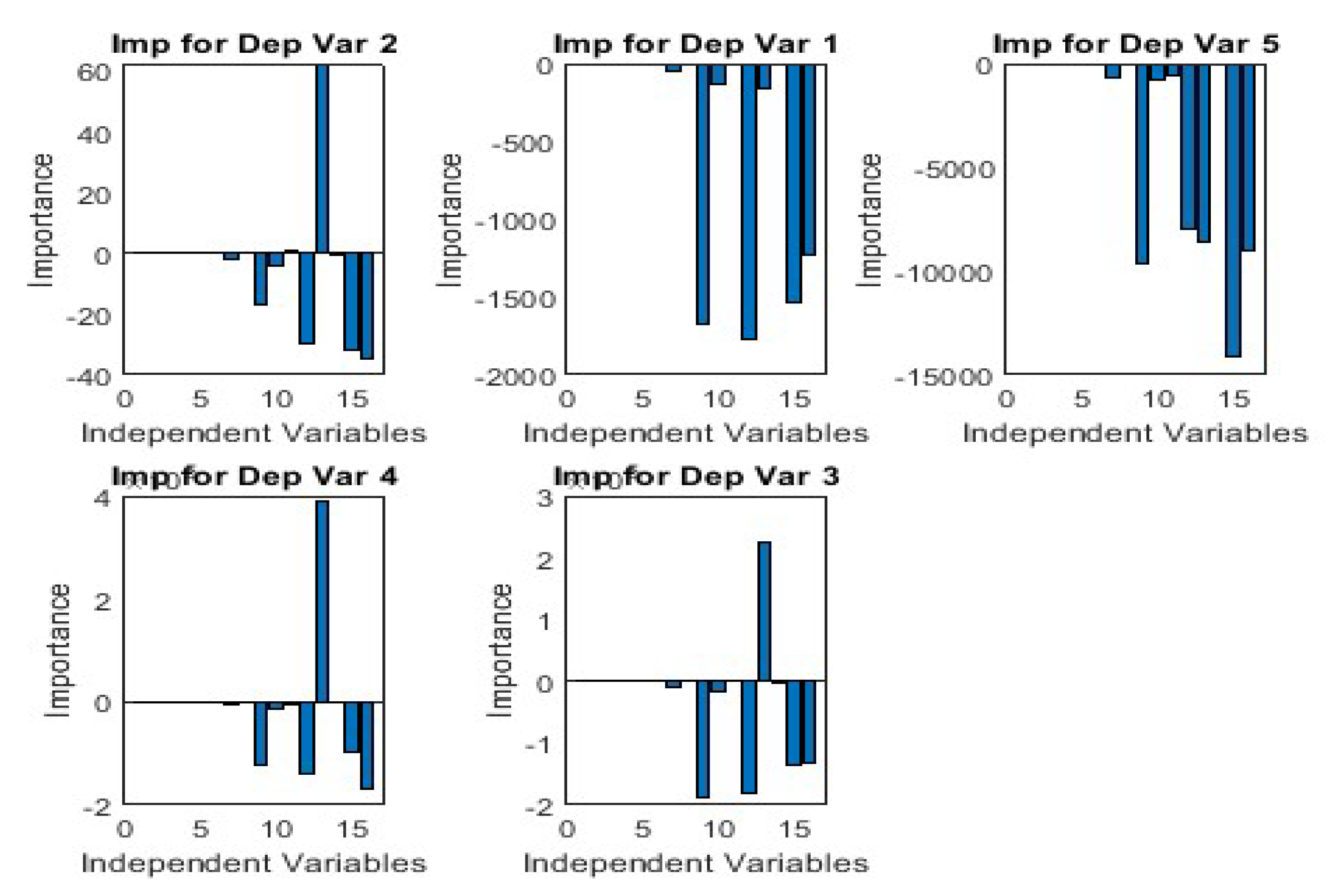
NN evaluation identifies the top 4 dependent variables are VCO2, Ec, Ww and Wp (Figure 2 and Figure 3). Further analysis of Figure 3 suggests the same. Although the overall importance direction is negative, the magnitude confirms to the initial analysis of Figure 2.
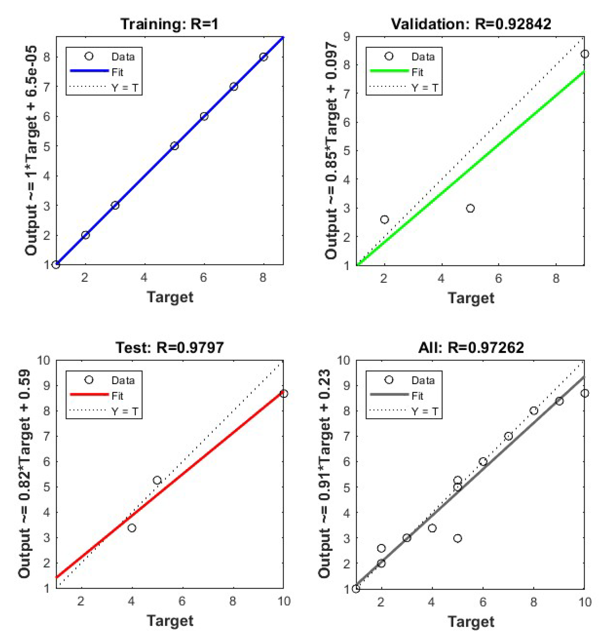
The regression analysis obtained from the different phases of NN (Figure 4) suggests that the model successfully translates the data to a validation point with a regression co-efficient (R2) valued at 0.97 while the same for Training, test and overall process are 0.96, 0.956 and 0.91 respectively.
Several outliers are visible in Figure 3, which are shown in the error histogram (Figure 5a). The figure is skewed on the right. This suggests that the inherent stochastic nature of the system is prone to shifting its equilibrium from the current stable state with the slightest perturbation, and, hence, is metastable. A similar outcome has been found in our previous work (Debnath et al. 2022).
Figure 5.
(a): Error Histogram and 5(b) Model performance obtained from NN.
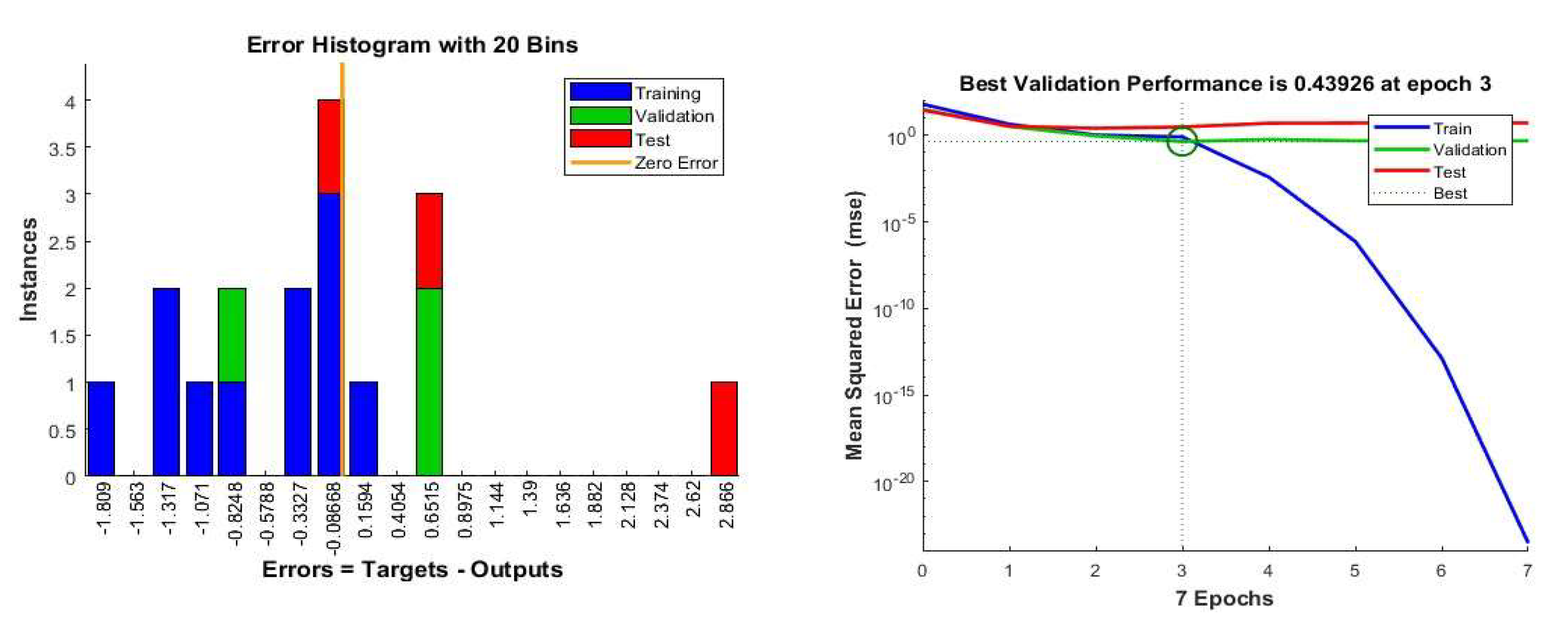
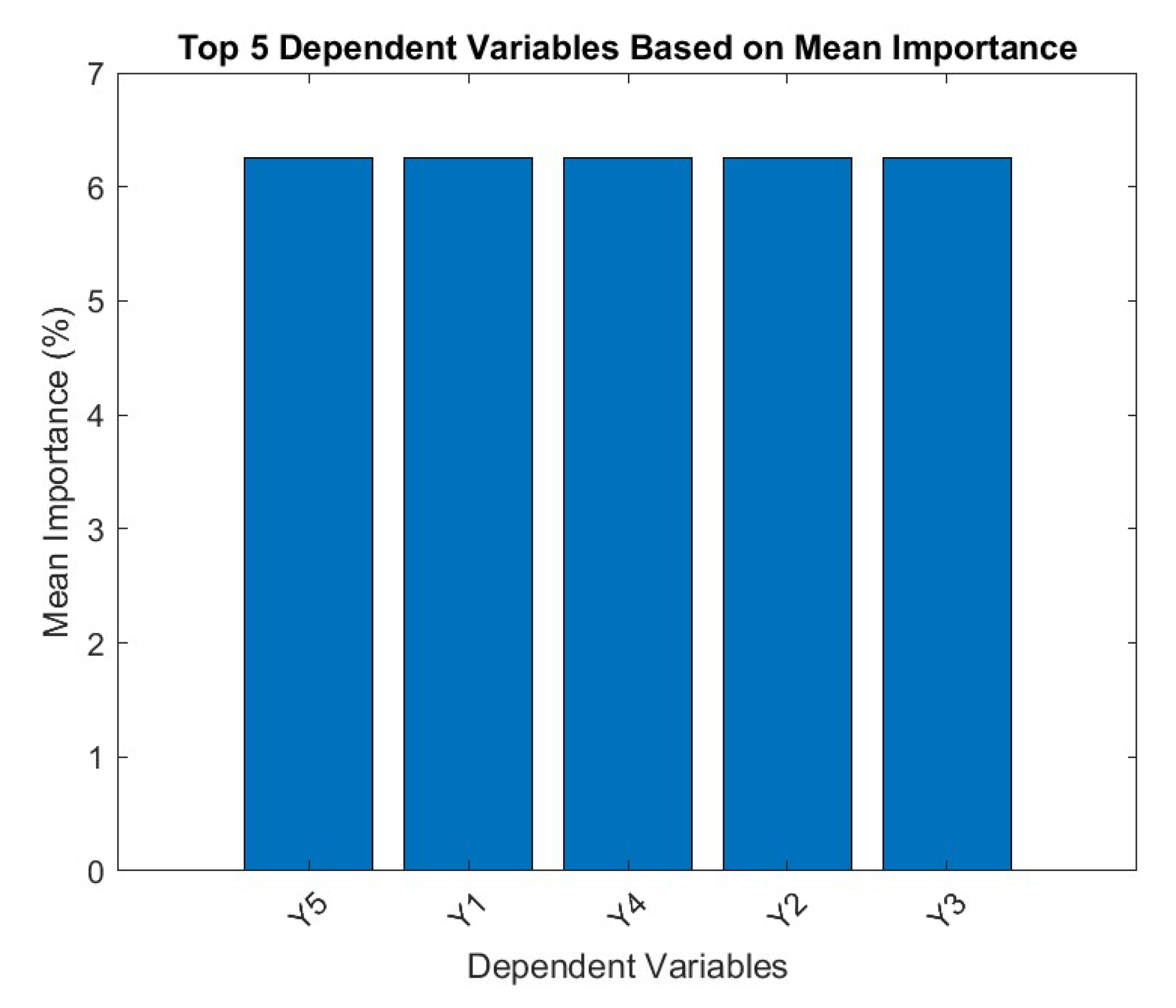
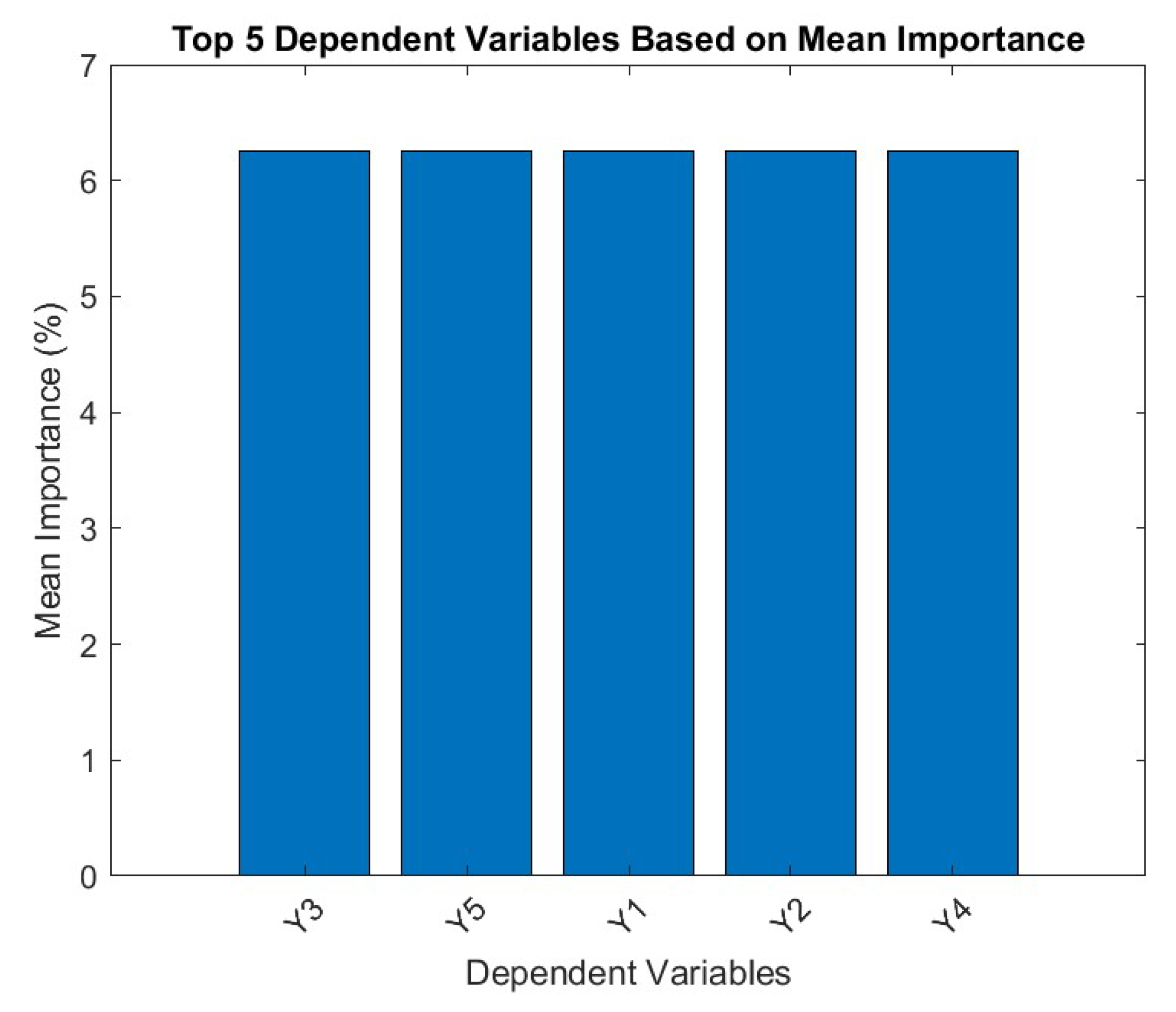
Figure 6.
Top 5 dependent variables based on Random Forest.
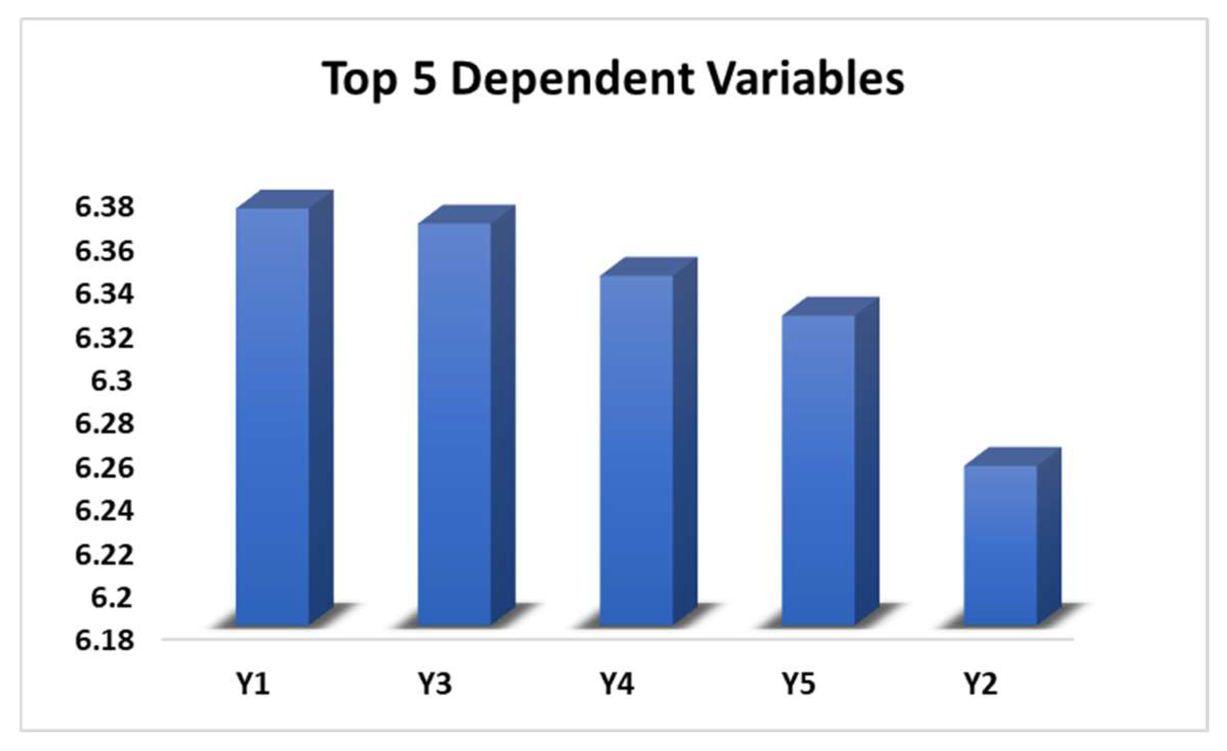
As can be seen, the Random Forest (RF) outputs are in partial agreement with the NN results. While the top three dependent variables in this case are Y1, Y3 and Y4 i.e., VCO2, Ww and Wp; Y2 here is the least important which is Ec and Y5 is the second least important i.e., N3. These results are somewhat the result of overestimation of the Random Forest algorithm, as in reality Y2 i.e., energy consumption is one of the sensitive parameters in the system (Debnath et al. 2024). However, given the nature of the e-waste recycling plant considered here which is primarily engaged in a mechanical recycling will have a largely consistent consumption of energy. From that perspective, the RF outputs are justified.
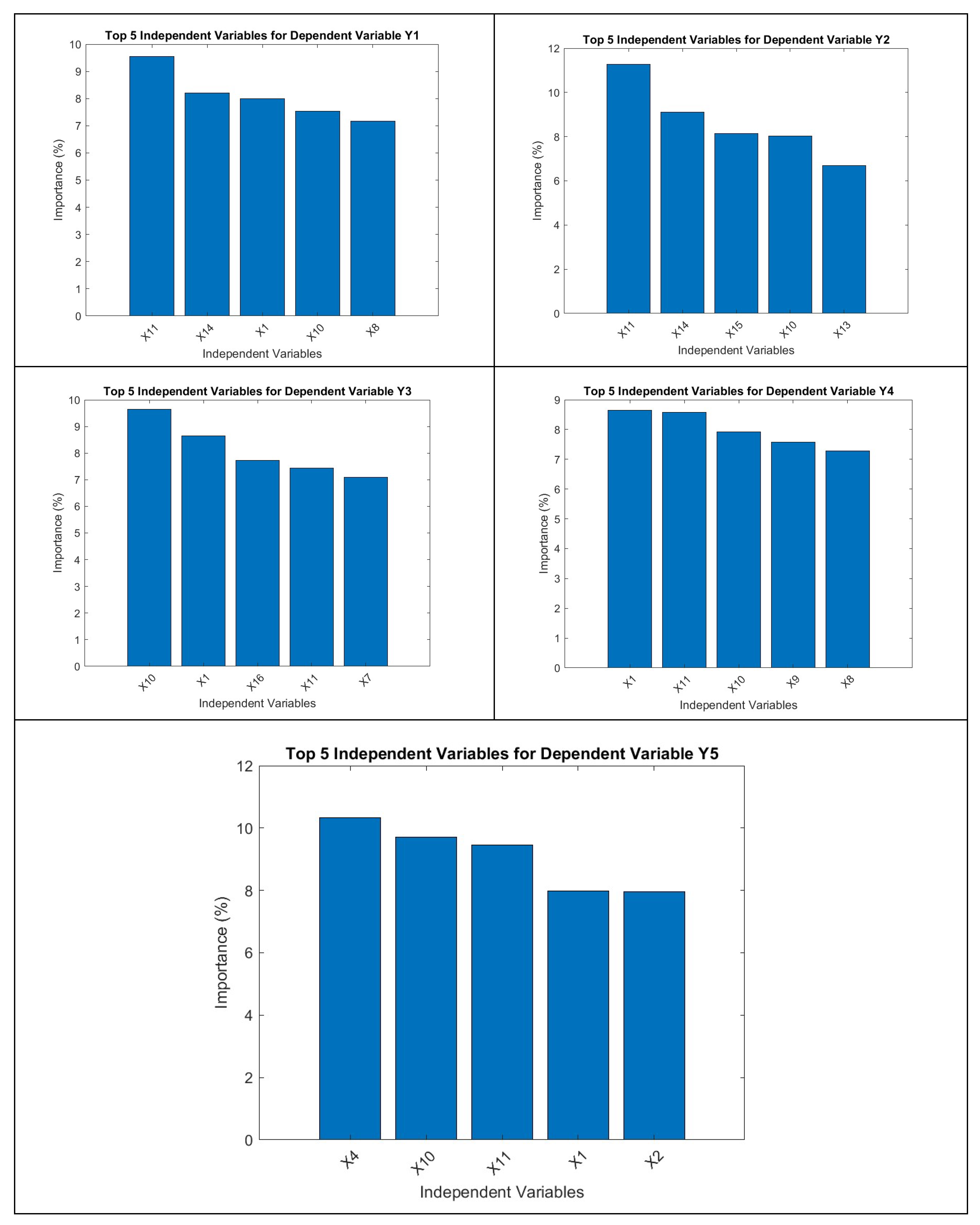
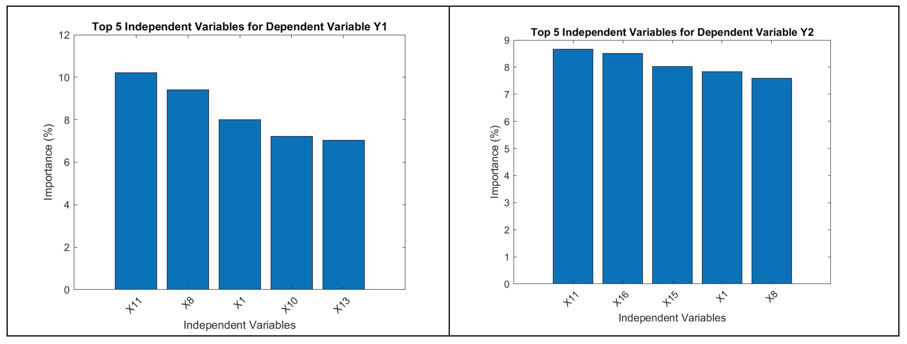
Figure 7.
a -d): Top 5 independent variables for dependent variable Y1, Y3, Y4 and Y5 from RF.
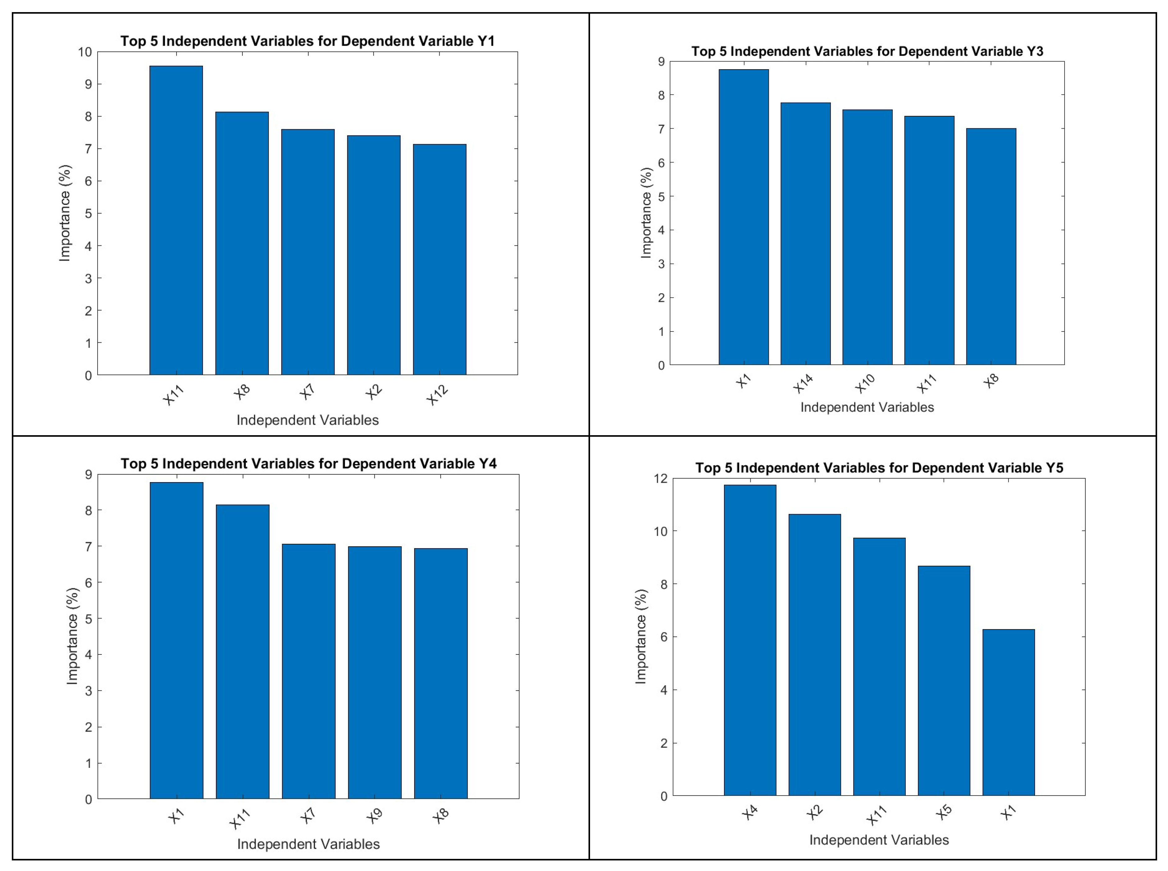
The RF algorithm takes things one step further with the estimation of the highest contributors (independent variables) to the top dependent variables. For Y1 i.e., VCO2 the top contributors are X11 (F5), X8 (F2), X7 (F1), X2 (N4) and X12 (F6) respectively. For Y3 i.e., Ww the top contributors are X1 (N1), X14 (F8), X10 (F4), X11 (F5) and X8 (F2) respectively. In case of Y4 i.e., Wp the top contributors are X1 (N1), X11 (F5), X7 (F1), X9 (F3) and X8 (F2) respectively. On the other hand, for Y5 i.e., N3 the top contributors are X4 (N7), X2 (N4), X11 (F5), X5 (N8) and X1 (N1) respectively. These results differ from NN outputs while revealing more intricate details.
3.2. Case 2: Perturbation in F4
Figure 8 represents the correlation between dependent and independent variables of the considered e-waste supply chain system with F4 inducing fluctuations. Independent variables 7 (F1), 9 (F3), 12 -16 (F6 – F8, F10 and F11) are highly sensitive having most of the complex effect to the dependent variables except no. 5 which is N3. On the other hand, independent variables 1-6 (N1, N4, N5, N7-N9), 8 (F2), 10 (F4) and 11 (F6) are least affected. Surprisingly, the results suggest that F4, which is the variable we have perturbed here, is the least affected. However, in the benchmark case, F4 was a sensitive variable. This change in the system is pushing the SCN towards a more equilibrium state rather than forcing it out of it, as one would expect.
From Figure 9, the top 4 dependent variables are clearly seen as Ww, N3, Wp and Ec. Although the overall importance of direction is negative, the magnitude confirms this initial analysis.
The regression analysis obtained from the different phases of NN (Figure 10) suggests that the model successfully translates data to a validation point with a regression co-efficient (R2) of 0.95 while the same for Training, test and overall process are 0.99, 0.96 and 0.94 respectively that are not too different from Figure 5.
Some outliers are visible in Figure 10 which are outlined in the error histogram, depicted in Figure 11a which is right-skewed. This suggests that the inherent stochastic nature of the system is prone to shifting its equilibrium from the current stable state with the slightest nudge. Similar outcome has been found in our previous work and consistent with the benchmark case (Debnath et al. 2022). Figure 11(b) illustrates a successful training process with the model achieving its best performance on validation data at epoch 3.
Figure 11.
a): Error Histogram and 11(b) Model performance obtained from NN.
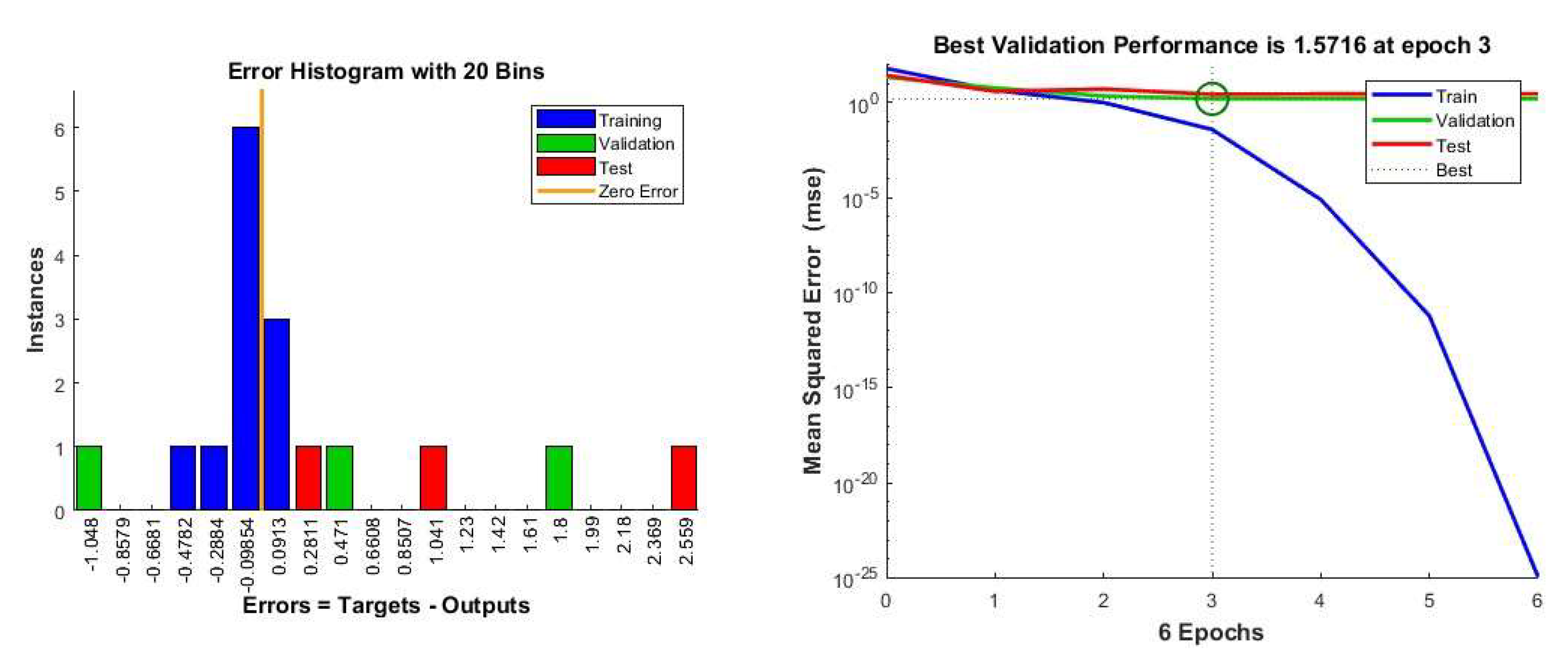
Figure 12.
Top 5 dependent variables based on Random Forest.
As can be seen, the Random Forest (RF) outputs, all dependent variables have equal mean importance which means either the algorithm is overpredicting or the system is exceptionally stable. The latter being a utopian scenario, it is more legitimate to consider the over predictive nature of the RF algorithm. Similar case of overprediction was found in our previous work with PCA (Debnath et al. 2024).
Figure 13.
a -e): Top 5 independent variables for dependent variable Y1, Y3, Y4 and Y5 obtained from RF.
Figure 13.
a -e): Top 5 independent variables for dependent variable Y1, Y3, Y4 and Y5 obtained from RF.
The RF algorithm takes things one step further with the estimation of the highest contributors (independent variables) to the top dependent variables. For Y1 i.e., VCO2 the top contributors are X11 (F5), X14 (F7), X1(N1), X10(F4) and X8 (F2) respectively. For Y2 i.e., Ec, the top contributors are X11 (F5), X14 (F7), X15(F10), X10(F4) and X13 (F7) respectively. For Y3 i.e., Ww the top contributors are X10 (F4), X1 (N1), X16 (F11), X11 (F5) and X7 (F1) respectively. For Y4 i.e., Wp, the top contributors are X1 (N1), X11 (F5), X10 (F4), X9 (F3) and X8 (F2) respectively. On the other hand, for Y5 i.e., N3 the top contributors are X4 (N7), X10 (F4), X11 (F5), X1 (N1) and X2 (N4) respectively. These results differ from NN outputs while revealing more intricate details.
3.3. Case 3: Perturbation in F7
Figure 14 represents the correlation between dependent and independent variables of the considered e-waste supply chain system. Independent variables 7 (F1), 9 (F3), 10 (F4), 12 (F6), 14 – 16 (F8, F10 and F11) are highly sensitive having most of the complex effect to the dependent variables except no. 5 which is N3. On the other hand, independent variables 1-6 (N1, N4, N5, N7-N9), 8 (F2), 10 (F4) and 12 (F6) are least affected. However, the green bar suggests that variable 1 i.e., N1 have significant effect on lead dependent variables.
Figure 14.
Correlation between Dependent and Independent Variables obtained from NN.
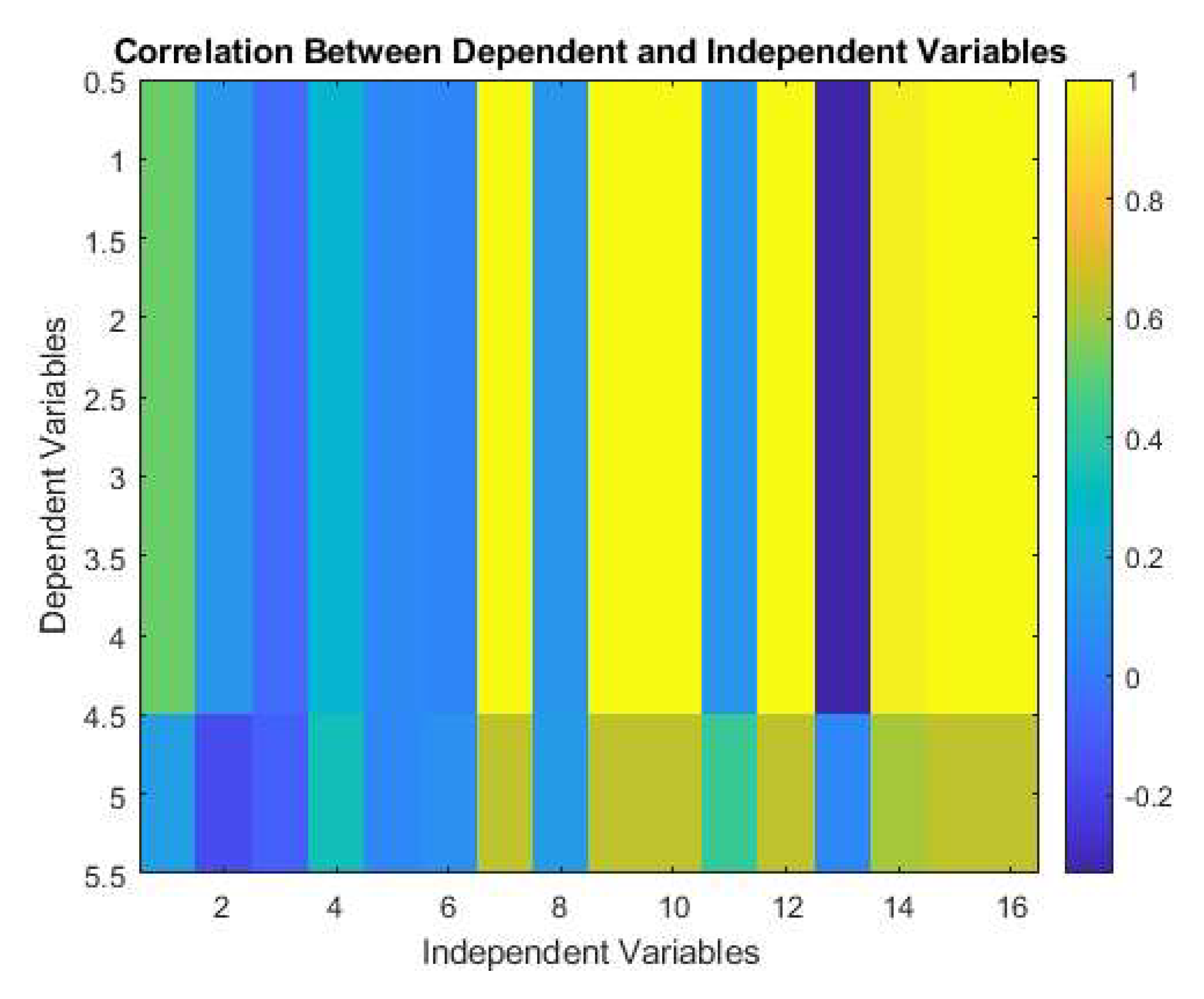
Figure 15.
Importance of the dependent variables obtained from NN.
The top 3 dependent variables are Ec, Ww and Wp. Positive values for these three dependent variables suggest that they have a significant effect on the e-waste supply chain. Considering, a Material Recovery from E-waste (MREW) plant aimed at recovering metals both via mechanical and chemical route (Debnath et al. 2018), energy consumption is going to be the most important parameter (Debnath et al. 2024a). In this case, the perturbed variable is F7 which is the revenue earned from selling the recycled materials recovered via e-waste treatment. Since the majority of the economic sustenance of any e-waste recycling plant is ploughed upon the material recovery efficiency and its market price, the results reconfirm the need for analyzing the stability of the model against market fluctuations in energy usage. As the results clearly depict that Ec is the most important variable here and the perturbed variable being F7 which is linked to the economic sustainability of the system, the need for optimization emerges as the most important variable. These findings are consistent with other experimental literature (Debnath et al. 2024b).
The regression analysis obtained from the different phases of NN (Figure 16) suggests that the model successfully translates the data to a validation point with a regression co-efficient (R2) of 0.93 while the same for Training, test and overall process are 1, 0.98 and 0.97 respectively. Once again, the error margins toe that of Figure 5 and Figure 10.
A few outliers are visible in Figure 16 which are captured in the error histogram and depicted in Figure 17a which is right-skewed. This suggests the inherent stochastic nature of the system which is prone to shifting its equilibrium from the current stable state. A similar outcome has been found in our previous work (Debnath et al. 2022). Figure 17(b) illustrates a successful training process with the model achieving its best performance on validation data at epoch 4.
Figure 17.
(a): Error Histogram and 17(b) Model performance obtained from NN.
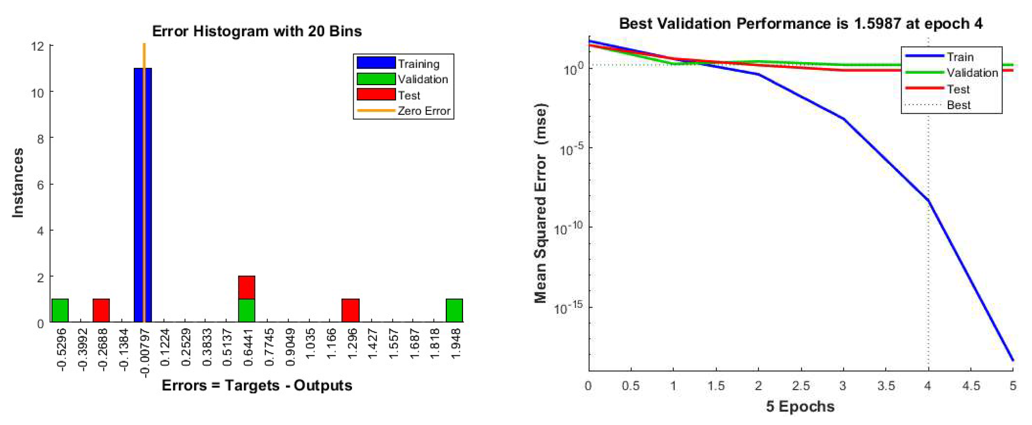
Figure 18.
Top 5 dependent variables based on Random Forest.
As can be seen, the Random Forest (RF) outputs, all dependent variables have equal mean importance which means either the algorithm is overpredicting or the system is exceptionally stable. The latter being a utopian scenario, it is more legitimate to consider the over predictive nature of the RF algorithm. Similar case of overprediction was found in our previous work with PCA (Debnath et al. 2024).
Figure 19.
(a -e): Top 5 independent variables for dependent variable Y1, Y3, Y4 and Y5 obtained from RF.
Figure 19.
(a -e): Top 5 independent variables for dependent variable Y1, Y3, Y4 and Y5 obtained from RF.
The RF algorithm takes things one step further with the estimation of highest contributors (independent variables) to the top dependent variables. For Y1 i.e., VCO2 the top contributors are X11 (F5), X14 (F7), X1(N1), X10(F4) and X8 (F2) respectively. For Y2 i.e., Ec the top contributors are X11 (F5), X14 (F7), X15(F10), X10(F4) and X13 (F7) respectively. For Y3 i.e., Ww the top contributors are X10 (F4), X1 (N1), X16 (F11), X11 (F5) and X7 (F1) respectively. In case of Y4 i.e., Wp the top contributors are X1 (N1), X11 (F5), X10 (F4), X9 (F3) and X8 (F2) respectively. On the other hand, for Y5 i.e., N3 the top contributors are X4 (N7), X10 (F4), X11 (F5), X1 (N1) and X2 (N4) respectively. These RF results differ from NN outputs while revealing more intricate details.
4. Conclusions
The study combined the deep learning recess of Deep Neural Network (NN) with a Random Forest Network (RFN) for extraction of relevant features from the dataset. Both models were effective in unmasking underlying patterns within the perturbed supply chain system which our earlier approaches (Debnath, et al. 2022; Debnath, et al. 2024a) were unable to predict. In the benchmark case, both NN and RFN extracted identical patterns, however in most cases, NN outperformed RFN. The superior performance of NN can be attributed to its ability to associate latent interactions and stratify information across kernels which is beyond the capability of RFN. This enables a nuanced dimension for deciphering and understanding the supply chain behavior. However, sometimes direct interpretability was overshadowed due to outliers leading to poor regression co-efficient.
On the contrary, the RFN was unable to clearly capture the effect of the dependent variables. Despite this, RFN could provide insights into the independent variables in the simulated uncertainty scenarios. Specifically, the effect of perturbing quasi-steady variables was more clearly captured in some cases. However, there were multiple scenarios where RFN over predicted due to complex interdependencies among the variables.
The juxtaposition of these two models reveals a trade-off between predictive power and interpretability. While the NN served as a potent tool for uncovering hidden complexity and emergent behaviors, the RFN proved invaluable for feature engineering, scenario simplification, and system pruning. This complementary use reinforces the importance of hybrid modelling approaches in supply chain analytics—particularly in domains characterized by uncertainty, feedback, and evolving equilibria, such as e-waste management networks. Note, the platform outlined is sufficiently generic to be repurposed beyond the present data regime and can be used to analyze different SCNs.
Author Contributions
Conceptualization, ZWN and BD; methodology, BD and AKC; software, ZWN; validation, ZWN, BD and AKC; formal analysis, BD and ZWN; investigation, BD and AKC; resources, ZWN and AKC.; data curation, ZWN; writing—original draft preparation, ZWN and BD; writing—review and editing, ZWN and AKC; visualization, ZWN and BD; supervision, AKC; project administration, ZWN; funding acquisition, ZWN. All authors have read and agreed to the published version of the manuscript.
Funding
This research received no external funding.
Data Availability Statement
Industry specific data are bound by non-disclosure clauses, but plots and codes may be made available by the corresponding authors on request.
Conflicts of Interest
The authors declare no conflicts of interest.
References
- Debnath, B., El-Hassani, R., Chattopadhyay, A. K., Kumar, T. K., Ghosh, S. K., & Baidya, R. (2022). Time evolution of a supply chain network: Kinetic Modeling. Physica A: Statistical Mechanics and its Applications, 607, 128085. [CrossRef]
- Goldstein, H., Poole, C. P., and Safko, J. In Classical Mechanics; Publisher: Pearson Education, 2011; ISBN: 978-813175891.
- Debnath, B., Chattopadhyay, A. K., & Kumar, T. K. (2024a). An economic optimization model of an e-Waste supply chain network: Machine learned kinetic modelling for sustainable production. Sustainability, 16(15), 6491. [CrossRef]
- Debnath, B., Chattopadhyay, A. K., & Kumar, T. K. (2024b). Cleaner Production in Multivariate Supply Chain Networks: Sustainable Business Future Through a “Roll of Dice”. In Circular Economy and Sustainable Development: A Necessary Nexus for a Sustainable Future (pp. 655-674). Cham: Springer International Publishing. [CrossRef]
- Debnath, B., Chowdhury, R., & Ghosh, S. K. (2018). Sustainability of metal recovery from E-waste. Frontiers of environmental science & engineering, 12, 1-12. [CrossRef]
- Mun, J. In Case Studies in Certified Quantitative Risk Management (CQRM): Applying Monte Carlo Risk Simulation, Strategic Real Options, Stochastic Forecasting, ... Business Intelligence, and Decision Modeling; ROV Press; ISBN: 978-1734497328.
- Breiman, L. (2001). Random Forests. Machine Learning, 45(1), 5-32. [CrossRef]
- Aggarwal, C, C. In Neural Networks and Deep Learning: A Textbook; Publisher: Springer; ISBN: 78-3319944630.
- Wang, J., Swartz, C. L., & Huang, K. (2023). Deep learning-based model predictive control for real-time supply chain optimization. Journal of Process Control, 129, 103049. [CrossRef]
- Jin, S., & Sun, X. (2025). Deep Neural Network Fusion Model for Accurate Logistics Demand Prediction of Agricultural Products. Journal of Circuits, Systems and Computers.
- de Carvalho Freitas, E. S., & Xavier, L. H. (2025). System dynamics applied to the e-waste value chain: A brazilian case study. Ecological Modelling, 506, 111139. [CrossRef]
- Vogt, L. (2025). Challenges in Closed-Loop Supply Chains: A Case Study of E-Waste Recycling Industries. Reports of Circular Economics, 1(1).
- Fuji, T., Ito, K., Matsumoto, K., & Yano, K. (2018). Deep multi-agent reinforcement learning using dnn-weight evolution to optimize supply chain performance. [CrossRef]
- Vairagade, N., Logofatu, D., Leon, F., & Muharemi, F. (2019). Demand forecasting using random forest and artificial neural network for supply chain management. In Computational Collective Intelligence: 11th International Conference, ICCCI 2019, Hendaye, France, September 4–6, 2019, Proceedings, Part I 11 (pp. 328-339). Springer International Publishing. [CrossRef]
- Farazi, M. Z. R. (2025). Building Agile Supply Chains with Supply Chain 4.0: A Data-Driven Approach to Risk Management. The American Journal of Engineering and Technology, 7(03), 21-34. [CrossRef]
- Gao, J., Adjei-Arthur, B., Sifah, E. B., Xia, H., & Xia, Q. (2022). Supply chain equilibrium on a game theory-incentivized blockchain network. Journal of Industrial Information Integration, 26, 100288. [CrossRef]
- Leong, W. Y., Wong, K. Y., & Anjomshoae, A. (2025). A systematic literature review of aggregate production planning (APP): Social and economic perspectives. Journal of Industrial Engineering and Management, 18(1), 48-71. [CrossRef]
- Bruni Prenestino, F., Barbierato, E., & Gatti, A. (2025). Robust Synthetic Data Generation for Sequential Financial Models Using Hybrid Variational Autoencoder–Markov Chain Monte Carlo Architectures. Future Internet, 17(2), 95. [CrossRef]
- Singh, A., Goel, A., Chauhan, A., & Singh, S. K. (2025). Sustainability of Electronic Product Manufacturing through E-Waste Management and Reverse Logistics. Sustainable Futures, 100490. [CrossRef]
- Klabunde, M., Schumacher, T., Strohmaier, M., & Lemmerich, F. (2025). Similarity of neural network models: A survey of functional and representational measures. ACM Computing Surveys, 57(9), 1-52. [CrossRef]
- Imani, M., Beikmohammadi, A., & Arabnia, H. R. (2025). Comprehensive analysis of random Forest and XGBoost performance with SMOTE, ADASYN, and GNUS under varying imbalance levels. Technologies, 13(3), 88. [CrossRef]
- Nweje, U., & Taiwo, M. (2025). Leveraging Artificial Intelligence for predictive supply chain management, focus on how AI-driven tools are revolutionizing demand forecasting and inventory optimization. International Journal of Science and Research Archive, 14(1), 230-250. [CrossRef]
- Kavil, Y. N., Alshemmari, H., Alkasbi, M. M., Alelyani, S. S., Orif, M. I., & Al-Farawati, R. K. (2025). Electronic waste and environmental diplomacy: How GCC E-waste management interfaces with the Stockholm Convention. Journal of Hazardous Materials Advances, 100610. [CrossRef]
- Choi, W. H., Pae, K. P., Kim, N. S., Kang, H. Y., & Hwang, Y. W. (2023). Feasibility study of closed-loop recycling for plastic generated from waste electrical and electronic equipment (WEEE) in South Korea. Energies, 16(17), 6358. [CrossRef]
- Campana, P., Censi, R., Ruggieri, R., & Amendola, C. (2025). Smart Grids and Sustainability: The Impact of Digital Technologies on the Energy Transition. Energies, 18(9), 2149. [CrossRef]
- Bhatnagar, B., & Dixit, V. (2025). Resilient supply chains: advancing technology integration with pre-and post-disruption technology roadmap. Journal of Enterprise Information Management. [CrossRef]
Figure 2.
Correlation between Dependent and Independent Variables obtained from NN.
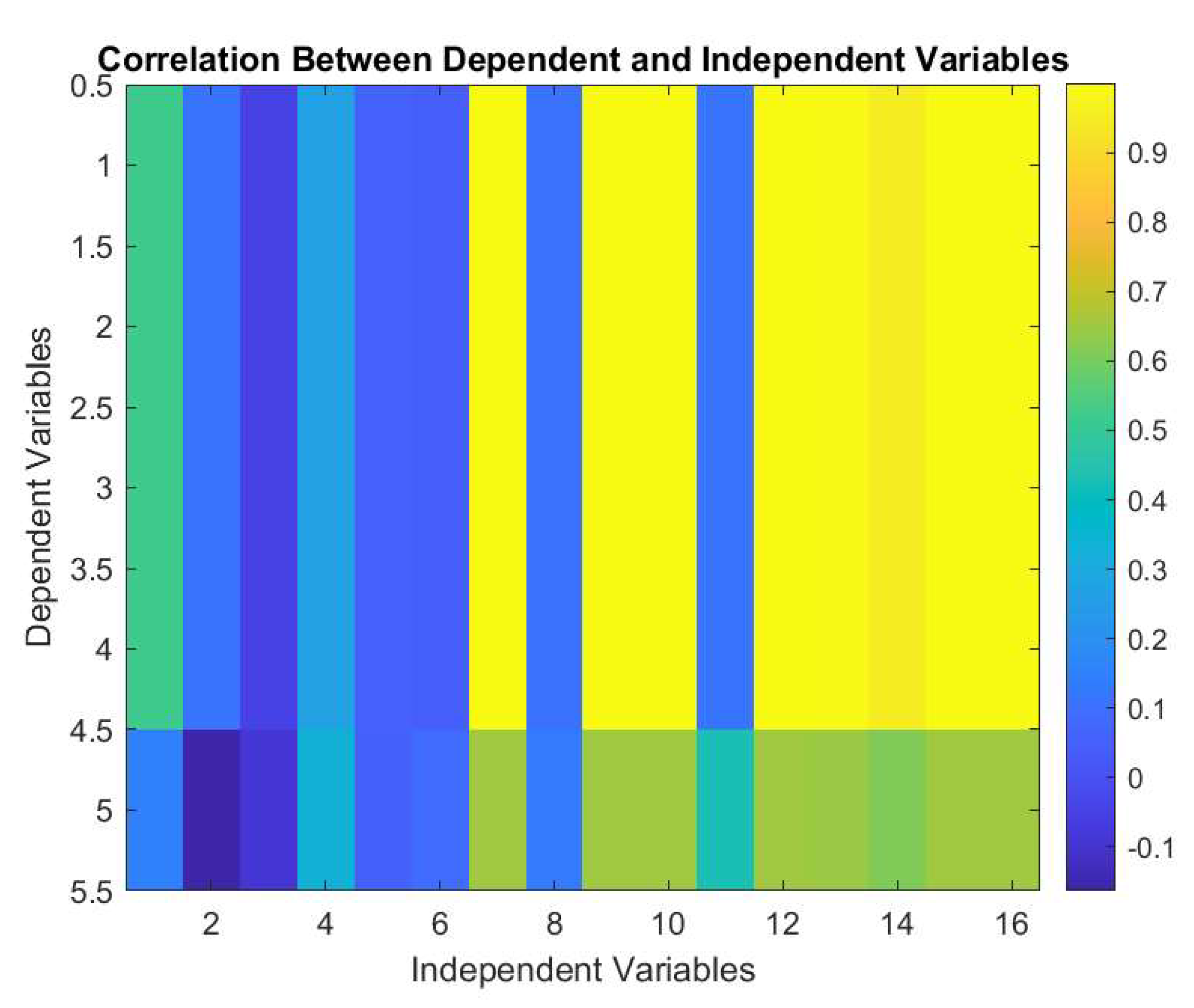
Figure 3.
Importance of the dependent variables obtained from NN.
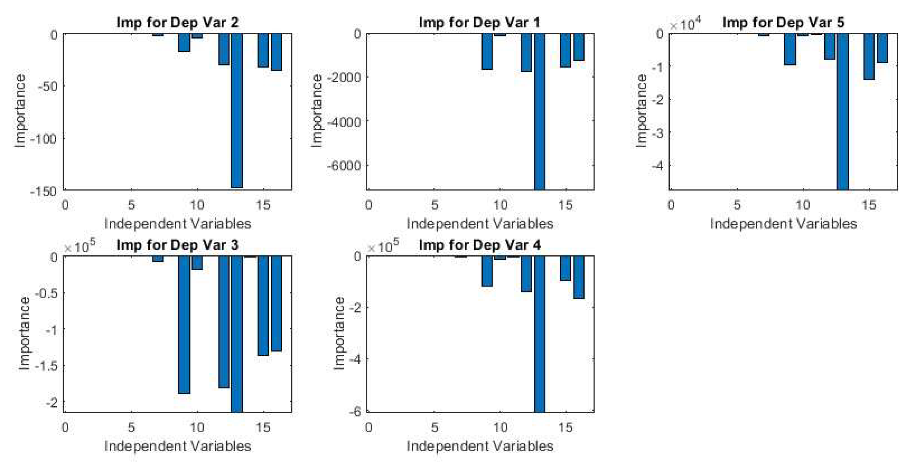
Figure 4.
Regression Analysis obtained from NN.
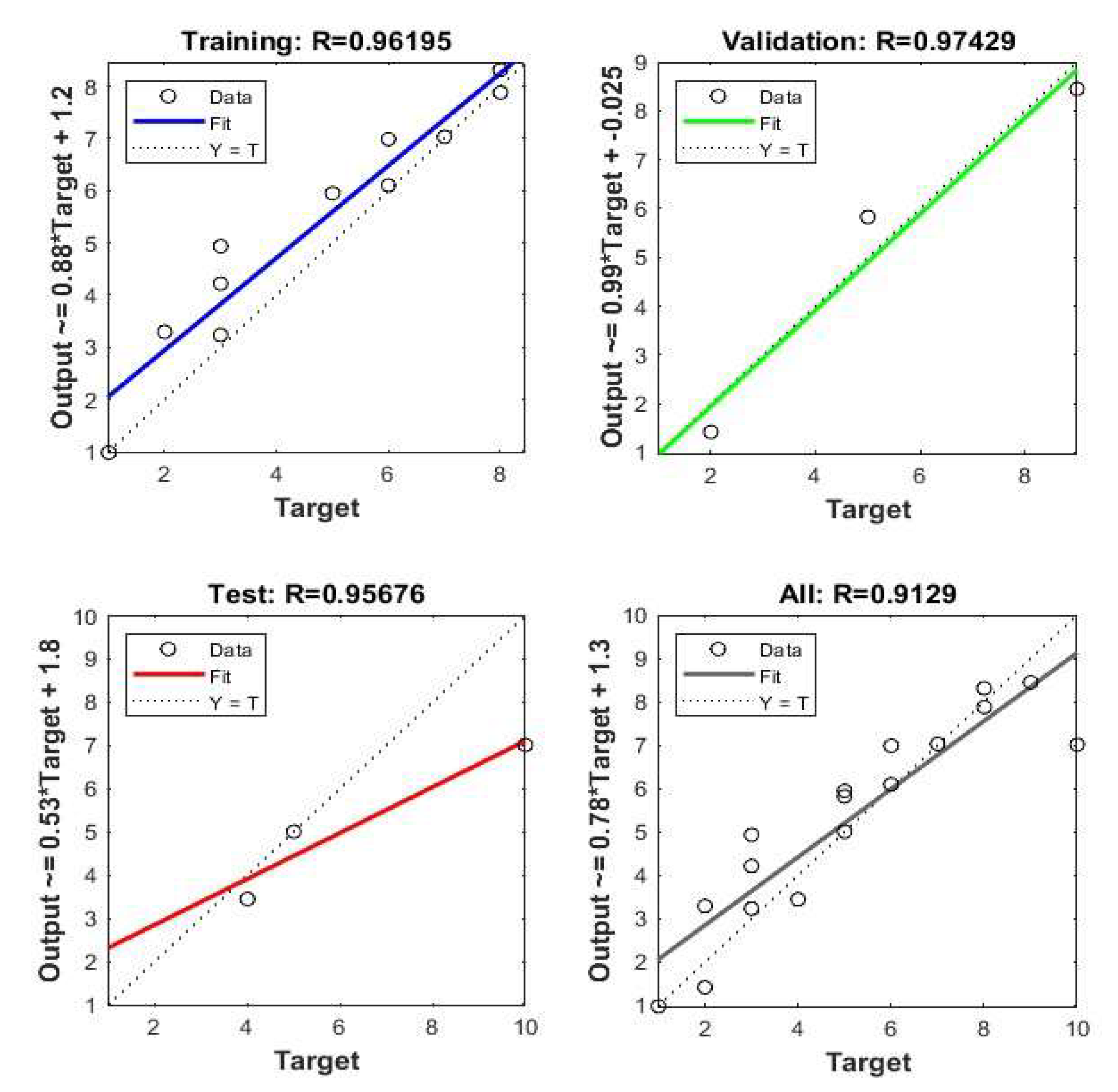
Figure 8.
Correlation between Dependent and Independent Variables obtained from NN.
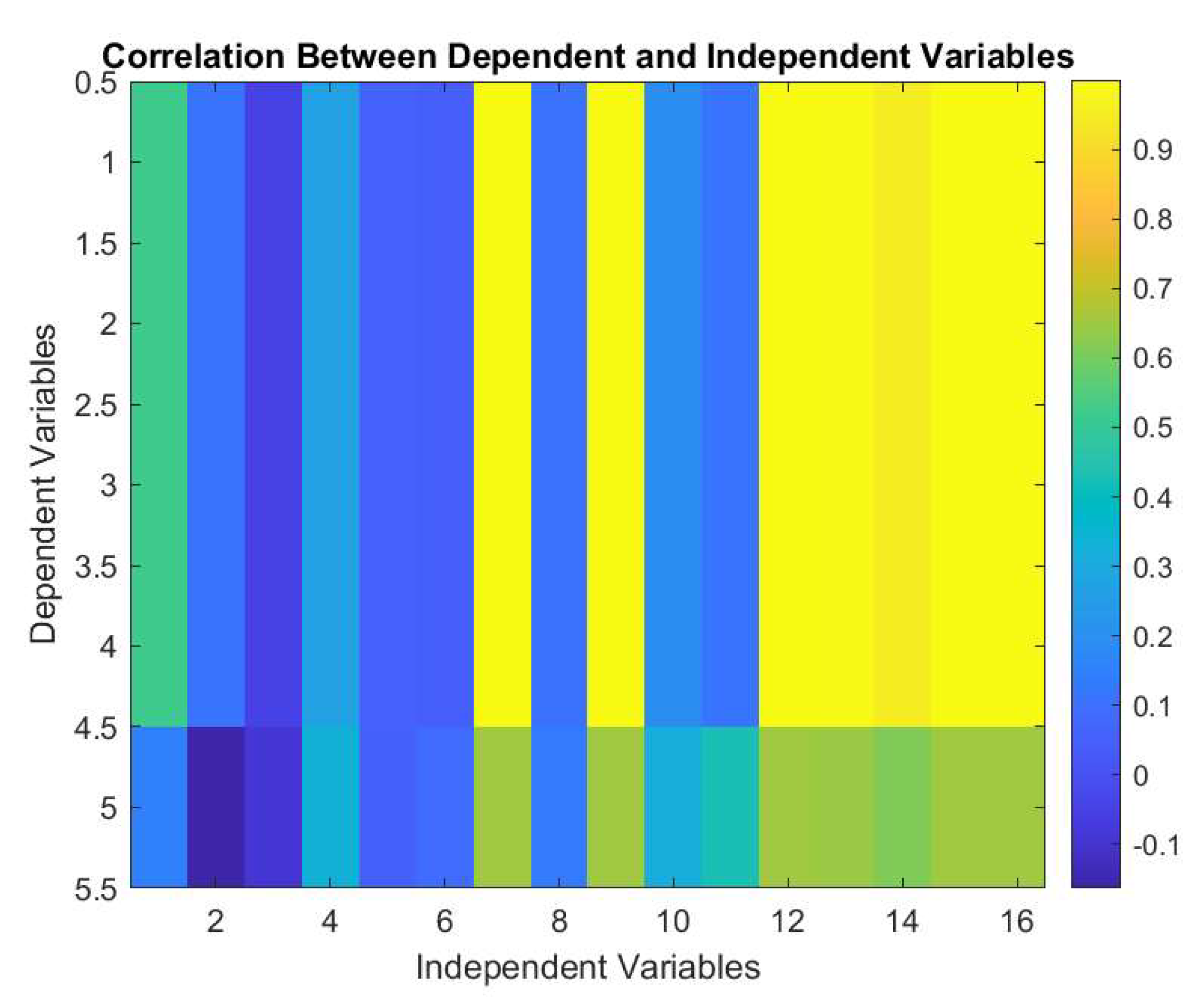
Figure 9.
Importance of the dependent variables obtained from NN.
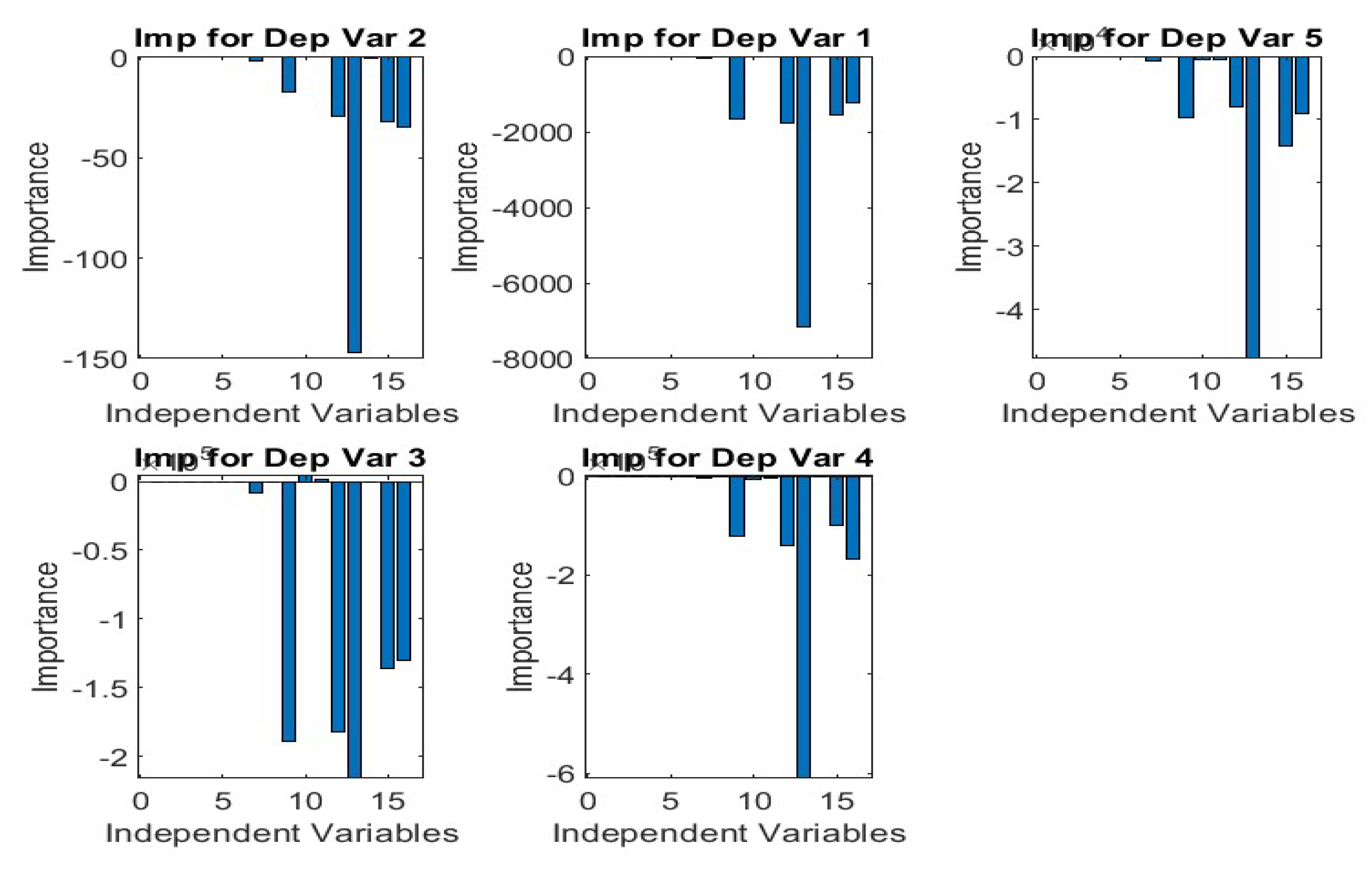
Figure 10.
Regression Analysis obtained from NN.
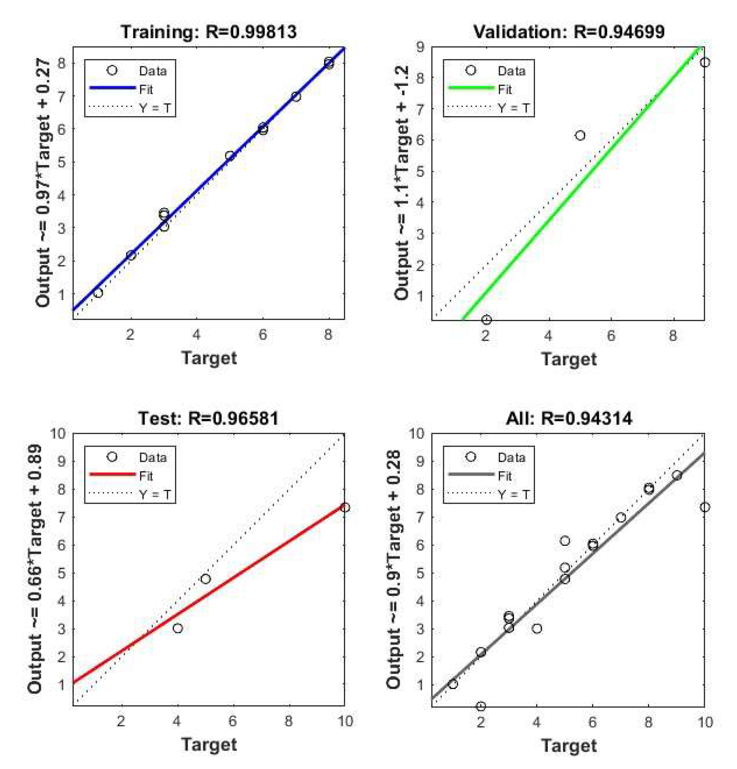
Figure 16.
Regression Analysis obtained from NN.
Disclaimer/Publisher’s Note: The statements, opinions and data contained in all publications are solely those of the individual author(s) and contributor(s) and not of MDPI and/or the editor(s). MDPI and/or the editor(s) disclaim responsibility for any injury to people or property resulting from any ideas, methods, instructions or products referred to in the content. |
© 2025 by the authors. Licensee MDPI, Basel, Switzerland. This article is an open access article distributed under the terms and conditions of the Creative Commons Attribution (CC BY) license (http://creativecommons.org/licenses/by/4.0/).
Copyright: This open access article is published under a Creative Commons CC BY 4.0 license, which permit the free download, distribution, and reuse, provided that the author and preprint are cited in any reuse.


