
Submitted:
28 May 2025
Posted:
29 May 2025
You are already at the latest version
Abstract
We aim to provide detailed derivation and analytical investigation that lead to closed-form mathematical equations that describe how various plasma properties (such as the electric conductivity and the travel speed) affect the resultant electric behavior of the plasma as a supersonic electrically conductive medium that flows under the influence of an applied magnetic field to produce direct current electricity within a linear channel. This magnetohydrodynamic problem can take four main forms, depending on the geometric design and electric connectivity of electrodes. Starting from basic principles and using informative sketches, we explain the equations governing the performance of this power generation technique, and contrast the operational conditions for the four different channel cases.
Keywords:
plasma
; electric
; supersonic
; applied mathematics
1. Introduction
1.1. Background
Electricity is a main driver for modern civilization [1,2,3,4,5,6,7,8]. Global electricity generation and demand have been generally increasing steadily since 2000, except for irregularities in 2009 due to the 2008 economic recession and in 2020 due to the COVID-19 pandemic [9,10,11,12]. While conventional power systems (i.e. power plants that burn fossil fuels [13,14,15,16,17,18,19]) are reliable methods for generating large amounts of electricity, their harmful GHG (greenhouse gas) emissions [20,21,22,23,24,25,26,27,28] and other pollutants encourage the shift to non-conventional alternatives, such as renewable energy sources [29,30](such as solar energy [31,32,33,34,35,36], wind energy [37,38,39], and crop-based bioenergy [40]), and low-carbon hydrogen [41,42,43,44,45].
Another method for non-conventional electricity generation is the magnetohydrodynamic (MHD) generator [46]. Such generators utilize the Lorentz force and electromagnetic principles to extract energy from a moving ionized gas (plasma) to produce direct current (DC) electricity without rotating or reciprocating elements as found in conventional heat engines [47,48,49,50].
There are two broad categories of MHD generators. One category of MHD generators is the open-cycle generators, where combustion products (such as carbon dioxide “CO2” and steam “H2O”) are seeded with alkaline compounds (e.g. potassium carbonate “K2CO3”), and they form weakly-ionized thermal (equilibrium) plasma that is accelerated within a channel while subject to a magnetic field to induce electric fields and electric currents [51,52]. Such a channel may be viewed as an “electromagnetic turbine”. Being in thermal equilibrium (or thermodynamic equilibrium) means that the electrons (the effective charge carriers due to their light mass and thus high mobility) and the heavy particles in the plasma gas (ions, atoms, and molecules) in such combustion plasmas can be treated as having one common temperature due to the high collision frequencies and high energy transfer per collision [53,54]. Being open-cycle means that the working plasma is not recirculated back after energy is extracted from it for electricity generation.
The other broad category of MHD generators is the closed-cycle type, in which MHD generators utilize a heated inert gas (e.g. argon “Ar”) [55,56] whose temperature is elevated using a heat exchanger (rather than a direct combustion process), and this heated gas is seeded with an alkaline metal, such as cesium vapor (Cs) to form a non-equilibrium plasma medium. It should be noted here that the alkali metal cesium, which has an atomic number of 55, vaporizes at a relatively low temperate of about 944 K (671 °C) [57,58], while it readily melts near room temperatures at only 302 K (29 °C) [59,60]. Being a non-equilibrium plasma means that its constituent gas particles (electrons, ions, atoms, and molecules) are not in a state of thermal equilibrium, with electrons characterized by a higher temperature compared to heavy particles (ions, atoms, and molecules) [61,62]. The higher temperature of electrons in inert gas plasmas is necessary for keeping a sufficient level of electric conductivity despite the relatively low bulk temperatures. This state of non-equilibrium (two-temperature plasma) can be achieved by ohmic heating (Joule heating) under a relatively small frequency of collisions between the electrons and the neutral gas atoms [63,64]. Being closed-cycle means that the working plasma is recirculated back after energy is extracted from it for electricity generation. Before repeating the energy extraction process, energy is added again to the depleted plasma (e.g. by a heat exchanger) to restore its initial state [65].
Closed-cycle magnetohydrodynamic (CCMHD) generators typically have a disc shape [66,67,68,69,70], and this design allows efficient utilization of the magnets [71]. The compactness of CCMHD generators renders them of special interest in space applications, especially in space missions reaching trajectories far from the sun, where solar irradiation and photovoltaic power conversion become ineffective [72].
On the other hand, open-cycle magnetohydrodynamic (OCMHD) generators pertain more to terrestrial electricity generation; where they can provide much larger production capacities. Such OCMHD generators may be used either in a continuous mode as power plants or in a pulsed mode for geological prospecting.
First, we have the enthalpy extraction or enthalpy extraction ratio () metric, which is the ratio of the drop in static enthalpy () within the MHD generator to the inlet static enthalpy () at the entrance of the MHD generator. Thus,
where () and () are the specific static enthalpy of the plasma at the entrance and at the exit of the MHD generator. A high enthalpy extraction () of 38% was successfully demonstrated experimentally for a disc-type MHD generator [75].
Second, there is the MHD generator isentropic efficiency () [76], which relates the actual relative drop in the static enthalpy to the ideal relative drop in the total (stagnation) enthalpy () in the case of an isentropic process under the assumption of a calorically-perfect gas (thus, having constant specific heat capacities and constant specific heat ratio) [77,78,79,80,81]. This MHD isentropic efficiency is
where () is the specific total enthalpy of the plasma at the entrance of the MHD generator.
The above equation can be written in terms of the total pressure (the stagnation pressure, which is the sum of the static pressure and the dynamic pressure [82]) at the entrance of the MHD generator () and at the exit of the MHD generator () using standard expressions for isentropic compressible calorically-perfect flows [83] as
where () is a constant specific heat ratio (ratio of the specific heat capacity at constant pressure to the specific heat capacity at constant volume). A high MHD isentropic efficiency () of 63% was successfully demonstrated experimentally for a disc-type MHD generator [84].
Third, there is the MHD generator electric (), which is defined as the ratio of the electric power to the mechanical power. Mathematically, this is expressed as
Open-cycle magnetohydrodynamic (MHD) generators are primarily in the form of a linear channel, in which the weakly-ionized plasma moves at a high speed while subject to a strong applied magnetic field [85]. The inlet plasma speed can be subsonic (Mach < 1) [86,87,88] or supersonic (Mach > 1) [89,90,91,92,93,94,95,96,97]. Contrary to subsonic and incompressible flows [98,99,100,101,102,103,104,105,106,107,108,109], supersonic flows at the MHD channel entrance need a divergent MHD channel in order to allow the supersonic flow to expand and accelerate [110,111,112]. Attached electrodes are used to transmit the collected electric current to an external eclectic load. There are four common designs for the open-cycle MHD channels; namely, (1) continuous-electrode Faraday channel [113,114,115], (2) segmented-electrode Faraday channel [116,117,118], (3) linear Hall channel (always have segmented electrodes) [119,120,121], and (4) diagonal channel or diagonal-electrode channel or diagonally-shorted channel (always have segmented electrodes) [122,123,124]. Each of these designs has a unique layout of its electrodes, hence the name of its type.
1.2. Goal of the Study
This work can be viewed as an extension of our earlier studies about mathematical modeling for magnetohydrodynamic (MHD) power generation. We previously presented the governing electric equations in the MHD channel under various levels of modeling approximation [125]. We also proposed three mathematical approaches for resolving the electric field within the MHD domain [126]. In addition, we discussed a mathematical model for relating the electric conductivity of MHD plasma with its local temperature, pressure, and chemical composition [127].
In continuation to our work about mathematical modeling for magnetohydrodynamic (MHD) generators, we here aim to present mathematical expressions for the electric field and electric current-density field within the plasma of an open-cycle MHD generator, and the resulting output power density under the four types of linear MHD channels [128]. We supplement the mathematical analysis with illustrative sketches and logical derivation starting from elementary equations.
Our review of these mathematical expressions here and organized presentation and contrasting have a number of benefits. First, they serve as a guide for readers interested in open-cycle MHD (OCMHD) power generation and the difference in their performance according to the different channel configurations. Second, our review provided here involves explicit algebraic scalar expressions, enabling parametric and visual investigation of the nonlinear influence of some parameters on various variables of importance in the OCMHD channel [129,130,131]. For example, the penalty in the electric output power density () due to the Hall parameter () in the case of a continuous-electrode Faraday channel can be easily identified through the presented mathematical expressions in the current study. Third, the directions of the vector fields under each channel configuration are clarified, and this is useful in understanding the operation of the MHD generator for each case, and can help in optimizing or controlling the performance [132,133,134,135]. For example, the load factor in the linear Hall channel can be optimized for maximum power output through the presented mathematical expressions in this study. Fourth, the content of this study may be used in an educational environment [136,137,138,139,140,141,142,143], where students are exposed to the application of mathematics in an interdisciplinary subject this combines electric engineering, energy engineering, and physics [144]. The analysis presented here is simple, and can be viewed as reduced-order modeling [145] that takes advantage of a set of assumptions such that no computationally-demanding solutions of the partial differential equations using computational fluid dynamics (CFD) are needed [146,147,148,149,150,151].
2. Research Method
The method followed in the current study is the symbolic mathematical manipulation of a fundamental generic equation for electrically-conducting moving plasma. This equation is the generalized (extended) Ohm’s law in its vector form, which accounts for the Hall effect (Hall current-density) as well as the electromagnetic induction effect (Faraday current-density).
We expand this vector equation into three scalar equations (corresponding to the three Cartesian components). Then, we apply our assumptions to deduce two scalar equations for the axial component (along the plasma’s travel direction) and the vertical components (perpendicular to the magnetic field and the plasma velocity). We drop the third scalar equation (in the direction of the magnetic field) because it becomes trivial in our case.
These two derived scalar equations are analyzed further for each of the four linear channel configurations; and this leads to the aimed mathematical expressions for the electric field, electric current-density, and power density for each configuration.
The common assumptions made in this study are:
- The MHD channel has a divergent geometry, with a trapezoidal cross-section (in the plane). Such a simple MHD channel has been realized in the Sakhalin pulsed MHD generator [152,153,154]. The width (along the magnetic field) is constant, and its influence is disregarded here (this is equivalent to assuming infinite width, thus two-dimensional channels).
- The charge carriers are only the free electrons in the plasma (liberated as a result of thermal ionization). This means that while ions also exist (to ensure the overall neutrality of the plasma), their contribution to the electric current is neglected [155,156]. This is a reasonable assumption given the much stronger mobility of the lighter electrons compared to the heavier ions [157,158,159].
- Unidirectional magnetic field (magnetic-field flux density) that points in the positive >-axis. Therefore, the magnetic-field flux density vector () can be expressed as , where () is a unit vector in the direction of the positive -axis. Because the magnetic field is externally applied, this assumption can be justified. In such a case, special electromagnetic designs can be made to approximate this assumption. This treatment of the magnetic field as being fully controllable implies a low magnetic Reynolds number assumption [160,161,162,163], where auxiliary induced magnetic-field flux density due to the moving plasma (the self-excitation phenomenon) is neglected [164,165,166,167]. This “inductionless” assumption [168] of a low magnetic Reynolds number is reasonable for MHD generators [169,170,171].
- Unidirectional plasma velocity that points in the positive -axis. Therefore, the plasma velocity vector () can be expressed as , where () is a unit vector in the direction of the positive -axis. Although this assumption neglects turbulence and no-slip effects in the plasma flow, it can be regarded as an acceptable treatment for deriving system-level laws, where the time-averaged bulk velocity of the plasma should be primarily in the axial direction. This assumption becomes more valid when the divergence angle of the channel decreases, so the channel height approaches uniformity. In addition, turbulence tends to be suppressed as the Mach number increases [172,173]; and our study is for supersonic channels. In addition, adopting a one-dimensional approximation for a channel flow or exterior flow has been implemented in other studies [174,175,176,177].
- No electric field along the lateral direction (along the direction of the magnetic field). This assumption is aligned with the unidirectionality assumption for the magnetic field. Even if the plasma has a three-dimensional flow velocity, the unidirectional magnetic field along the -axis is not able to induce an electric field in the same -direction. Therefore, the electric field along the -axis within the MHD plasma can only be caused by an externally applied electric field; but such a case is not considered in the current study, where there are no electrodes along the -axis to permit this.
3. Base Scalar Equations for Electric Fields in MHD Plasma
In this section, we derive the two base scalar equations for the conventional electric current-density and the load-consumed electric field, under the assumptions made in the previous section; particularly the unidirectional magnetic field and the unidirectional plasma velocity. These scalar equations are the -component and the -component of the generalized Ohm’s law, which applies to a three-dimensional conductor medium (rather than a conductive wire).
The generalized Ohm’s law (for plasma with neglected ion drift) relates the electric current-density () to the electric field (), electric conductivity (), and the applied magnetic field () [178,179,180]. It should be noted that we adopt the conventional current here, rather than the electron current [181,182,183]. The only difference if the electron current is adopted rather than the conventional current is that the electric current-density () should have a minus sign in each appearance for it in our presented mathematical formulations.
The generalized Ohm’s law can be expressed in different forms, we start with the following convenient form for it, which facilitates our discussion and subsequent analysis:
where () is the electron mobility.
The Hall parameter () is the electron mobility () divided by the magnitude of the applied magnetic-field flux density (). Mathematically, this is expressed as
It is useful to add here that the electric conductivity of the plasma () due to the free electrons (ions contribution is neglected as mentioned earlier) is [184,185,186]
where () is the number density of the charge-carrier electrons, and () is the elementary charge (the absolute electric charge of an electron; [187,188,189]).
Therefore, the generalized Ohm’s law form in Equation (5) can be expressed in an alternative form as
where () is a unit vector in the direction of the applied magnetic-field flux density vector (). Thus, this unit vector is defined as
The first term in Equation (8), the term (), is an extended version of the classical Ohm’s law for a one-dimensional solid conductor. To demonstrate this; one can multiply both sides of the equation by the area () perpendicular to the electric current-density, and then replace the vector electric field () by the negative value of the scalar gradient of the electric potential (). This gives
where () is the magnitude of the unidirectional current density; and () is a numerical approximation for the gradient of the electric potential (), and it becomes exact in the case of a linear decrease of the electric potential in the direction of the conventional electric current density.
The product () in the above equation is the electric current ().
Also, the quantity () is the reciprocal of the resistance () of the conductor. Therefore,
Using Equation (11) and Equation (12) in Equation (10) gives the classical Ohm’s law, as
The minus sign in the above equation indicates that the electric potential drops in the direction of the electric current. This minus sign is normally dropped when Ohm’s law is expressed, with the understanding that the electric potential drops across the conductor or the load.
The second term in Equation (8), the term (), is the Hall electric current-density due to the Hall effect, where an electric voltage is induced as a result of the movement of the electrons under the effect of the applied magnetic field, and this leads to a “secondary” Hall current density perpendicular to both the “primary” current density () and the applied magnetic field () [190,191,192]. The magnitude of this “secondary” or Hall current density,, is proportional to the Hall parameter (). Thus, from Equation (6), The magnitude of this “secondary” or Hall current density,, is proportional to either the magnitude of the applied magnetic field () or the electron mobility ().
In the current study, the applied magnetic-field flux density vector is assumed to be totally in the -axis, whose unit vector is (). Therefore, we have
Using Equation (14) in Equation (8) gives a third form for the generalized Ohm’s law, which is
The cross product () leads to a vector that has two non-trivial components in the -axis and -axis only, as
Using Equation (16) in Equation (15), and collecting terms for the three Cartesian components gives the following three scalar equations:
Given that the -component of the within-channel electric field vector () is zero here
then, Equation (19) implies also that the -component of the electric current-density is zero
Equation (17) and Equation (18) are implicit expressions for the-component and the -component of the electric current-density, and these two components ( and ) are clearly coupled. However, these two coupled equations can be solved simultaneously to obtain two explicit uncoupled expressions for these two components ( and ), with the result being as follows:
The electric field vector within the plasma () is the vector sum of the electric field source vector or the open-circuit electric field vector () that is induced due to the motion of the electrically-conductive plasma under the effect of the applied magnetic field vector, and the electric field sink () that is consumed by the external electric load (if a load is connected). Thus,
The load electric field () in MHD power generation is dependent on the connected load. However, if the MHD channel is used in a reverse mode as a plasma accelerator (a magnetohydrodynamic drive), then this electric field () can be then viewed as an applied one, and the electric current is applied to the MHD electrodes from a powerful external DC (direct current) source, rather than being collected from the MHD electrodes [193,194,195].
The induced or convection open-circuit electric field vector () is related to the bulk velocity of the plasma () and the applied magnetic field vector (), while being perpendicular to both of them [196,197]. Thus,
From the two previous equations, Equation (24) and Equation (25), we can write the following:
For our case of unidirectional magnetic field () and unidirectional convective plasma velocity (), the -component and the -component of the above vector equation are
Using the above two expressions for () and () in Equation (22) and Equation (23) gives
These two scalar expressions are to be analyzed further and their customized form is to be discussed for each case of the four designs of the linear magnetohydrodynamic (MHD) channels. This is presented in the next four sections, with one section dedicated to each channel design.
In the case of Faraday-type MHD linear channels (the continuous-electrode version or the segmented-electrode version), it is the -component of the current density () and load electric field () that are useful because these are the current densities effectively collected by the channel electrodes (the anode and cathode, which are separated vertically “along the -axis”). In such cases, a Faraday load factor () can be introduced as the ratio of the load electric field () to the induced electric field (). So, mathematically we have
Equivalently, this Faraday load factor can be viewed as the ratio of the electric resistance of the load () to the total series resistance encountered by the electric current flow due to both the external electric resistance of the load and the effective internal electric resistance within the MHD generator itself that is designated by the symbol () (this internal resistance is caused by the bulk plasma region, the boundary layer near the wall [198,199], and any solid slag layer formed on the electrodes [200,201]). Therefore, the Faraday load factor () can be mathematically described as
Therefore, the Faraday load electric field () can be expressed as
The value of () is bounded between 0 and 1. At the extreme condition of , the circuit is open (the external load is disconnected). This corresponds to setting the load resistance to infinity () in Equation (32). At the other extreme condition of , the circuit is shorted (the external load is replaced with a perfect electric conductor). This corresponds to setting the load resistance to zero () in Equation (32). It can be shown that maximum power delivery to the “matched” external load occurs at an optimum Faraday load factor of [202,203].
In general, the direct current (DC) electric power delivered to the load powered by a magnetohydrodynamic channel is [204]
where () is an infinitesimal volume element.
The direct current (DC) electric power delivered to the load in the case of a Faraday-type MHD generator per unit volume of plasma is
where is the absolute value of the vertical “i.e. parallel to the -direction” current density (since it actually has a negative value due to pointing in the negative -direction).
In the case of Hall-type linear MHD channels, it is the -component of the current density () and load electric field () that are useful because these are the current densities effectively collected by the channel electrodes (the anode and cathode, which are separated axially “along the -axis”). In such cases, a Hall load factor () can be introduced as the ratio of the load electric field () to the induced (open circuit) axial electric field (). So, mathematically we have
where is the absolute value of the axial load electric field (since it is actually having a negative value due to pointing in the negative -direction).
As in the case of the Faraday load factor, the Hall load factor can be viewed as the ratio of the electric resistance of the load () to the total series resistance encountered by the electric current flow due to both the external electric resistance of the load and the effective internal electric resistance within the MHD generator itself (). Therefore, the Hall load factor () can be mathematically described as
Therefore, the absolute value of the Hall load electric field () can be expressed as
As in the case of the Faraday load factor, the value of () is bounded between 0 and 1. At the extreme condition of , the circuit is open. At the other extreme condition of , the circuit is shorted. Maximum power delivery to the “matched” external load occurs at an optimum Hall load factor of [205].
The direct current (DC) electric power delivered to the load in the case of a linear Hall MHD generator per unit volume of plasma is
4. Continuous-Electrode Faraday Channel
The first MHD channel design we review in this study is the continuous-electrode Faraday configuration. This is the simplest configuration among the four linear MHD channels in terms of physical construction and electric connectivity.
Using Equation (33) in Equation (29) and Equation (30) gives a customized form for the electric current-density components suitable for Faraday-type channels as
In Figure 1, we illustrate the geometric layout of this channel in the plane. The top side represents the anode electrode, which has a negative (or grounded) polarity. The bottom side represents the cathode electrode, which has a positive polarity. In this sketch, the channel height (the separating distance between the two electrodes) is assumed to increase linearly with the axial distance (). This is not necessary, and nonlinear profiles are permitted as well [206]. However, in the shown linearly-divergent channel, the equipotential surfaces (the virtual surfaces with constant electric potential ) become flat planes (straight lines in the shown two-dimensional sketch). These potential planes are projected in the plane as inclined straight lines, with their inclination gradually change from being coincident with the anode at the top to being coincident with the cathode at the bottom. In our sketch, we provide arbitrary values for sample intermediate equipotential lines, in addition to the top anode (which is also an equipotential line), and the bottom cathode (which is an equipotential line). We assign an electric potential of 30 V to the cathode, and a reference zero potential to the anode. These are not realistic values because they are small (actual cathode potential can exceed hundreds of volts [207,208,209]), but they are provided just to improve the explanation through numerical examples.
The -component of the load electric field () is positive in the case of the continuous-electrode Faraday channel, meaning that it is pointing vertically up, from the bottom positive cathode to the top negative (or grounded reference) anode. The load electric field vector is in the direction of decreasing electric potential [210,211,212], and this justifies the upward direction of ().
In Figure 2, we further highlight the local direction of the load electric field vectors (), which is perpendicular to the local equipotential lines, making the load electric field vectors take the shape of circular arcs pointing from the bottom cathode to the top anode. Due to the anti-symmetry, the overall -component of the load electric field vanishes, because in the upper half of the channel, the component () is negative (upstream with respect to the moving plasma), while it is positive (downstream with respect to the moving plasma) in the lower half of the channel as shown in the sketch.
So, at the entire generator level, we have
We also repeat below the general expression for () for Faraday-type channels, which was presented earlier.
If the MHD channel is uniform in height (no geometric divergence), then the condition () becomes applicable locally, not just at an integrated level.
Thus, the overall load electric field is effectively upward (from the bottom cathode to the top anode).
The absolute value of the local acute inclination angle () of the equipotential line (measured from the “vertical” -axis) is determined from the local values of the absolute -component and the -component (always positive here) of the load electric field; namely () and (), respectively. Therefore, mathematically we have
For example, the centerline equipotential line is exactly horizontal, thus the local load electric field vector is exactly vertical (thus, ). Therefore, the centerline equipotential line has
Applying the condition () to the two base equations, Equation (40) and Equation (41), gives the following two customized relations for the electric current-density vectors in the case of the continuous-electrode Faraday channel:
Since the values of (), (), (), (), and in the above equation are positive; the two previous equations imply that the -component of the current density () is positive, while the -component of the current density () is negative. Therefore, the electric current-density vector () in the case of the continuous-electrode Faraday channel is inclined right-down. Furthermore, the magnitude of this inclination angle (), which is the acute angle measured from the vertical -axis, is governed by
However, it can be seen from Equation (45) and Equation (46) that the ratio () reduces to the Hall parameter (). Therefore
Because the Hall parameter () depends on the electron mobility, which in turn depends on the local chemical composition, the temperature, and the pressure of the plasma gas [213,214,215]; the direction of the current density vectors () may change spatially from one point to another within the MHD channel (but still pointing in the right-down direction). In the special case of uniform isothermal plasma, the value of () becomes constant throughout the MHD channel, and thus the electric field vectors () become parallel.
From Equation (35), the direct current (DC) electric power delivered to the load in the case of the continuous-electrode Faraday channel per unit volume of plasma () is
When the above expression is optimized with respect to the Faraday load factor (), the optimum case occurs at (). This means that the external resistance of the matched (optimized) load is equal to the internal resistance of the MHD generator, or
In such a case of (), the matched-load optimized power dissipation to the load (per unit plasma volume) in the continuous-electrode Faraday channel is
The factor () in the above equation represents a power penalty due to the uncollected “parasitic” Hall current density ().
In the limiting case of zero Hall effect (), the above expression for the optimized load power (per unit plasma volume) becomes
However, practically this ideal condition is not achievable with the continuous-electrode Faraday channel, because the theoretical condition that () also implies zero electron mobility () according to Equation (6). From Equation (7), such a condition implies zero electric conductivity (), and thus the MHD generator ceases to produce electricity.
The inevitable Hall effect loss associated with the continuous-electrode Faraday channel is a major disadvantage, making this channel type suitable only for a restricted regime of low (). For example, at a Hall parameter value of (), 20% of the ideal power limit is lost, which is a reasonable loss; while at a Hall parameter of (), 50% of the ideal power limit is lost; and at a Hall parameter of (), 80% of the ideal power limit is lost and this is high. All these three values of () are possible in open-cycle MHD generator plasma [216]. The use of continuous-electrode Faraday channel may be regarded as acceptable up to a limit of approximately () [217].
To avoid the aforementioned power loss problem, alternative MHD channel designs should be used, and this leads to the three alternative configurations of linear MHD channels to be discussed in the next three subsections.
We conclude this section by deriving an expression for the electric efficiency of the continuous-electrode Faraday channel. From the general expression in Equation (4), a reduced version can be obtained if the channel has uniform electromagnetic properties, and this reduced form is
Thus, the electric efficiency reduces to the Faraday load factor () in the case of a continuous-electrode Faraday channel with uniform properties.
5. Linear Hall Channel
After discussing the operation of the continuous-electrode Faraday MHD channel in the previous section, and highlighting the deficiency caused by the Hall effect causing that type of linear MHD channels to be undesirable at high Hall parameters exceeded unity; we discuss here the operation of an alternative type, which is the linear Hall MHD channel.
Unlike the continuous-electrode Faraday MHD channel, where a high Hall parameter () beyond unity renders that type undesirable; the linear Hall channel actually is designed for high values of the Hall parameter () (as high as 10 [218]), and it becomes undesirable at low values of ().
Figure 3 illustrates the configuration of the linear Hall channel. Instead of separating the electrodes (anode and cathode) vertically, as was the case in the continuous-electrode Faraday channel; they are here separated axially. The positive cathode is at the rear of the channel, while the negative (or reference grounded) anode is at the front of the channel. Multiple vertical short-circuit links are inserted. Each vertical link is an equipotential line, and the electric potential increases downstream toward the cathode. We added some numerical example values, from 0 V at the anode to 30 V at the cathode (these are for explaining the variation of the electric potential, but they are not realistic values due to being very small) [219].
It can be seen in the sketch that the load electric field is purely horizontal, pointing upstream in the direction of decreasing electric potential (). The load electric field vector () is the opposite of the gradient of electric potential (). Mathematically, this can be expressed as
Due to the vertical shorting introduced in the linear Hall MHD channel (making the equipotential lines vertical), the load electric field vector () is purely horizontal, in the direction of the negative -axis. Thus, the vertical component of the load electric field vector () vanishes in the linear Hall channel. Therefore,
Recognizing that () has a negative value (), then from Equation (38), we can write
Using the above equation and Equation (55) in Equation (29) and also in Equation (30), gives a customized form for the electric current-density components suitable for linear Hall channels as
The above two equations show that the current density vector in linear Hall channels has a positive -component () but a negative -component (). This is illustrated in the previous sketch, with the tilt angle (acute angle, measured from the -axis) of the current-density vector () when measured from the vertical is mathematically expressed as
In order for the current density vector () to be parallel, the Hall parameter () has to be uniform, and this implies uniformity in the plasma thermo-chemical properties (chemical composition, temperature, and pressure).
From Equation (39), the direct current (DC) electric power delivered to the load per unit volume of plasma in the case of the linear Hall channel () is
Similar to the case of continuous-electrode Faraday channels, when the above expression is optimized with respect to the Hall load factor (), the optimum case occurs at (). This means that the external resistance of the matched (optimized) load is equal to the internal resistance of the MHD generator, or
In such a case of (), the matched-load optimized power dissipation to the load (per unit plasma volume) in the linear Hall channel is
Comparing this expression for () to the one derived earlier for () shows that the power penalty factor () in the continuous-electrode Faraday becomes () in the linear Hall channel. This Hall power penalty factor approaches unity (thus, the penalty diminishes) at high values of the Hall parameter (). This explains how the linear Hall channel is favored over the continuous-electrode Faraday for high (). On the other, the continuous-electrode Faraday channel exhibits a smaller power penalty at (). The power penalty factors for both channel types become equal to 50% at (). The ratio of the matched-load volumetric power density for the linear Hall channel compared to the continuous-electrode Faraday channel is the square of the Hall parameter. Therefore,
To help quantify the advantage of continuous-electrode Faraday MHD generators at low (), and the advantage of linear Hall MHD generators at high (), we compare in Table 1 the power penalty factors for both types of MHD linear channels (continuous-electrode and Hall) for a wide range of () from 0 to 10. It is apparent that at (), the linear Hall channel is four times more useful than the continuous-electrode Faraday channel.
We point out here that in the linear Hall channel, because there are multiple electric connections (the shorting links) between the anode and cathode pairs, and each of these intermediate electric connections has an electric potential exceeding that of the anode; each of these intermediate links can be used as an intermediate cathode that powers a separate electric load (connected from the other terminal to the global anode at the entrance of the MHD channel). This possibility is illustrated in Figure 4. However, in the current study, we assume in the analysis the simple case of a single electric load connected between the MHD overall anode and overall cathode. This allows consistency when comparing this channel type with the continuous-electrode Faraday channel (which admits only a single electric load).
We conclude this section by deriving a special expression for the electric efficiency of the linear Hall channel. From the general expression in Equation (4), a reduced version can be obtained if the channel has uniform electromagnetic properties, and this reduced form is
This can be simplified to
At high Hall parameters (), the above expression approaches the following limit:
At the optimum Hall load factor (), the electric efficiency expression in Equation (67) can be further simplified to
At high Hall parameters (), the above expression approaches the following limit:
6. Segmented-Electrode Faraday Channel
After discussing the operational conditions and performance of the continuous-electrode Faraday MHD channel and the linear Hall MHD channel, we here discuss a third configuration of MHD generator channels, which is the segmented-electrode Faraday channel.
In Figure 5, we provide a graphical illustration of the segmented-electrode Faraday channel, which clearly differs from both the continuous-electrode Faraday channel and the linear Hall channel. Like the continuous-electrode Faraday channel, the electrodes are separated vertically (along the -axis); but unlike the continuous-electrode Faraday channel, each electrode (the bottom positive cathode and the top negative anode) is now divided into multiple electrode segments that are electrically insulated from the adjacent segments.
The motivation behind the segmented-electrode Faraday channel can be clarified by recalling the adverse effect of the Hall current density () in the continuous-electrode Faraday channel due to the Hall effect, which causes power loss for the continuous-electrode Faraday channel, in the form of a penalty factor (). Operating under a condition of vanishing Hall parameter () eliminates is penalty because the penalty factor becomes unity. However, such a condition of zero Hall parameter means also zero electric conductivity, as implied by Equation (6) and Equation (7).
Therefore, an alternative method of avoiding the power loss under non-zero Hall parameter is to adapt the electric connectivity such that the Hall current density () vanishes, even with the presence of the unavoidable Hall effect.
In order to suppress the Hall current density, the top and bottom electrodes are segmented into multiple segments, and this arrangement does not give a chance for the Hall current density to develop. Ideally, there should be an infinite number of segments. However, a finite number of segments is practically possible. This resembles the lamination of a solid iron core in an electric transformer in order to suppress the undesirable but unavoidable eddy currents [220,221,222].
For each pair of opposite segments (cathode and anode), an external load is connected. This might be a drawback in this channel configuration, where having multiple individual loads may not represent the exact demand pattern.
When assuming that the Hall current density successfully vanishes, the following condition becomes a characteristic feature of the segmented-electrode Faraday channel:
Consequently, this means that the inclination angles of the electric current-density vectors (), measured from the vertical are zero. Therefore, each electric current-density vector () is perfectly vertical (pointing down, from the top anode segment to the bottom cathode segment). Mathematically, this is expressed as
Therefore, in the segmented-electrode Faraday channel; the direction of the current density vectors is restricted to the vertical orientation. However, the load electric field vectors are not subject to such a constraint. In fact, the load electric field possesses an axial component () and a vertical component (). Like the continuous-electrode Faraday channel, Equation (33) for () is still valid, and we repeat it below.
This means that () is positive (pointing upward toward the negative anodes).
However, the axial component of the load electric field vector () is no longer zero in the segmented-electrode Faraday channel as was the case in the continuous-electrode Faraday channel. The expression for () can be derived from its general expression in Equation (40). After setting () in Equation (40), we obtain a condition on () as
This leads to the following expression for () in the case of a segmented-electrode Faraday channel:
This shows that () is negative, which in turn means that the electric potential () decreases in the axial direction, as the -coordinate increases.
The absolute value of the local acute inclination angle () of the equipotential lines (measured from the “vertical” -axis) in the segmented-electrode Faraday channel can be described as
Due to the dependence on the Hall parameter (), the angle () is not necessarily constant throughout the MHD channel, and thus the equipotential lines are not necessarily parallel. However, we illustrate them in Figure 6 in the special case where these equipotential lines are parallel straight lines (for simplicity), and we also show in this figure how the angle () is defined.
From Equation (41), the -component of the current density in the segmented-electrode Faraday channel is obtained by using Equation (74), which gives
Thus,
This shows that the electric current-density is downward (having a negative sign).
From Equation (35), the direct current (DC) electric power delivered to the load (treating the multiple connected loads as a single one) in the case of the segmented-electrode Faraday channel per unit volume of plasma () is
By comparing this expression for () to the counterpart expression of () in the case of the continuous-electrode Faraday channel in Equation (49), it is evident that the penalty factor of () does not appear in the case of the segmented-electrode Faraday channel. Thus, the electrode segmentation in the Faraday-type channel is successful in making the channel performance independent of the Hall effect, but multiple electrode pairs and loads replace the simpler configuration of a single electrode pair and single load in the case of the continuous-electrode Faraday channel.
As in the case of the continuous-electrode Faraday channel, the optimized output DC (direct current) power to the load occurs at a matched load with (=0.5) or (). The optimized (matched-load) volumetric power density in the case of the segmented-electrode Faraday channel is
This is the same as the ideal (at the theoretical limit of vanishing Hall parameter) volumetric power density for the continuous-electrode Faraday channel with optimized (matched) load in Equation (52).
Comparing this expression for () to the expression of () in the case of the linear Hall channel in Equation (64), it becomes clear that the penalty factor of () no longer appears for the case of the segmented-electrode Faraday channel.
We conclude this section by deriving a special expression for the electric efficiency of the segmented-electrode Faraday channel. From the general expression in Equation (4), a reduced version can be obtained if the channel has uniform electromagnetic properties, and this reduced form is
Thus, the electric efficiency reduces to the Faraday load factor () in the case of a segmented-electrode Faraday channel with uniform properties. This is the same result obtained for the continuous-electrode Faraday channel.
7. Diagonal-Electrode Channel
In the previous section, we showed how the segmented-electrode Faraday MHD (magnetohydrodynamic) channel possesses desirable performance through ideal utilization of the MHD volume without being affected by the Hall parameter. However, we showed that this ideal condition comes at the expense of complicating the construction and electric connectivity, while a large number (theoretically infinite number) of anode-cathode pairs are needed for powering a large number of individual loads.
It is desirable to design a fourth configuration of linear MHD channels that maintains the excellent performance of the segmented-electrode Faraday channel while being less demanding in terms of the construction complexity and being able to power a single load if wanted. We here discuss this design, referred to as the (diagonal-electrode channel) or the (diagonal channel).
In the diagonal-electrode MHD channel, the suppression of the Hall current is achieved but not through complicated segmentation as in the case of the segmented-electrode Faraday channel. Rather, this condition of () attained though manipulating the direction of the electric field vectors such that their direction is the same as those implied in the segmented-electrode Faraday channel. This also means that the inclination angle of the equipotential lines (measured from the vertical) should also match the one found in the segmented-electrode Faraday channel.
It is useful to repeat here the mathematical expression arrived in the previous section for the absolute value of the local acute inclination angle () of the equipotential line (measured from the “vertical” -axis) in the segmented-electrode Faraday channel, which is repeated below
This means that the tangent of the equipotential inclination is
The above expression can be manipulated to derive a mathematical expression for the Faraday load factor () as a function of the equipotential lines angle (). The result is
The control of the direction of the equipotential lines in the diagonal channel is achieved by introducing inclined short-circuit links, tilted at the desired inclination angle () from the vertical as shown in Figure 7. In this sketch, we assume a variation of the electric potential from 0 V at the MHD anode (located at the entrance of the MHD channel) to 20 V at the MHD cathode (located at the rear of the MHD channel). We also assume a single external load connected between these two primary electrodes (the primary anode and the primary cathode).
From Equation (75), we can also extract a geometric condition of the load electric field vector (), whose negative axial component () and its positive vertical component () should be related according through the angle () as
As in the Faraday-type channels, we repeat Equation (33) below.
Therefore, in the diagonal MHD channel, the (negative) axial component of the load electric field can be expressed using Equation (83) and Equation (33) as
Using the expression of () in Equation (84) and the expression of () in Equation (81) gives another form for expressing the axial component (), which is
It is useful now to repeat the general expression of the axial component () of the electric current-density vector () for Faraday-type channels, which is
Using the expression for the target profile of () for a diagonal channel, as provided through Equation (85), in the above equation for () shows that the component () automatically vanishes, as follows
The vanishing of the axial component of the electric current-density vectors () means that these vectors are exactly vertical (parallel to the -axis). Consequently, the inclination angles of these vectors (), measured from the vertical, are zero. This situation is identical to the one obtained in the segmented-electrode Faraday channel, and we repeat it below
We also repeat the general expression of the vertical component () of the electric current-density vector () for Faraday-type channels, which is
Using the earlier expression for (), as given in Equation (85), shows that for the diagonal channel, the component () becomes
Thus, for the diagonal channel, we have the same expression for () as the one reached earlier for the segmented-electrode Faraday channel, which is repeated below
The direct current (DC) electric power delivered to the load (treating the multiple connected loads as a single one) in the case of the diagonal-electrode channel per unit volume of plasma () is the same as the one provided earlier for the segmented-electrode Faraday channel (). The mathematical expression for () is
Therefore, neither the penalty factor () nor the penalty factor () appear in the present case of a diagonal-electrode channel.
As in the case of the continuous-electrode Faraday channel and the segmented-electrode Faraday channel, the optimized value of () is 0.5; and optimized power density in the case of the diagonal-electrode channel is
We would like to add three remarks about the diagonal MHD channel.
The first remark is that despite the attractive performance of the diagonal channel as described above, it should be noted that this is constrained to a particular value of () and a corresponding uniform value of (). In reality, it is difficult to maintain such a specific operating point, and thus operating at off-design regimes is likely to happen [223,224,225]. In the off-design condition, the expressions we provided for the diagonal channel break, as these assume a perfect design point.
The second remark is that the diagonal-electrode channel reduces to a linear Hall channel in the special value of (), which corresponds to vertical shorting links.
The third remark is that, as was the case for the linear Hall channel, the diagonal-electrode channel permits powering multiple loads simultaneously because there are multiple electric connections (the shorting links) that offer multiple levels of electric potential. This possibility is illustrated in Figure 8.
As done for the previous three sections, we conclude this section by deriving a special expression for the electric efficiency of the diagonal-electrode channel. From the general expression in Equation (4), a reduced version can be obtained if the channel has uniform electromagnetic properties and it is operating at its design point, and this reduced form is
Thus, the electric efficiency is reduced to (). This is the same result obtained for either the continuous-electrode Faraday channel or the segmented-electrode Faraday channel.
8. Conclusions
In the current study, we provided a detailed mathematical analysis of the four main types of linear magnetohydrodynamic (MHD) channels for power generation applications. Namely, these are the (1) continuous-electrode Faraday channel, (2) segmented-electrode Faraday channel, (3) linear Hall channel, and (4) diagonal-electrode channel. Through applying some assumptions (unidirectional applied magnetic field, unidirectional plasma velocity, low magnetic Reynolds number, and two-dimensional electric field), closed-form analytical expressions were derived to describe the operation and power generation performance of these four channel types.
We compare in Table 2 various key characteristics of the continuous-electrode Faraday channel and the linear Hall channel, whose geometric and electric connectivity are very different.
Then in Table 3, we provide a similar comparison, but between the segmented-electrode Faraday channel and its performance-equivalent diagonal-electrode channel (when operating at is design point). It can be seen these two types are very similar in terms of their operation.
Funding
Not applicable (this research received no funding).
Data Availability Statement
The data that supports the findings of this study are available within the article itself.
Conflicts of Interest
The author declares that they have no known competing financial interests or personal relationships that could have appeared to influence the work reported in this paper.
References
- 1. V. Smil: Energy and Civilization: A History, MIT Press, 2017.
- Marzouk, O.A. Compilation of Smart Cities Attributes and Quantitative Identification of Mismatch in Rankings. Journal of Engineering 2022, 2022, 5981551. [Google Scholar] [CrossRef]
- Marzouk, O.A. Urban air mobility and flying cars: Overview. examples, prospects, drawbacks, and solutions. Open Engineering 2022, 12, 662–679. [Google Scholar] [CrossRef]
- Marzouk, O.A. Toward More Sustainable Transportation: Green Vehicle Metrics for 2023 and 2024 Model Years, in: A.K. Nagar, D.S. Jat, D.K. Mishra, A. Joshi (Eds.), Intelligent Sustainable Systems, Springer Nature Singapore, Singapore, 2024: pp. 261–272. [CrossRef]
- Marzouk, O.A. Growth in the Worldwide Stock of E-Mobility Vehicles (by Technology and by Transport Mode) and the Worldwide Stock of Hydrogen Refueling Stations and Electric Charging Points between 2020 and 2022, in: Construction Materials and Their Processing, Trans Tech Publications Ltd, Baech (Bäch), Switzerland, 2023: pp. 89–96. (accessed October 6, 2024). [CrossRef]
- Marzouk, O.A.; Cars, R.L.E.D.-C. ; SUVs; Vans; Trucks, P.; Wagons, S. and Two Seaters for Smart Cities Based on the Environmental Damage Index (EDX) and Green Score, in: M. Ben Ahmed, A.A. Boudhir, R. El Meouche, İ.R. Karaș (Eds.), Innovations in Smart Cities Applications Volume 7, Springer Nature Switzerland, Cham, Switzerland, 2024: pp. 123–135. [CrossRef]
- Marzouk, O.A. Aerial e-mobility perspective: Anticipated designs and operational capabilities of eVTOL urban air mobility (UAM) aircraft. Edelweiss Applied Science and Technology 2025, 9, 413–442. [Google Scholar] [CrossRef]
- Marzouk, O.A. Benchmarking the Trends of Urbanization in the Gulf Cooperation Council: Outlook to 2050, in: 1st National Symposium on Emerging Trends in Engineering and Management (NSETEM’2017), WCAS [Waljat College of Applied Sciences], Muscat, Oman, 2017: pp. 1–9. [CrossRef]
- Ember, Global Electricity Review 2024, Ember, London, UK, 2024. https://ember-energy.org/app/uploads/2024/05/Report-Global-Electricity-Review-2024.pdf (accessed , 2025). 16 March.
- Marzouk, O.A. In the Aftermath of Oil Prices Fall of 2014/2015–Socioeconomic Facts and Changes in the Public Policies in the Sultanate of Oman. International Journal of Management and Economics Invention 2017, 3, 1463–1479. [Google Scholar] [CrossRef]
- Agency, I.E. Global electricity generation by source, 2014-2025, (2024). https://www.iea.org/data-and-statistics/charts/global-electricity-generation-by-source-2014-2025 (accessed , 2025). 16 March.
- Santiago, I.; Moreno-Munoz, A.; Quintero-Jiménez, P.; Garcia-Torres, F.; Gonzalez-Redondo, M.J. Electricity demand during pandemic times: The case of the COVID-19 in Spain. Energy Policy 2021, 148, 111964. [Google Scholar] [CrossRef]
- Marzouk, O.A. Adiabatic Flame Temperatures for Oxy-Methane, Oxy-Hydrogen, Air-Methane, and Air-Hydrogen Stoichiometric Combustion using the NASA CEARUN Tool, GRI-Mech 3. 0 Reaction Mechanism, and Cantera Python Package. Engineering, Technology & Applied Science Research 2023, 13, 11437–11444. [Google Scholar] [CrossRef]
- Xie, T.; Wang, P. Analysis of NO formation in counter-flow premixed hydrogen-air flame. Trans. Can. Soc. Mech. Eng. 2013, 37, 851–859. [Google Scholar] [CrossRef]
- Marzouk, O.A. Subcritical and supercritical Rankine steam cycles, under elevated temperatures up to 900°C and absolute pressures up to 400 bara. Advances in Mechanical Engineering 2024, 16, 16878132231221065. [Google Scholar] [CrossRef]
- Marzouk, O.A.; Huckaby, E.D. A Comparative Study of Eight Finite-Rate Chemistry Kinetics for CO/H2 Combustion. Engineering Applications of Computational Fluid Mechanics 2010, 4, 331–356. [Google Scholar] [CrossRef]
- Marzouk, O.A. Condenser Pressure Influence on Ideal Steam Rankine Power Vapor Cycle using the Python Extension Package Cantera for Thermodynamics, Engineering. Technology & Applied Science Research 2024, 14, 14069–14078. [Google Scholar] [CrossRef]
- Marzouk, O.A. Cantera-Based Python Computer Program for Solving Steam Power Cycles with Superheating. International Journal of Emerging Technology and Advanced Engineering 2023, 13, 63–73. [Google Scholar] [CrossRef] [PubMed]
- Marzouk, O.A.; Al Kamzari, A.A.; Al-Hatmi, T.K.; Al Alawi, O.S.; Al-Zadjali, H.A.; Al Haseed, M.A.; Al Daqaq, K.H.; Al-Aliyani, A.R.; Al-Aliyani, A.N.; Al Balushi, A.A.; Al Shamsi, M.H. Energy Analyses for a Steam Power Plant Operating under the Rankine Cycle, in: A.S. Al Kalbani, R. Kanna, L.B. EP Rabai, S. Ahmad, S. Valsala (Eds.), First International Conference on Engineering, Applied Sciences and Management (UoB-IEASMA 2021), IEASMA Consultants LLP, Virtual, 2021: pp. 11–22. [CrossRef]
- Marzouk, O.A. Zero Carbon Ready Metrics for a Single-Family Home in the Sultanate of Oman Based on EDGE Certification System for Green Buildings. Sustainability 2023, 15, 13856. [Google Scholar] [CrossRef]
- Demirbas, A.; Emissions, H. Global Climate Change and Environmental Precautions. Energy Sources, Part B: Economics, Planning, and Policy 2006, 1, 75–84. [Google Scholar] [CrossRef]
- Marzouk, O.A. Radiant Heat Transfer in Nitrogen-Free Combustion Environments. International Journal of Nonlinear Sciences and Numerical Simulation 2018, 19, 175–188. [Google Scholar] [CrossRef]
- Marzouk, O.A. Chronologically-Ordered Quantitative Global Targets for the Energy-Emissions-Climate Nexus, from 2021 to 2050, in: 2022 International Conference on Environmental Science and Green Energy (ICESGE), IEEE [Institute of Electrical and Electronics Engineers], Shenyang, China (and Virtual), 2022: pp. 1–6. [CrossRef]
- Marzouk, O.A.; Huckaby, E.D. Nongray EWB and WSGG Radiation Modeling in Oxy-Fuel Environments, in: J. Zhu (Ed.), Computational Simulations and Applications, IntechOpen, 2011: pp. 493–512. [CrossRef]
- Marzouk, O.A. Technical review of radiative-property modeling approaches for gray and nongray radiation, and a recommended optimized WSGGM for CO2/H2O-enriched gases. Results in Engineering 2025, 25, 103923. [Google Scholar] [CrossRef]
- Marzouk, O.A.; Huckaby, E.D. New Weighted Sum of Gray Gases (WSGG) Models for Radiation Calculation in Carbon Capture Simulations: Evaluation and Different Implementation Techniques, in: 7th U.S. National Technical Meeting of the Combustion Institute, Atlanta, Georgia, USA, 2011: pp. 2483–2496. [CrossRef]
- Marzouk, O.A. Summary of the 2023 (1st edition) Report of TCEP (Tracking Clean Energy Progress) by the International Energy Agency (IEA), and Proposed Process for Computing a Single Aggregate Rating. E3S Web of Conferences 2025, 601, 00048. [Google Scholar] [CrossRef]
- Marzouk, O.A. Assessment of global warming in Al Buraimi, sultanate of Oman based on statistical analysis of NASA POWER data over 39 years, and testing the reliability of NASA POWER against meteorological measurements. Heliyon 2021, 7, e06625. [Google Scholar] [CrossRef]
- Marzouk, O.A. Portrait of the Decarbonization and Renewables Penetration in Oman’s Energy Mix, Motivated by Oman’s National Green Hydrogen Plan. Energies 2024, 17, 4769. [Google Scholar] [CrossRef]
- Marzouk, O.A. Evolution of the (Energy and Atmosphere) credit category in the LEED green buildings rating system for (Building Design and Construction: New Construction), from version 4. 0 to version 4.1. Journal of Infrastructure, Policy and Development 2024, 8, 5306. [Google Scholar] [CrossRef]
- Marzouk, O.A. Tilt sensitivity for a scalable one-hectare photovoltaic power plant composed of parallel racks in Muscat. Cogent Engineering 2022, 9, 2029243. [Google Scholar] [CrossRef]
- Marzouk, O.A. Lookup Tables for Power Generation Performance of Photovoltaic Systems Covering 40 Geographic Locations (Wilayats) in the Sultanate of Oman, with and without Solar Tracking, and General Perspectives about Solar Irradiation. Sustainability 2021, 13, 13209. [Google Scholar] [CrossRef]
- Marzouk, O.A.; Intensity, E.G.; Simulator, P.V.P.P.U.T.N.E. “Aladdin,”. Energies 2024, 17, 405. [Google Scholar] [CrossRef]
- Marzouk, O.A. Facilitating Digital Analysis and Exploration in Solar Energy Science and Technology through Free Computer Applications. Engineering Proceedings 2022, 31, 75. [Google Scholar] [CrossRef]
- Marzouk, O.A. Land-Use competitiveness of photovoltaic and concentrated solar power technologies near the Tropic of Cancer. Solar Energy 2022, 243, 103–119. [Google Scholar] [CrossRef]
- Marzouk, O.A. Energy Generation Intensity (EGI) for Parabolic Dish/Engine Concentrated Solar Power in Muscat, Sultanate of Oman. IOP Conference Series: Earth and Environmental Science 2022, 1008, 012013. [Google Scholar] [CrossRef]
- [European Wind Energy Association] EWEA, The Economics of Wind Energy, EWEA [European Wind Energy Association], Brussels, Belgium, 2009. https://books.google.com.om/books?id=3Uv5PEJYwvMC.
- Herbert, G.M.J.; Iniyan, S.; Sreevalsan, E.; Rajapandian, S. A review of wind energy technologies. Renewable and Sustainable Energy Reviews 2007, 11, 1117–1145. [Google Scholar] [CrossRef]
- Marzouk, O.A.; Al Badi, O.R.H.; Al Rashdi, M.H.S.; Al Balushi, H.M.E. Proposed 2MW Wind Turbine for Use in the Governorate of Dhofar at the Sultanate of Oman. Science Journal of Energy Engineering 2019, 7, 20–28. [Google Scholar] [CrossRef]
- Marzouk, O.A. Jatropha Curcas as Marginal Land Development Crop in the Sultanate of Oman for Producing Biodiesel, Biogas, Biobriquettes, Animal Feed, and Organic Fertilizer. Reviews in Agricultural Science 2020, 8, 109–123. [Google Scholar] [CrossRef]
- Webb, J.; Longden, T.; Boulaire, F.; Gono, M.; Wilson, C. The application of green finance to the production of blue and green hydrogen: A comparative study. Renewable Energy 2023, 219, 119236. [Google Scholar] [CrossRef]
- Marzouk, O.A. Performance analysis of shell-and-tube dehydrogenation module. International Journal of Energy Research 2017, 41, 604–610. [Google Scholar] [CrossRef]
- Marzouk, O.A. 2030 Ambitions for Hydrogen, Clean Hydrogen, and Green Hydrogen. Engineering Proceedings 2023, 56, 14. [Google Scholar] [CrossRef]
- Marzouk, O.A. Levelized cost of green hydrogen (LCOH) in the Sultanate of Oman using H2A-Lite with polymer electrolyte membrane (PEM) electrolyzers powered by solar photovoltaic (PV) electricity. E3S Web of Conferences 2023, 469, 00101. [Google Scholar] [CrossRef]
- Marzouk, O.A. Expectations for the Role of Hydrogen and Its Derivatives in Different Sectors through Analysis of the Four Energy Scenarios: IEA-STEPS, IEA-NZE, IRENA-PES, and IRENA-1. 5°C. Energies 2024, 17, 646. [Google Scholar] [CrossRef]
- Marzouk, O.A. Combined Oxy-fuel Magnetohydrodynamic Power Cycle, in: Conference on Energy Challenges in Oman (ECO’2015), DU [Dhofar University], Salalah, Dhofar, Oman, 2015. [CrossRef]
- Huang, H.; Li, L.; Zhu, G.; Li, L. Performance investigation of plasma magnetohydrodynamic power generator. Appl. Math. Mech.-Engl. Ed. 2018, 39, 423–436. [Google Scholar] [CrossRef]
- Marzouk, O.A. Hydrogen Utilization as a Plasma Source for Magnetohydrodynamic Direct Power Extraction (MHD-DPE). IEEE Access 2024, 12, 167088–167107. [Google Scholar] [CrossRef]
- Shimizu, K.; Okuno, Y.; Yamasaki, H.; Kabashima, S. Numerical simulation of plasma and fluid flow in a shock-tube-driven disk MHD generator. IEEE Transactions on Plasma Science 2000, 28, 1706–1712. [Google Scholar] [CrossRef]
- Marzouk, O.A. One-way and two-way couplings of CFD and structural models and application to the wake-body interaction. Applied Mathematical Modelling 2011, 35, 1036–1053. [Google Scholar] [CrossRef]
- Kayukawa, N. Open-cycle magnetohydrodynamic electrical power generation: a review and future perspectives. Progress in Energy and Combustion Science 2004, 30, 33–60. [Google Scholar] [CrossRef]
- Marzouk, O.A. Dataset of total emissivity for CO2, H2O, and H2O-CO2 mixtures; over a temperature range of 300-2900 K and a pressure-pathlength range of 0. 01-50 atm.m. Data in Brief 2025, 59, 111428. [Google Scholar] [CrossRef]
- Foest, R.; Schmidt, M.; Becker, K. ; Microplasmas, an emerging field of low-temperature plasma science and technology. International Journal of Mass Spectrometry 2006, 248, 87–102. [Google Scholar] [CrossRef]
- Marzouk, O.A. Temperature-Dependent Functions of the Electron–Neutral Momentum Transfer Collision Cross Sections of Selected Combustion Plasma Species. Applied Sciences 2023, 13, 11282. [Google Scholar] [CrossRef]
- Okuno, Y.; Kabashima, S.; Yamasaki, H.; Harada, N.; Shioda, S. Comparative studies of the performance of closed cycle disk MHD generators using argon, helium and an argon-helium mixture. Energy Conversion and Management 1985, 25, 345–353. [Google Scholar] [CrossRef]
- Veefkind, A. Experiments on plasma-physical aspects of closed cycle MHD power generation. IEEE Transactions on Plasma Science 2004, 32, 2197–2209. [Google Scholar] [CrossRef]
- [Royal Society of Chemistry] RSC, Caesium - Element information, properties and uses | Periodic Table, (2025). https://periodic-table.rsc.org/element/55/caesium (accessed , 2025). 16 March.
- Smith, J.F. The Cs-Nb (cesium-niobium) system and the Cs-V (cesium-vanadium) system. Bulletin of Alloy Phase Diagrams 1988, 9, 47–50. [Google Scholar] [CrossRef]
- Kennedy, G.C.; Jayaraman, A.; Newton, R.C. Fusion Curve and Polymorphic Transitions of Cesium at High Pressures. Phys. Rev. 1962, 126, 1363–1366. [Google Scholar] [CrossRef]
- [National Center for Biotechnology Information] NCBI, PubChem │ Compound Summary for CID 5354618, Cesium, (2025). https://pubchem.ncbi.nlm.nih.gov/compound/5354618 (accessed , 2025). 16 March.
- Boulos, M.I.; Fauchais, P.L.; Pfender, E. Thermodynamic Properties of Non-equilibrium Plasmas, in: M.I. Boulos, P.L. Fauchais, E. Pfender (Eds.), Handbook of Thermal Plasmas, Springer International Publishing, Cham, 2023: pp. 385–426. [CrossRef]
- Meher, K.C.; Tiwari, N.; Ghorui, S. Thermodynamic and Transport Properties of Nitrogen Plasma Under Thermal Equilibrium and Non-equilibrium Conditions. Plasma Chem Plasma Process 2015, 35, 605–637. [Google Scholar] [CrossRef]
- Guo, H.; Zhang, X.-N.; Chen, J.; Li, H.-P.; K. (Ken) Ostrikov, Non-equilibrium synergistic effects in atmospheric pressure plasmas. Sci Rep 2018, 8, 4783. [Google Scholar] [CrossRef]
- Starikovskaia, S.; Lacoste, D.A.; Colonna, G. Non-equilibrium plasma for ignition and combustion enhancement. Eur. Phys. J. D 2021, 75, 231. [Google Scholar] [CrossRef]
- Houben, J.W.M.A. Loss Mechanisms in an MHD Generator, Degree of Doctor in Technical Sciences, Technische Hogeschool Eindhoven, 1973. https://inis.iaea.org/records/kmqbd-fks05 (accessed , 2025). 17 March.
- Rosenbaum, M. MHD Project at Observatorio Nacional De Fisica Cosmica De San Miguel, in: Closed-Cycle MHD Specialists Meeting, NASA [United States National Aeronautics and Space Administration], Cleveland, Ohio, USA, 1975: pp. 1–5. https://ntrs.nasa.gov/api/citations/19760066328/downloads/19760066328.pdf (accessed , 2025). 17 March.
- Kobayashi, H.; Okuno, Y.; Kabashima, S. Three-dimensional simulation of nonequilibrium seeded plasma in closed cycle disk MHD generator. IEEE Transactions on Plasma Science 1997, 25, 380–385. [Google Scholar] [CrossRef]
- Suekane, T.; Maeda, T.; Okuno, Y.; Kabashima, S.; Suekane, T.; Maeda, T.; Okuno, Y.; Kabashima, S. Numerical simulation on MHD flow in disk closed cycle MHD generator, in: 28th Plasmadynamics and Lasers Conference, AIAA [American Institute of Aeronautics and Astronautics], Atlanta, Georgia, USA, 1997: p. AIAA-97-2396. [CrossRef]
- Okuno, Y.; Yamasaki, H.; Kabashima, S.; Shioda, S. Unsteady discharge and fluid flow in a closed-cycle disk MHD generator. Journal of Propulsion and Power 1988, 4, 61–67. [Google Scholar] [CrossRef]
- Sakamoto, Y.; Sasaki, R.; Fujino, T. Relation between total pressure loss in supersonic nozzle and isentropic efficiency of nonequilibrium disk-shaped MHD generator. Electrical Engineering in Japan 2021, 214, e23342. [Google Scholar] [CrossRef]
- AG, L.U.I.O. ; ChemEurope │ MHD generator2025). https://www.chemeurope.com/en/encyclopedia/MHD_generator.html (accessed , 2025). 17 March.
- Harada, N.; Kien, L.C.; Hishikawa, M. Basic Studies on Closed Cycle MHD Power Generation System for Space Application, in: 35th AIAA Plasmadynamics and Lasers Conference, American Institute of Aeronautics and Astronautics, Portland, Oregon, USA, 2004: p. AIAA-. [CrossRef]
- Liu, F.; Zhu, A. Thermodynamic analysis of nuclear closed cycle MHD space power system, Progress in Nuclear Energy 2023, 162, 104755. [CrossRef]
- Huleihil, M. Power efficiency characteristics of MHD thermodynamic gas cycle. Thermal Science and Engineering Progress 2019, 11, 204–212. [Google Scholar] [CrossRef]
- Harada, N. Characteristics of a disk MHD generator with inlet swirl. Energy Conversion and Management 1999, 40, 305–318. [Google Scholar] [CrossRef]
- Nakamura, H.; Okamura, T.; Shioda, S. Measurements of properties concerning isentropic efficiency in a nonequilibrium MHD disk generator. IEEE Transactions on Plasma Science 1996, 24, 1125–1132. [Google Scholar] [CrossRef]
- Laboratory, A.A. ; Equations; tables, and charts for compressible flow, NACA [United States National Advisory Committee for Aeronautics], Moffett Field, California, USA, 1953. https://ntrs.nasa.gov/api/citations/19930091059/downloads/19930091059.pdf (accessed , 2025). 17 February.
- Williams, D.M.; Kamenetskiy, D.S.; Spalart, P.R. On stagnation pressure increases in calorically perfect, ideal gases. International Journal of Heat and Fluid Flow 2016, 58, 40–53. [Google Scholar] [CrossRef]
- Fedkiw, R.P.; Merriman, B.; Osher, S. High Accuracy Numerical Methods for Thermally Perfect Gas Flows with Chemistry. Journal of Computational Physics 1997, 132, 175–190. [Google Scholar] [CrossRef]
- Marzouk, O.A. Thermo Physical Chemical Properties of Fluids Using the Free NIST Chemistry WebBook Database. Fluid Mechanics Research International Journal 2017, 1. [Google Scholar] [CrossRef]
- Marzouk, O.A. Assessment of Three Databases for the NASA Seven-Coefficient Polynomial Fits for Calculating Thermodynamic Properties of Individual Species. International Journal of Aeronautical Science & Aerospace Research 2018, 5, 150–163. [Google Scholar] [CrossRef]
- Marzouk, O.A. Direct Numerical Simulations of the Flow Past a Cylinder Moving With Sinusoidal and Nonsinusoidal Profiles. Journal of Fluids Engineering 2009, 131, 121201. [Google Scholar] [CrossRef]
- Laney, C.B.; Gasdynamics, C.; st ed.; Press, C.U. ; USA, 1998. [CrossRef]
- Murakami, T.; Okuno, Y.; Yamasaki, H. Achievement of the Highest Performance of Disk MHD Generator: Isentropic Efficiency of 60% and Enthalpy Extraction Ratio of 30%, in: 34th AIAA Plasmadynamics and Lasers Conference, AIAA [American Institute of Aeronautics and Astronautics], Orlando, Florida, USA, 2003: p. AIAA 2003–4170. [CrossRef]
- Seikel, G.R.; Plants, C.-F.O.-C.M.H.; Cooper, B.R.; Ellingson, W.A. The Science and Technology of Coal and Coal Utilization, Springer US, Boston, MA, 1984: pp. 307–337. [CrossRef]
- Hains, F.D.; Yoler, Y.A. Axisymmetric Magnetohydrodynamic Channel Flow. Journal of the Aerospace Sciences 1962, 29, 143–150. [Google Scholar] [CrossRef]
- Marzouk, O.A. The Sod gasdynamics problem as a tool for benchmarking face flux construction in the finite volume method. Scientific African 2020, 10, e00573. [Google Scholar] [CrossRef]
- Marzouk, O.A. A Flight-Mechanics Solver for Aircraft Inverse Simulations and Application to 3D Mirage-III Maneuver. Global Journal of Control Engineering and Technology 2015, 1, 14–26. [Google Scholar] [CrossRef]
- Xu, Z.; Amano, R. Simulation of Supersonic MHD Channel Flows, in: 45th AIAA Aerospace Sciences Meeting and Exhibit, AIAA [American Institute of Aeronautics and Astronautics], Reno, Nevada, USA, 2007: p. AIAA 2007–403. [CrossRef]
- Marzouk, O.A. A two-step computational aeroacoustics method applied to high-speed flows. Noise Control Engineering Journal 2008, 56, 396. [Google Scholar] [CrossRef]
- Harada, S.; Hoffmann, K.A.; Augustinus, J. Numerical Solution of the Ideal Magnetohydrodynamic Equations for a Supersonic Channel Flow. Journal of Thermophysics and Heat Transfer 1998, 12, 507–513. [Google Scholar] [CrossRef]
- Amano, R.S.; Xu, Z.; Lee, C.-H. Numerical Simulation of Supersonic MHD Channel Flows, in: American Society of Mechanical Engineers Digital Collection, 2009: pp. 669–676. [CrossRef]
- Marzouk, O.A. Directivity and Noise Propagation for Supersonic Free Jets, in: 46th AIAA Aerospace Sciences Meeting and Exhibit, AIAA [American Institute of Aeronautics and Astronautics], Reno, Nevada, USA, 2008: p. AIAA 2008–23. [CrossRef]
- Marzouk, O.A. Noise emissions from excited jets, in: 22nd National Conference on Noise Control Engineering (NOISE-CON 2007), INCE [Institute of Noise Control Engineering], Reno, Nevada, USA, 2007: pp. 1034–1045. [CrossRef]
- Marzouk, O.A. Investigation of Strouhal number effect on acoustic fields, in: 22nd National Conference on Noise Control Engineering (NOISE-CON 2007), INCE [Institute of Noise Control Engineering], Reno, Nevada, USA, 2007: pp. 1056–1067. [CrossRef]
- Marzouk, O.A. Accurate Prediction of Noise Generation and Propagation, in: 18th Engineering Mechanics Division Conference of the American Society of Civil Engineers (ASCE-EMD), Zenodo, Blacksburg, Virginia, USA, 2007: pp. 1–6. [CrossRef]
- Marzouk, O.A. Changes in fluctuation waves in coherent airflow structures with input perturbation. WSEAS Transactions on Signal Processing 2008, 4, 604–614. [Google Scholar] [CrossRef]
- Marzouk, O.A. Characteristics of the Flow-Induced Vibration and Forces With 1- and 2-DOF Vibrations and Limiting Solid-to-Fluid Density Ratios. Journal of Vibration and Acoustics 2010, 132, 041013. [Google Scholar] [CrossRef]
- Marzouk, O.A.; Nayfeh, A.H. A Study of the Forces on an Oscillating Cylinder, in: ASME 2007 26th International Conference on Offshore Mechanics and Arctic Engineering (OMAE 2007), ASME [American Society of Mechanical Engineers], San Diego, California, USA, 2009: pp. 741–752. [CrossRef]
- Marzouk, O.A.; Nayfeh, A.H. ; Simulation; Analysis, and Explanation of the Lift Suppression and Break of 2:1 Force Coupling Due to in-Line Structural Vibration, in: 49th AIAA/ASME/ASCE/AHS/ASC Structures, Structural Dynamics, and Materials Conference, AIAA [American Institute of Aeronautics and Astronautics], Schaumburg, Illinois, USA, 2008: p. AIAA 2008–2309. [CrossRef]
- Marzouk, O.A.; Nayfeh, A.H. Detailed Characteristics of the Resonating and Non-Resonating Flows Past a Moving Cylinder, in: 49th AIAA/ASME/ASCE/AHS/ASC Structures, Structural Dynamics, and Materials Conference, AIAA [American Institute of Aeronautics and Astronautics], Schaumburg, Illinois, USA, 2008: p. AIAA 2008–2311. [CrossRef]
- Marzouk, O.A. ; Simulation; Modeling, and Characterization of the Wakes of Fixed and Moving Cylinders, PhD in Engineering Mechanics, Virginia Polytechnic Institute and State University (Virginia Tech), 2009. http://hdl.handle.net/10919/26316 (accessed , 2024). 26 November.
- Marzouk, O.; Nayfeh, A. Physical Interpretation of the Nonlinear Phenomena in Excited Wakes, in: 46th AIAA Aerospace Sciences Meeting and Exhibit, AIAA [American Institute of Aeronautics and Astronautics], Reno, Nevada, USA, 2008: p. AIAA 2008–1304. [CrossRef]
- Marzouk, O.A.; Nayfeh, A.H. Fluid Forces and Structure-Induced Damping of Obliquely-Oscillating Offshore Structures, in: The Eighteenth (2008) International Offshore and Polar Engineering Conference (ISOPE-2008), ISOPE [International Society of Offshore and Polar Engineers], Vancouver, British Columbia, Canada, 2008: pp. 460–468. [CrossRef]
- Marzouk, O.; Nayfeh, A. Differential/Algebraic Wake Model Based on the Total Fluid Force and Its Direction, and the Effect of Oblique Immersed-Body Motion on `Type-1’ and `Type-2’ Lock-in, in: 47th AIAA Aerospace Sciences Meeting Including The New Horizons Forum and Aerospace Exposition, AIAA [American Institute of Aeronautics and Astronautics], Orlando, Florida, USA, 2009: p. AIAA 2009–1112. [CrossRef]
- Marzouk, O.A.; Nayfeh, A.H. Hydrodynamic Forces on a Moving Cylinder with Time-Dependent Frequency Variations, in: 46th AIAA Aerospace Sciences Meeting and Exhibit, AIAA [American Institute of Aeronautics and Astronautics], Reno, Nevada, USA, 2008: p. AIAA 2008–680. [CrossRef]
- Marzouk, O.A.; Nayfeh, A.H. Reduction of the loads on a cylinder undergoing harmonic in-line motion. Physics of Fluids 2009, 21, 083103. [Google Scholar] [CrossRef]
- Marzouk, O.A.; Nayfeh, A.H. Loads on a Harmonically Oscillating Cylinder, in: ASME 2007 International Design Engineering Technical Conferences and Computers and Information in Engineering Conference (IDETC-CIE 2007), ASME [American Society of Mechanical Engineers], Las Vegas, Nevada, USA, 2009: pp. 1755–1774. [CrossRef]
- Marzouk, O.A. Airfoil Design Using Genetic Algorithms, in: The 2007 International Conference on Scientific Computing (CSC’07), The 2007 World Congress in Computer Science, Computer Engineering, and Applied Computing (WORLDCOMP’07), CSREA Press, Las Vegas, Nevada, USA, 2007: pp. 127–132. [CrossRef]
- Bobashev, S.; Erofeev, A.; Lapushkina, T.; Zhukov, B.; Poniaev, S.; Vasilieva, R.; Wie, D.V. Air Plasma Produced by Gas Discharge in Supersonic MHD Channel, in: 44th AIAA Aerospace Sciences Meeting and Exhibit, AIAA [American Institute of Aeronautics and Astronautics], Reno, Nevada, USA, 2006: p. AIAA 2006–1373. [CrossRef]
- Bobashev, S.V.; Vasil’eva, R.V.; Erofeev, A.V.; Lapushkina, T.A.; Poniaev, S.A.; Van Wie, D.M. Local effect of electric and magnetic fields on the position of an attached shock in a supersonic diffuser. Tech. Phys. 2003, 48, 177–184. [Google Scholar] [CrossRef]
- Lax, P.A.; Elliott, S.; Gordeyev, S.; Kemnetz, M.R.; Leonov, S.B. Flow Structure behind Spanwise Pin Array in Supersonic Flow. Aerospace 2024, 11, 93. [Google Scholar] [CrossRef]
- Litchford, R.; Thompson, B.; Lineberry, J. Pulse detonation MHD experiments, in: 29th AIAA, Plasmadynamics and Lasers Conference, AIAA [American Institute of Aeronautics and Astronautics], Albuquerque, New Mexico, USA, 1998: p. AIAA-98-2918. [CrossRef]
- Murray, R.; Vasilyak, L.; Carraro, M.; Zaidi, S.; Shneider, M.; Macheret, S.; Miles, R. Observation of MHD Effects with Non-Equlibrium Ionization in Cold Supersonic Air Flows, in: 42nd AIAA Aerospace Sciences Meeting and Exhibit, AIAA [American Institute of Aeronautics and Astronautics], Reno, Nevada, USA, 2004: p. AIAA 2004–1025. [CrossRef]
- Mittal, M.L.; Sarma, P.R.L. Current distribution at the end regions of a magnetohydrodynamic channel. Journal of Energy 1979, 3, 181–183. [Google Scholar] [CrossRef]
- Macheret, S.; Schneider, M.; Murray, R.; Zaidi, S.; Vasilyak, L.; Miles, R. RDHWT/MARIAH II MHD Modeling and Experiments Review, in: 24th AIAA Aerodynamic Measurement Technology and Ground Testing Conference, AIAA [American Institute of Aeronautics and Astronautics], Portland, Oregon, USA, 2004: p. AIAA 2004–2485. [CrossRef]
- Brogan, T. The Mark V 32 MW Self Excited MHD Generator, in: 43rd AIAA Plasmadynamics and Lasers Conference, AIAA [American Institute of Aeronautics and Astronautics], New Orleans, Louisiana, USA, 2012: p. AIAA 2012–3175. [CrossRef]
- TEMPELMEYER, K.E.; RITTENHOUSE, L.E.; WILSON, D.R. Experiments on a Faraday-type MHD accelerator with series-connected electrodes. AIAA Journal 1965, 3, 2160–2162. [Google Scholar] [CrossRef]
- Litchford, R.J. Performance Theory of Diagonal Conducting Wall Magnetohydrodynamic Accelerators. Journal of Propulsion and Power 2004, 20, 742–750. [Google Scholar] [CrossRef]
- Litchford, R. Performance Theory of Diagonal Conducting Wall MHD Accelerators, in: 34th AIAA Plasmadynamics and Lasers Conference, AIAA [American Institute of Aeronautics and Astronautics], Orlando, Florida, USA, 2003: p. AIAA 2003–4284. [CrossRef]
- Veefkind, A.; Blom, J.H.; Rietjens, L.H.T. Theoretical and experimental investigation of a non-equilibrium plasma in a MHD channel, Technische Hogeschool Eindhoven, Eindhoven, Netherlands, 1968. https://research.tue.nl/en/publications/theoretical-and-experimental-investigation-of-a-non-equilibrium-p (accessed , 2025). 23 March.
- Anwari, M.; Sakamoto, N.; Hardianto, T.; Kondo, J.; Harada, N. Numerical analysis of magnetohydrodynamic accelerator performance with diagonal electrode connection. Energy Conversion and Management 2006, 47, 1857–1867. [Google Scholar] [CrossRef]
- Chandra, A.; Bhadoria, B.S.; Verma, S.S. Performance of a MHD retrofit channel with diagonal electrode geometry. Energy Conversion and Management 1996, 37, 311–317. [Google Scholar] [CrossRef]
- Hardianto, T.; Sakamoto, N.; Harada, N. Study of a Diagonal Channel MHD Power Generation, in: 45th AIAA Aerospace Sciences Meeting and Exhibit, AIAA [American Institute of Aeronautics and Astronautics], Reno, Nevada, USA, 2007: p. AIAA 2007–398. [CrossRef]
- Marzouk, O.A. Detailed and simplified plasma models in combined-cycle magnetohydrodynamic power systems. International Journal of Advanced and Applied Sciences 2023, 10, 96–108. [Google Scholar] [CrossRef]
- Marzouk, O.A. Multi-Physics Mathematical Model of Weakly-Ionized Plasma Flows. American Journal of Modern Physics 2018, 7, 87–102. [Google Scholar] [CrossRef]
- Marzouk, O.A. Estimated electric conductivities of thermal plasma for air-fuel combustion and oxy-fuel combustion with potassium or cesium seeding. Heliyon 2024, 10, e31697. [Google Scholar] [CrossRef] [PubMed]
- Marzouk, O.A. Power Density and Thermochemical Properties of Hydrogen Magnetohydrodynamic (H2MHD) Generators at Different Pressures, Seed Types, Seed Levels, and Oxidizers. Hydrogen 2025, 6, 31. [Google Scholar] [CrossRef]
- Marzouk, O.A. Coupled differential-algebraic equations framework for modeling six-degree-of-freedom flight dynamics of asymmetric fixed-wing aircraft. International Journal of Applied and Advanced Sciences 2025, 12, 30–51. [Google Scholar] [CrossRef]
- Marzouk, O.A.; Nayfeh, A.H. New Wake Models With Capability of Capturing Nonlinear Physics, in: ASME 2008 27th International Conference on Offshore Mechanics and Arctic Engineering (OMAE 2008), ASME [American Society of Mechanical Engineers], Estoril, Portugal, 2009: pp. 901–912. [CrossRef]
- Marzouk, O.A. A Nonlinear ODE System for the Unsteady Hydrodynamic Force - A New Approach, World Academy of Science. Engineering and Technology 2009, 39, 948–962. [Google Scholar] [CrossRef]
- Marzouk, O.A.; Nayfeh, A.H. Mitigation of Ship Motion Using Passive and Active Anti-Roll Tanks, in: ASME 2007 International Design Engineering Technical Conferences and Computers and Information in Engineering Conference (IDETC-CIE 2007), ASME [American Society of Mechanical Engineers], Las Vegas, Nevada, USA, 2009: pp. 215–229. [CrossRef]
- Marzouk, O.A.; Nayfeh, A.H. Control of ship roll using passive and active anti-roll tanks. Ocean Engineering 2009, 36, 661–671. [Google Scholar] [CrossRef]
- Marzouk, O.A.; Nayfeh, A.H. A Parametric Study and Optimization of Ship-Stabilization Systems, in: 1st WSEAS International Conference on Maritime and Naval Science and Engineering (MN’08), WSEAS [World Scientific and Engineering Academy and Society], Malta, 2008: pp. 169–174. https://www.worldses.org/books/2008/malta/finite_differences_finite_elements_finite_volumes_and_boundary_elements.pdf (accessed , 2024). 21 September.
- Marzouk, O.A. Evolutionary Computing Applied to Design Optimization, in: ASME 2007 International Design Engineering Technical Conferences and Computers and Information in Engineering Conference (IDETC-CIE 2007), (), ASME [American Society of Mechanical Engineers], Las Vegas, Nevada, USA, 2009: pp. 995–1003. 4–7 September. [CrossRef]
- Marzouk, O.A. Status of ABET Accreditation in the Arab World. Global Journal of Educational Studies 2019, 5, 1–10. [Google Scholar] [CrossRef]
- Marzouk, O.A. Accrediting Artificial Intelligence Programs from the Omani and the International ABET Perspectives, in: K. Arai (Ed.), Intelligent Computing, Springer International Publishing, Cham, Switzerland, 2021: pp. 462–474. [CrossRef]
- Marzouk, O.A. Benchmarks for the Omani higher education students-faculty ratio (SFR) based on World Bank data, QS rankings, and THE rankings. Cogent Education 2024, 11, 2317117. [Google Scholar] [CrossRef]
- Marzouk, O.A. English Programs for non-English Speaking College Students, in: 1st Knowledge Globalization Conference 2008 (KGLOBAL 2008), Sawyer Business School, Suffolk University, Boston, Massachusetts, USA, 2008: pp. 1–8. [CrossRef]
- Marzouk, O.A. University Role in Promoting Leadership and Commitment to the Community, in: Inaugural International Forum on World Universities, Davos, Switzerland (and Virtual), 2008. [CrossRef]
- Marzouk, O.A. Globalization and diversity requirement in higher education, in: The 11th World Multi-Conference on Systemics, Cybernetics and Informatics (WMSCI 2007) - The 13th International Conference on Information Systems Analysis and Synthesis (ISAS 2007), IIIS [International Institute of Informatics and Systemics], Orlando, Florida, USA, 2007: pp. 101–106. [CrossRef]
- Marzouk, O.A.; Retention, B. ; Progression, and Graduation Rates in Undergraduate Higher Education Across Different Time Windows. Cogent Education 2025, 12, 2498170. [Google Scholar] [CrossRef]
- Marzouk, O.A. Utilizing Co-Curricular Programs to Develop Student Civic Engagement and Leadership. The Journal of the World Universities Forum 2008, 1, 87–100. [Google Scholar] [CrossRef]
- Marzouk, O.A.; Jul, W.A.M.H.R.; Al Jabri, A.M.K.; Al-ghaithi, H.A.M.A. Construction of a Small-Scale Vacuum Generation System and Using It as an Educational Device to Demonstrate Features of the Vacuum. International Journal of Contemporary Education 2018, 1, 1–11. [Google Scholar] [CrossRef]
- Marzouk, O.A. Reduced-Order Modeling (ROM) of a Segmented Plug-Flow Reactor (PFR) for Hydrogen Separation in Integrated Gasification Combined Cycles (IGCC). Processes 2025, 13, 1455. [Google Scholar] [CrossRef]
- Marzouk, O.A.; Huckaby, E.D. Simulation of a Swirling Gas-Particle Flow Using Different k-epsilon Models and Particle-Parcel Relationships. Engineering Letters 2010, 18, 7. [Google Scholar] [CrossRef]
- Marzouk, O.A.; Nayfeh, A.H. Characterization of the flow over a cylinder moving harmonically in the cross-flow direction. International Journal of Non-Linear Mechanics 2010, 45, 821–833. [Google Scholar] [CrossRef]
- Marzouk, O.A.; Huckaby, E.D. Effects of Turbulence Modeling and Parcel Approach on Dispersed Two-Phase Swirling Flow, in: World Congress on Engineering and Computer Science 2009 (WCECS 2009), IAENG [International Association of Engineers], San Francisco, California, USA, 2009: pp. 1–11. https://www.iaeng.org/publication/WCECS2009/WCECS2009_pp972-982.pdf (accessed , 2024). 21 September.
- Marzouk, O.A.; Huckaby, E.D. Modeling Confined Jets with Particles and Swril, in: S.-I. Ao, B. Rieger, M.A. Amouzegar (Eds.), Machine Learning and Systems Engineering, Springer Netherlands, Dordrecht, Netherlands, 2010: pp. 243–256. [CrossRef]
- Marzouk, O.A.; Huckaby, E.D. Assessment of syngas kinetic models for the prediction of a turbulent nonpremixed flame, in: Fall Meeting of the Eastern States Section of the Combustion Institute 2009, College Park, Maryland, USA, 2009: pp. 726–751. [CrossRef]
- Marzouk, O.A. Validating a Model for Bluff-Body Burners Using the HM1 Turbulent Nonpremixed Flame. Journal of Advanced Thermal Science Research 2016, 3, 12–23. [Google Scholar] [CrossRef]
- Panchenko, V.P. ; Preliminary analysis of the “Sakhalin” world largest pulsed MHD generator, in: 4th Workshop on Magnetoplasma Aerodynamics for Aerospace Applications, Moscow, Russia, 2002: pp. 322–331.
- Velikhov, E.P.; Pismenny, V.D.; Matveenko, O.G.; Panchenko, V.P.; Yakushev, A.A.; Pisakin, A.V.; Blokh, A.G.; Tkachenko, B.G.; Sergienko, N.M.; Zhukov, B.B.; Zhegrov, E.F.; Babakov, Y.P.; Polyakov, V.A.; Glukhikh, V.A.; Manukyan, G.S.; Krylov, V.A.; Vesnin, V.A.; Parkhomenko, V.A.; Sukharev, E.M.; Malashko, Y.I.; MHD power system, P. “Sakhalin” - The world largest solid propellant fueled MHD generator of 500MWe electric power output, in: 13th International Conference on MHD Electrical Power Generation and High Temperature Technologies, Beijing, China, 1999: pp. 387–398.
- Panchenko, V.P.; Analysis of the, P. “Sakhalin” World Largest Pulsed MHD Generator, in: 33rd Plasmadynamics and Lasers Conference, AIAA [American Institute of Aeronautics and Astronautics], Maui, Hawaii, USA, 2002: p. AIAA-. [CrossRef]
- Khrapak, S.A.; Khrapak, A.G. On the conductivity of moderately non-ideal completely ionized plasma. Results in Physics 2020, 17, 103163. [Google Scholar] [CrossRef]
- Sheridan, T.E.; Goree, J.A. Analytic expression for the electric potential in the plasma sheath. IEEE Transactions on Plasma Science 1989, 17, 884–888. [Google Scholar] [CrossRef]
- Novikov, G.G.; Tsygankov, S.F. Reflection of radio waves from a meteor trail containing two kinds of ions. Radiophys Quantum Electron 1981, 24, 979–984. [Google Scholar] [CrossRef]
- Lucquin-Desreux, B. Diffusion of electrons by multicharged ions. Math. Models Methods Appl. Sci. 2000, 10, 409–440. [Google Scholar] [CrossRef]
- Yang, Z.; Chen, R. A theory about induced electric current and heating in plasma. Natural Science 2011, 3, 275–284. [Google Scholar] [CrossRef]
- Knaepen, B.; Moreau, R. Magnetohydrodynamic Turbulence at Low Magnetic Reynolds Number. Annual Review of Fluid Mechanics 2008, 40, 25–45. [Google Scholar] [CrossRef]
- Lee, D.; Choi, H. Magnetohydrodynamic turbulent flow in a channel at low magnetic Reynolds number. Journal of Fluid Mechanics 2001, 439, 367–394. [Google Scholar] [CrossRef]
- Davidson, P.A. An Introduction to Magnetohydrodynamics, Cambridge University Press, USA, 2001.
- Rosa, R.J.; Krueger, C.H.; Shioda, S. Plasmas in MHD power generation. IEEE Transactions on Plasma Science 1991, 19, 1180–1190. [Google Scholar] [CrossRef]
- Khan, O.; Hoffmann, K.; Dietiker, J.-F. Validity of Low Magnetic Reynolds Number Formulation of Magnetofluiddynamics, in: 38th Plasmadynamics and Lasers Conference, AIAA [American Institute of Aeronautics and Astronautics], Miami, Florida, USA, 2007: p. AIAA 2007–4374. [CrossRef]
- van Oeveren, S.B.; Gildfind, D.; Wheatley, V.; Gollan, R.; Jacobs, P. Numerical Study of Magnetic Field Deformation for a Blunt Body with an Applied Magnetic Field During Atmospheric Entry, in: AIAA SCITECH 2024 Forum, AIAA [American Institute of Aeronautics and Astronautics], Orlando, Florida, USA, 2024: p. AIAA 2024–1646. [CrossRef]
- Maxwell, C.D.; Demetriades, S.T. Initial tests of a lightweight, self-excited MHD power generator. Journal of Propulsion and Power 1986, 2, 474–480. [Google Scholar] [CrossRef]
- Quirino, T.S.; Verissimo, G.L.; Colaço, M.J. Numerical Analysis of a MHD Generator with Helical Geometry. CTS 2022, 14, 19–37. [Google Scholar] [CrossRef]
- Smolentsev, S.; Cuevas, S.; Beltrán, A. Induced electric current-based formulation in computations of low magnetic Reynolds number magnetohydrodynamic flows. Journal of Computational Physics 2010, 229, 1558–1572. [Google Scholar] [CrossRef]
- Velikhov, E.P.; Golubev, V.S.; Dykhne, A.M. Physical Phenomena in a Low-Temperature Non-Equilibrium Plasma and in MHD Generators with Generators with Non-Equilibrium Conductivity, IAEA [International Atomic Energy Agency], Vienna, Austria, 1976. https://inis.iaea.org/records/e28xk-19082/files/53066451.pdf (accessed , 2025). 20 March.
- Aithal, S.M. Characteristics of optimum power extraction in a MHD generator with subsonic and supersonic inlets. Energy Conversion and Management 2009, 50, 765–771. [Google Scholar] [CrossRef]
- Liberati, A.; Okuno, Y. Improvement of Plasma-flow Behavior and Performance of a Disk MHD Generator under High Magnetic Flux Densities. IEEJ Transactions on Power and Energy 2008, 128, 493–498. [Google Scholar] [CrossRef]
- Kaneko, K.; Oyama, A.; Yakeno, A.; Hamada, S. Mach Number Effect on the Drag Reducing Performance of the Riblet in the Transition and Turbulent Flow, in: AIAA SCITECH 2024 Forum, AIAA [American Institute of Aeronautics and Astronautics], Orlando, Florida, USA, 2024: p. AIAA 2024–0890. [CrossRef]
- Georgiadis, N.J.; Wernet, M.P.; Locke, R.J.; Eck, D.G. Mach Number and Heating Effects on Turbulent Supersonic Jets. AIAA Journal 2024, 62, 31–51. [Google Scholar] [CrossRef]
- Benyahia, S. A time-averaged model for gas–solids flow in a one-dimensional vertical channel. Chemical Engineering Science 2008, 63, 2536–2547. [Google Scholar] [CrossRef]
- Ercan, A.; Kavvas, M.L. Time–space fractional governing equations of one-dimensional unsteady open channel flow process: Numerical solution and exploration. Hydrological Processes 2017, 31, 2961–2971. [Google Scholar] [CrossRef]
- Marzouk, O.A. Wind Speed Weibull Model Identification in Oman, and Computed Normalized Annual Energy Production (NAEP) From Wind Turbines Based on Data From Weather Stations. Engineering Reports 2025, 7, e70089. [Google Scholar] [CrossRef]
- Gąsiorowski, D.; Napiórkowski, J.J.; Szymkiewicz, R. One-Dimensional Modeling of Flows in Open Channels, in: P. Rowiński, A. Radecki-Pawlik (Eds.), Rivers – Physical, Fluvial and Environmental Processes, Springer International Publishing, Cham, 2015: pp. 137–167. [CrossRef]
- Núñez, M. Generalized Ohm’s law and geometric optics: Applications to magnetosonic waves. International Journal of Non-Linear Mechanics 2019, 110, 21–25. [Google Scholar] [CrossRef]
- Sutton, G.W.; Sherman, A.; Magnetohydrodynamics, E.; Publications, C.D. ; Mineola; York, N.; USA, 2006. https://books.google.com.om/books?id=yJaRDQAAQBAJ (accessed , 2025). 19 March.
- Sakamoto, N.; Harada, N. Three-dimensional Computational Study on a Magnetohydrodynamic Accelerator in Hall Current Neutralized Condition. IEEJ Transactions on Fundamentals and Materials 2008, 128, 343–349. [Google Scholar] [CrossRef]
- Marshak, A.H.; van Vliet, K.M. Electrical current in solids with position-dependent band structure, Solid-State Electronics 1978, 21, 417–427. [CrossRef]
- Nakachai, R.; Poonsawat, S.; Sutthinet, C.; Ruangphanit, A.; Poyai, A.; Phetchakul, T. Horizontal Magnetic Field MAGFET by Conventional MOSFET Structure, in: 2018 International Electrical Engineering Congress (iEECON), 2018: pp. 1–4. [CrossRef]
- Kobayashi, D.; Aimi, M.; Saito, H.; Hirose, K. Time-Domain Component Analysis of Heavy-Ion-Induced Transient Currents in Fully-Depleted SOI MOSFETs. IEEE Transactions on Nuclear Science 2006, 53, 3372–3378. [Google Scholar] [CrossRef]
- Menart, J.; Shang, J.; Hayes, J. Development of a Langmuir probe for plasma diagnostic work in high speed flow, in: 32nd AIAA Plasmadynamics and Lasers Conference, AIAA [American Institute of Aeronautics and Astronautics], Anaheim, California, USA, 2001: p. AIAA 2001–2804. [CrossRef]
- Ishida, K.; Tashiro, S.; Nomura, K.; Wu, D.; Tanaka, M. Elucidation of arc coupling mechanism in plasma-MIG hybrid welding process through spectroscopic measurement of 3D distributions of plasma temperature and iron vapor concentration. Journal of Manufacturing Processes 2022, 77, 743–753. [Google Scholar] [CrossRef]
- Brezmes, A.O.; Breitkopf, C. Simulation of inductively coupled plasma with applied bias voltage using COMSOL. Vacuum 2014, 109, 52–60. [Google Scholar] [CrossRef]
- [United States National Institute of Standards and Technology] NIST, CODATA [Committee on Data for Science and Technology] Value: elementary charge, (2025). https://physics.nist.gov/cgi-bin/cuu/Value?e (accessed , 2025). 20 March.
- Instruments, N.; Constant, E.C. 2023). https://www.ni.com/docs/en-US/bundle/labview-nxg-nodes-api-ref/page/elementary-charge.html (accessed , 2025). 20 March.
- Jeckelmann, B.; Piquemal, F. The Elementary Charge for the Definition and Realization of the Ampere. Annalen Der Physik 2019, 531, 1800389. [Google Scholar] [CrossRef]
- MacDonald, A.H.; Rice, T.M.; Brinkman, W.F. Hall voltage and current distributions in an ideal two-dimensional system. Phys. Rev. B 1983, 28, 3648–3650. [Google Scholar] [CrossRef]
- Terasawa, T. Hall current effect on tearing mode instability. Geophysical Research Letters 1983, 10, 475–478. [Google Scholar] [CrossRef]
- Khan, M.; Maqbool, K.; Hayat, T. Influence of Hall current on the flows of a generalized Oldroyd-B fluid in a porous space. Acta Mechanica 2006, 184, 1–13. [Google Scholar] [CrossRef]
- Litchford, R.J.; Cole, J.W.; Lineberry, J.T.; Chapman, J.N.; Schmidt, H.J.; Lineberry, C.W. Magnetohydrodynamic Augmented Propulsion Experiment: I. Performance Analysis and Design, NASA [United States National Aeronautics and Space Administration], MSFC [Marshall Space Flight Center], Alabama, USA, 2003. https://ntrs.nasa.gov/api/citations/20030025730/downloads/20030025730.pdf (accessed , 2025). 19 March.
- Bogdanoff, D.; Mehta, U. Experimental Demonstration of MHD Acceleration, in: 34th AIAA Plasmadynamics and Lasers Conference, AIAA [American Institute of Aeronautics and Astronautics], Orlando, Florida, USA, 2003: p. AIAA 2003–4285. [CrossRef]
- Brogan, T. The 20MW LORHO MHD accelerator for wind tunnel drive - Design, construction and critique, in: 30th Plasmadynamic and Lasers Conference, AIAA [American Institute of Aeronautics and Astronautics], Norfolk, Virginia, USA, 1999: p. AIAA-99-3720. [CrossRef]
- Angrist, S.W. ; Direct energy conversion; ed; Allyn; Bacon; Boston; Massachusetts; USA, 1982.
- Israelevich, P.L.; Gombosi, T.I.; Ershkovich, A.I.; DeZeeuw, D.L.; Neubauer, F.M.; Powell, K.G. The induced magnetosphere of comet Halley: 4. Comparison of in situ observations and numerical simulations. Journal of Geophysical Research: Space Physics 1999, 104, 28309–28319. [Google Scholar] [CrossRef]
- Marzouk, O.A. Flow control using bifrequency motion. Theoretical and Computational Fluid Dynamics 2011, 25, 381–405. [Google Scholar] [CrossRef]
- Marzouk, O.A. Contrasting the Cartesian and polar forms of the shedding-induced force vector in response to 12 subharmonic and superharmonic mechanical excitations. Fluid Dynamics Research 2010, 42, 035507. [Google Scholar] [CrossRef]
- Stickler, D.B.; DeSaro, R. Slag Interaction Phenomena on MHD Generator Electrodes. Journal of Energy 1977, 1, 169–179. [Google Scholar] [CrossRef]
- Yoshida, M.; Umoto, J. Influences of coal slag on electrical characteristics of a Faraday MHD generator. Energy Conversion and Management 1989, 29, 217–226. [Google Scholar] [CrossRef]
- Agee, F.J.; Lehr, F.M.; Vigil, M.; Kaye, R.; Gaudet, J.; Shiffler, D. ; Explosively-driven magnetohydrodynamic (MHD) generator studies, in: Digest of Technical Papers. Tenth IEEE International Pulsed Power Conference, 1995: pp. 1068–1073 vol.2. [CrossRef]
- Marzouk, O.A. Thermoelectric generators versus photovoltaic solar panels: Power and cost analysis. Edelweiss Applied Science and Technology 2024, 8, 406–428. [Google Scholar] [CrossRef]
- Takahashi, T. ; Fujino,Takayasu; Ishikawa, Comparison of Generator Performance of Small-Scale MHD Generators with Different Electrode Dispositions and Load Connection Systems. Journal of International Council on Electrical Engineering 2014, 4, 192–198. [Google Scholar] [CrossRef]
- Messerle, H.K. Magnetohydrodynamic Electrical Power Generation, Wiley, Chichester, England, UK, 1995.
- Murakami, T.; Okuno, Y. Experiment and simulation of MHD power generation using convexly divergent channel, in: 42nd AIAA Plasmadynamics and Lasers Conference, AIAA [American Institute of Aeronautics and Astronautics], Honolulu, Hawaii, USA, 2011. [CrossRef]
- Swallom, D.W.; Goldfarb, V.M.; Gibbs, J.S.; Sadovnik, I.; Zeigarnik, V.A.; Kuzmin, R.K.; Aitov, N.L.; Okunev, V.I.; Novikov, V.A.; Rickman, V.J.; Blokh, A.G.; Pisakin, A.V.; Egorushkin, P.N.; Tkachenko, B.G.; Babakov, J.P.; Olson, A.M.; Anderson, R.E.; Fedun, M.A.; Hill, G.R. Results from the Pamir-3U pulsed portable MHD power system program, in: 12th International Conference on MHD Electrical Power Generation, Yokohama, Japan, 1996: pp. 186–195.
- Sugita, H.; Matsuo, T.; Inui, Y.; Ishikawa, M. Two-dimensional analysis of gas-particle two phase flow in pulsed MHD channel, in: 30th Plasmadynamic and Lasers Conference, American Institute of Aeronautics and Astronautics, Norfolk, Virginia, USA, 1999: p. AIAA-99-3483. [CrossRef]
- Koshiba, Y.; Yuhara, M.; Ishikawa, M. Two-Dimensional Analysis of Effects of Induced Magnetic Field on Generator Performance of a Large-Scale Pulsed MHD Generator, in: 35th AIAA Plasmadynamics and Lasers Conference, AIAA [American Institute of Aeronautics and Astronautics], Portland, Oregon, USA, 2004: p. AIAA-. [CrossRef]
- Chejarla, V.S.; Ahmed, S.; Belz, J.; Scheunert, J.; Beyer, A.; Volz, K. Measuring Spatially-Resolved Potential Drops at Semiconductor Hetero-Interfaces Using 4D-STEM. Small Methods 2023, 7, 2300453. [Google Scholar] [CrossRef] [PubMed]
- Bordes, C.; Brito, D.; Garambois, S.; Holzhauer, J.; Jouniaux, L.; Dietrich, M. Laboratory Measurements of Coseismic Fields, in: Seismoelectric Exploration. American Geophysical Union (AGU), 2020: pp. 109–122. [CrossRef]
- Umoh, I.J.; Kazmierski, T.J.; Al-Hashimi, B.M. A Dual-Gate Graphene FET Model for Circuit Simulation—SPICE Implementation. IEEE Transactions on Nanotechnology 2013, 12, 427–435. [Google Scholar] [CrossRef]
- Frost, L.S. Conductivity of Seeded Atmospheric Pressure Plasmas. Journal of Applied Physics 1961, 32, 2029–2036. [Google Scholar] [CrossRef]
- Freck, D.V. On the electrical conductivity of seeded air combustion products. Br. J. Appl. Phys. 1964, 15, 301–310. [Google Scholar] [CrossRef]
- Blackman, V.H. M.S. Jones Jr..; Demetriades, A. MHD power generation studies in rectangular channels, in: Proceedings of the 2nd Symposium on the Engineering Aspects of Magnetohydrodynamics (EAMHD-2), Columbia University Press, New York and London, Philadelphia, Pennsylvania, USA, 1961: pp. 180–210.
- Klepeis, J.E.; Hruby, V. Development program for MHD power generation. Volume II. Disk generator performance. Final report, --31 December 1976, Avco-Everett Research Lab. Inc. Everett, MA (USA), USA, 1977. 1 July. [CrossRef]
- Medin, S.A. MAGNETOHYDRODYNAMIC ELECTRICAL POWER GENERATORS, in: Thermopedia, Begel House Inc. 2011. [CrossRef]
- ERASLAN, A.H. Temperature distributions in MHD channels with Hall effect. AIAA Journal 1969, 7, 186–188. [Google Scholar] [CrossRef]
- WU, Y.C.L.; DICKS, J.B.; DENZEL, D.L.; WITKOWSKI, S.; SHANKLIN, R.V.; ZITZOW, U.; CHANG, P.; JETT, E.S. MHD generator in two-terminal operation. AIAA Journal 1968, 6, 1651–1657. [Google Scholar] [CrossRef]
- Grandi, G.; Kazimierczuk, M.K.; Massarini, A.; Reggiani, U.; Sancineto, G. Model of laminated iron-core inductors for high frequencies. IEEE Transactions on Magnetics 2004, 40, 1839–1845. [Google Scholar] [CrossRef]
- Magdaleno-Adame, S.; Kefalas, T.D.; Garcia-Martinez, S.; Perez-Rojas, C. Electromagnetic finite element analysis of electrical steels combinations in lamination core steps of single-phase distribution transformers, in: 2017 IEEE International Autumn Meeting on Power, Electronics and Computing (ROPEC), 2017: pp. 1–5. [CrossRef]
- Moses, A.J.; Pegler, S.M. The effects of flexible bonding of laminations in a transformer core. Journal of Sound and Vibration 1973, 29, 103–112. [Google Scholar] [CrossRef]
- Kien, L.C. Numerical calculations and analyses in diagonal type MHD generator. Vietnam Journal of Science and Technology 2014, 52, 701–710. [Google Scholar] [CrossRef]
- Komatsu, F.; Tanaka, M.; Murakami, T.; Okuno, Y. Experiments on High-Temperature Inert Gas Plasma MHD Electrical Power Generation with Hall and Diagonal Connections. Electrical Engineering in Japan 2015, 193, 17–23. [Google Scholar] [CrossRef]
- Hardianto, T.; Sakamoto, N.; Harada, N. Three Dimensional Flow Analyses in a Diagonal Type MHD Generator. AJAS 2006, 3, 1973–1978. [Google Scholar] [CrossRef]
Figure 1.
Graphical illustration of a linearly-divergent continuous-electrode Faraday channel, with sample equipotential lines.
Figure 1.
Graphical illustration of a linearly-divergent continuous-electrode Faraday channel, with sample equipotential lines.
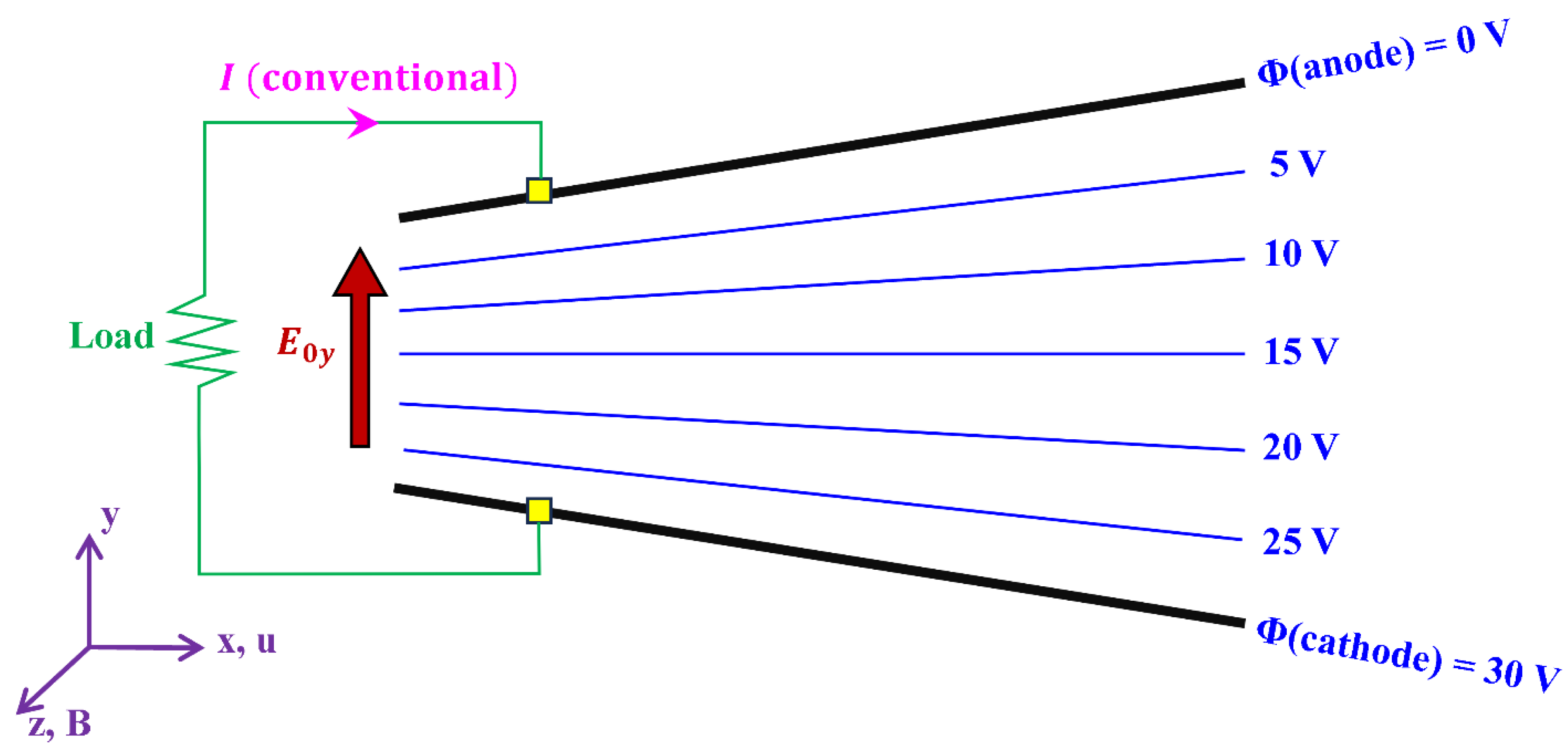
Figure 2.
Graphical illustration of a continuous-electrode Faraday channel, with a demonstration of the direction of the current density and the load electric field.
Figure 2.
Graphical illustration of a continuous-electrode Faraday channel, with a demonstration of the direction of the current density and the load electric field.
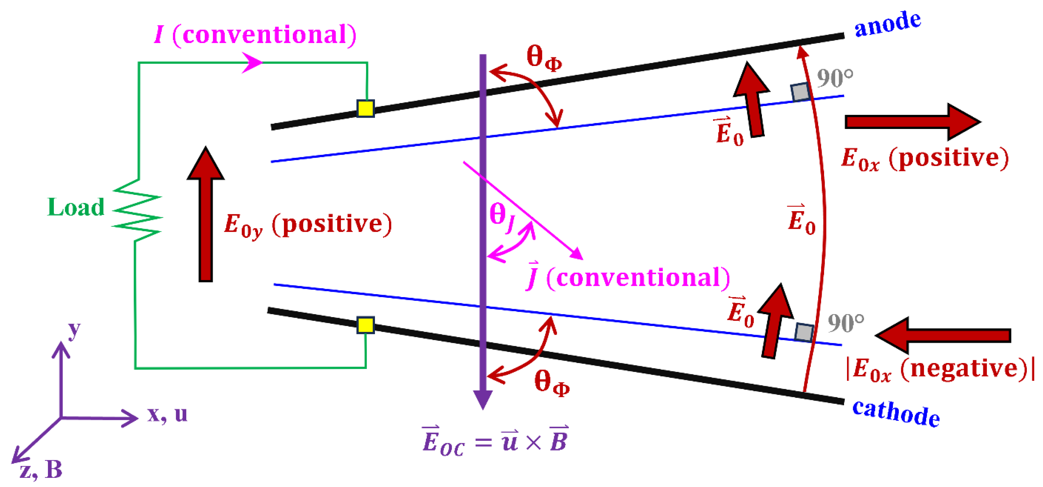
Figure 3.
Graphical illustration of a linear Hall channel, with a demonstration of the direction of the current density and the load electric field.
Figure 3.
Graphical illustration of a linear Hall channel, with a demonstration of the direction of the current density and the load electric field.
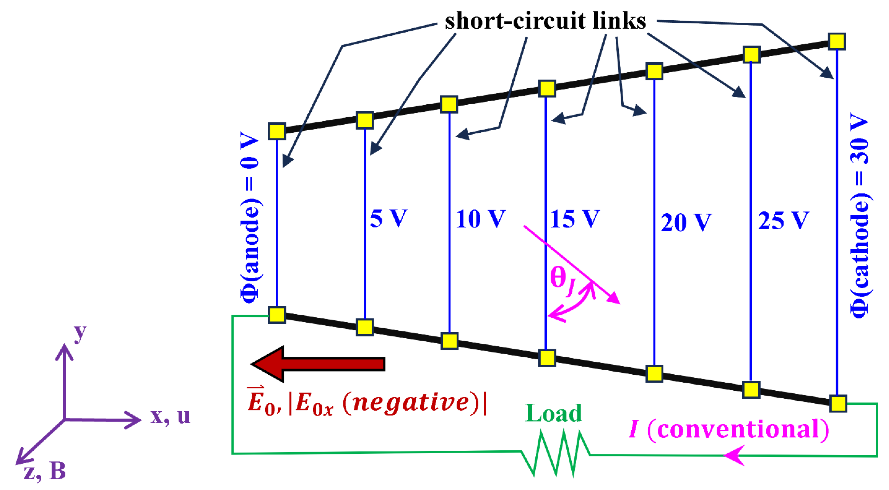
Figure 4.
Graphical illustration of a linear Hall channel, in the case of three external loads being powered simultaneously.
Figure 4.
Graphical illustration of a linear Hall channel, in the case of three external loads being powered simultaneously.
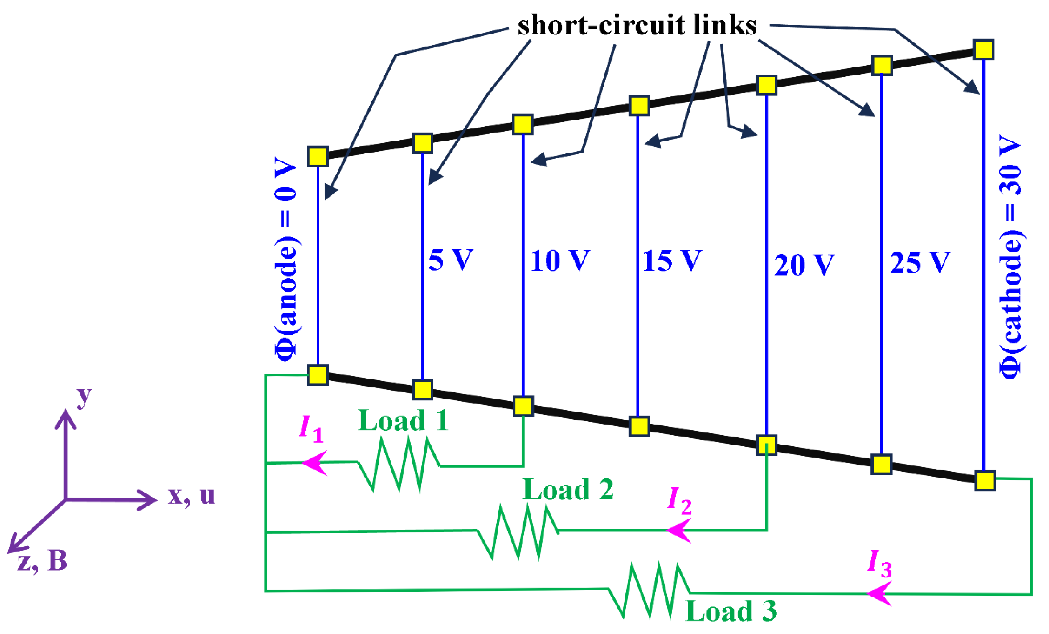
Figure 5.
Graphical illustration of a segmented-electrode Faraday channel, with a demonstration of the direction of the current density and the load electric field.
Figure 5.
Graphical illustration of a segmented-electrode Faraday channel, with a demonstration of the direction of the current density and the load electric field.
Figure 6.
Graphical illustration of a segmented-electrode Faraday channel, with a demonstration of the direction of the current density and the load electric field.
Figure 6.
Graphical illustration of a segmented-electrode Faraday channel, with a demonstration of the direction of the current density and the load electric field.
Figure 7.
Graphical illustration of a diagonal-electrode channel, with a demonstration of the direction of the current density and the load electric field.
Figure 7.
Graphical illustration of a diagonal-electrode channel, with a demonstration of the direction of the current density and the load electric field.
Figure 8.
Graphical illustration of a diagonal-electrode channel, in the case of three external loads being powered simultaneously.
Figure 8.
Graphical illustration of a diagonal-electrode channel, in the case of three external loads being powered simultaneously.

Table 1.
Gain in the power output for the linear Hall channel compared to the continuous-electrode Faraday channel at different Hall parameters.
Table 1.
Gain in the power output for the linear Hall channel compared to the continuous-electrode Faraday channel at different Hall parameters.
| Hall Parameter | Power Penalty Factor | ||
|---|---|---|---|
| Continuous-electrode Faraday | Linear Hall | ||
| 0 | 100% | 0% | 0 |
| 0.25 | 94.1176% | 5.8824 | 0.0625 |
| 0.5 | 80% | 20% | 0.25 |
| 0.75 | 64% | 36% | 0.5625 |
| 1 | 50% | 50% | 1 |
| 1.25 | 39.0244% | 60.9756% | 1.5625 |
| 1.5 | 30.7692% | 69.2308% | 2.25 |
| 1.75 | 24.6154% | 75.3846% | 3.0625 |
| 2 | 20% | 80% | 4 |
| 2.5 | 13.793% | 86.2069% | 6.25 |
| 3 | 10% | 90% | 9 |
| 4 | 5.8824% | 94.1176% | 16 |
| 5 | 3.8462% | 96.1538% | 25 |
| 6 | 2.7027% | 97.2973% | 36 |
| 7 | 2% | 98% | 49 |
| 8 | 1.5385% | 98.4615% | 64 |
| 9 | 1.2195% | 98.7805% | 81 |
| 10 | 0.9901% | 99.0099% | 100 |
Table 2.
Comparison between two types of linear magnetohydrodynamic channels.
| Quantity | Continuous-electrode Faraday | Linear Hall |
|---|---|---|
| 0 | ||
| 0 | ||
| P | ||
| Number of loads | 1 | 1 or more |
Table 3.
Comparison between the other two types of linear magnetohydrodynamic channels.
| Quantity | Segmented-electrode Faraday | Diagonal-electrode |
|---|---|---|
| Same as segmented-electrode Faraday | ||
| Same as segmented-electrode Faraday | ||
| Same as segmented-electrode Faraday | ||
| Same as segmented-electrode Faraday | ||
| Same as segmented-electrode Faraday | ||
| Same as segmented-electrode Faraday | ||
| P | Same as segmented-electrode Faraday | |
| Same as segmented-electrode Faraday | ||
| Same as segmented-electrode Faraday | ||
| Number of loads | multiple | 1 or more |
Disclaimer/Publisher’s Note: The statements, opinions and data contained in all publications are solely those of the individual author(s) and contributor(s) and not of MDPI and/or the editor(s). MDPI and/or the editor(s) disclaim responsibility for any injury to people or property resulting from any ideas, methods, instructions or products referred to in the content. |
© 2025 by the authors. Licensee MDPI, Basel, Switzerland. This article is an open access article distributed under the terms and conditions of the Creative Commons Attribution (CC BY) license (http://creativecommons.org/licenses/by/4.0/).
Copyright: This open access article is published under a Creative Commons CC BY 4.0 license, which permit the free download, distribution, and reuse, provided that the author and preprint are cited in any reuse.


