Submitted:
24 May 2025
Posted:
26 May 2025
You are already at the latest version
Abstract
Scoring functions are key elements in docking protocols as they approximate the binding affinity of a ligand (usually a small bioactive molecule) through calculating its interaction energy with a biomacromolecule (usually protein). In this study we present a pairwise comparison of scoring functions applying a multi-criterion decision-making approach based on InterCriteria analysis (ICrA). As criteria, the five scoring functions implemented in MOE (Molecular Operating Environment) software were selected and their performance on a set of protein-ligand complexes from the PDBbind database were compared. The following docking outputs were used: the best docking score; the lowest root-mean-square deviation (RMSD) between the predicted pose and the co-crystalized ligand; the RMSD between the best docking score pose and the co-crystalized ligand; the docking score of the pose with the lowest RMSD to the co-crystalized ligand. The impact of ICrA thresholds on the relations between the scoring functions was investigated. A correlation analysis was also performed and juxtaposed to ICrA. Our results reveal the lowest RMSD as the best performing docking output and two scoring functions (Alpha HB and London dG) as having the highest comparability. The proposed approach can be applied to any other scoring functions and protein-ligand complexes of interest.
Keywords:
molecular operating environment
; scoring functions
; molecular docking
; interCriteria analysis
1. Introduction
The search for hit compounds with specific biological activity requires considerable efforts and resources. The primary efforts concern the synthesis and biological testing of large number of compounds. This defines the strong interest of R&D pharmaceutical sector to computer-aided methods that facilitate rational drug design [1]. Among these methods, the molecular docking is particularly important when the structure of a biomacromolecule is resolved. The latter is used to predict the binding affinity of a ligand in the active site (by calculating docking scores employing scoring functions) based on the ligand docking poses (conformations and positions) in the binding site. Docking is also applied in virtual screening to identify active ligands for a specific macromolecular target among thousands to millions of compounds. In addition, the calculations of the docking scores are time-consuming, thus the selection of appropriate scoring functions could impact the whole computational procedure. Over the past decades, a number of studies have conducted comparative assessments of scoring functions implemented in both free and commercial docking software programs [2,3,4,5]. To evaluate the predictive power and examine the strengths and limitations of the scoring functions, several benchmark test sets have been developed [3,6,7]. These datasets are highly diverse, encompassing a wide range of protein families, ligand chemotypes, and binding affinities [8] thus providing good opportunities for comparison of docking scoring functions. Despite the studies [2,3,4,5] aiming at assessing and comparison of scoring functions in docking, the question about which scoring functions are more appropriate compared to others, remains open.
In this study the docking scoring functions implemented in the widely used drug discovery software platform Molecular Operating Environment (MOE, https://www.chemcomp.com/) [9], have been selected for comparison. MOE docking module operates with five scoring functions, namely London dG, ASE, Affinity dG, Alpha HB and GBVI/WSA dG [8,9]. The first four of them are empirical, while GBVI/WSA dG is a force-field one [5]. Empirical functions evaluate the binding affinity of protein-ligand complexes based on a set of weights defined by a multiple linear regression to experimentally measured affinities. The equation terms describe important enthalpic contributions like hydrogen bonding, ionic and hydrophobic interactions, as well as entropic contributions like loss in the ligand flexibility, etc. On the other hand, force-field based scoring functions use classical force fields to evaluate protein-ligand interactions and, in their simplest form, Lenard-Jones and Coulomb potentials are applied to describe the enthalpy terms.
The comparison of MOE scoring functions is based on the Comparative Assessment of Scoring Functions benchmark subset (CASF-2013) [3] of PDBbind database [6], which is a comprehensive collection of 195 protein-ligand complexes with available binding affinity data. CASF-2013 dataset has been used for assessment of scoring functions implemented in free software docking programs, such as AutoDock and Vina [10]. In [11], CASF-2013 dataset supported the evaluation of 12 scoring functions based on machine learning techniques. High-quality set of 195 test complexes enabled comparison and assessment of scoring functions embedded in some of the leading software platforms, like Schroedinger, MOE, Discovery Studio, SYBYL and GOLD [12]. CASF-2013, along with another independent benchmark dataset Community Structure-Activity Resource (CSAR 2014), have been used in an evaluation analysis of an improved version of the scoring function SPecificity and Affinity (SPA) [7]. CASF-2013 has also been applied to validate 3D convolution neural network (3D-CNN) scoring function and end-to-end 3D-CNN with mechanism for spatial attention [13,14], as well as the extensive validation of the scoring power of geometric graph learning with extended atom-types features for protein-ligand binding affinity prediction [15]. Thus, CASF-2013 has been selected as dataset in our study.
The InterCriteria analysis (ICrA) approach [16] has been applied for pairwise performance comparison of MOE scoring functions on CASF-2013. The expectations are ICrA to reveal any relations between the scoring functions by analyzing a variety of data outputs extracted from molecular docking. ICrA has been elaborated as a multi-criterion decision-making approach to detect possible relations between pairs of criteria when multiple objects are considered. Over the past years of research, the approach has already demonstrated evidence of its potential, when applied to economic, biomedical, pharmaceutical, industrial, and various other data sets and problem formulations [17]. One of the research objectives is to specify the general framework of the problems best addressable by the approach, as well as the connections between the new approach and the multi-criteria decision-making methods and types of correlation analyses [https://intercriteria.net]. Some case studies of the ICrA applications are freely accessible [https://intercriteria.net/studies/], e.g., over the world economic forum’s global competitiveness reports, genetic algorithms performance, ant colony optimization performance, and analysis of calorimetric data of blood serum proteome.
Recently, ICrA approach has been applied in the field of computer-aided drug design and computational toxicology in comparative studies of various scoring functions [18,19], as well as in in silico studies of biologically active molecules [20]. In contrast to our previous studies, here we apply ICrA on the CASF-2013 benchmark subset of PDBbind database covering several important docking outputs and investigating simultaneously how the variations of key ICrA thresholds could impact the comparison. A correlation analysis has also been performed and juxtaposed to the ICrA results. Our results outline what are the scoring functions that are the most and the least similar in-between and what docking outputs are the most comparable between the studied scoring functions. In addition, they demonstrate the applicability of ICrA to reveal new relations between the studied criteria.
2. Results and Discussion
For the CASF-2013 dataset, re-docking of the ligands in the protein-ligand complexes has been performed. The following data have been extracted from the 30 poses saved:
- i)
- the best docking score (the lower the better) – hereinafter referred to as BestDS;
- ii)
- the lowest root-mean-square deviation (RMSD) between the predicted pose and the ligand in the co-crystalized complex – hereinafter referred to as BestRMSD;
- iii)
- RMSD between the pose with the best docking score and the ligand in the co-crystalized complex – hereinafter referred to as RMSD_BestDS;
- iv)
- the docking score of the pose with the lowest RMSD to the ligand in the co-crystalized complex – hereinafter referred to as DS_BestRMSD.
For the sake of completeness, we have also investigated the possible relations to the experimental data available in CASF-2013. Based on the availability, Kd or Ki, expressed as (-logKd) or (-logKi), respectively, are used.
The collected information has been formatted for subsequent application of ICrA. All spreadsheets have been constructed in an identical way: the ligands from protein-ligand complexes have been considered as objects of research in terms of ICrA, while the different scoring functions (represented by BestDS, BestRMSD, RMSD_BestDS, or DS_BestRMSD), along with the binding affinity data, have been considered as criteria.
ICrA has been applied in two steps. Initially, it has been implemented on the data outputs extracted from molecular docking results as described above, with the conditionally defined in ICrAData values α = 0.75 and β = 0.25, based on which the ranges of consonance and dissonance are defined [21].
Table 1 summarizes the results obtained for the degrees of agreement µ between the five scoring functions of MOE and the binding affinity data of the studied complexes, after the ICrA application for all aforementioned docking outputs. Colors in Table 1 reproduce the ones used in ICrAData, as explained above, for the conditionally defined in ICrAData values α = 0.75 and β = 0.25.
As seen from Table 1, “varicolored” ICrA results have been obtained only when BestRMSD is considered. For the rest docking outputs ICrA does not outline any significant relations (other than in dissonance) between the five investigated scoring functions in MOE, as well as between the scoring functions and the binding affinity data – all hit the dissonance zone only (colored in magenta).
In the second step, the impact of the variations in the α and β values on the investigated relations has been explored. As mentioned above, the thresholds α and β might be determined algorithmically, or chosen by the user. Since these parameters define the thresholds for positive consonance/dissonance/negative consonance between the studied pairs of criteria, we investigated how their values could impact the relations between the scoring functions. We varied the difference between α and β (keeping their sum to 1.00) starting from 0.5 (α = 0.75 and β = 0.25) and decreasing it gradually to 0.2 (α = 0.6 and β = 0.4) to follow how these values affect the relations between the investigated scoring functions (for clarity, these analyses are reported using ICrA colors in supplementary tables S1-S5). The results are summarized in Table 2 and Table 3, based on the following two indicators: the number of pairs in positive consonance for each docking output (Table 2), and the number of docking outputs for each pair of scoring functions in positive consonance (Table 3).
The first indicator, number of pairs in positive consonance, could be considered as a measure for “sensitivity” of the corresponding docking output to the α and β values. The second one, number of docking outputs for each pair in positive consonance, allows to compare the scoring functions based on the number of the docking outputs – the more the docking outputs in positive consonance, the more similar is the performance of the studied pairs of scoring functions.
As expected, the decrease in the difference between α and β results in a higher number of pairs in positive consonance thus raising the question what are the most appropriate α and β values. The values of 0.67/0.33 and 0.65/0.35 show almost identical results, and the 0.67/0.33 appears a good compromise between “no” and “many” pairs in positive consonance allowing simultaneously certain tolerance in comparability between the studied criteria.
In addition, the values α = 0.67 and β = 0.33 allow the authors to present an alternative scale for consonance/dissonance. If the scale of consonance/dissonance outlined in Atanassov et al. [21], might be considered as a scale of “quarters”, here а kind of scale of “thirds” is intentionally considered, corresponding to α = 0.67 (approximately two-thirds) and β = 0.33 (approximately one-third). For better understanding, Figure 1 represents the respective interpretative intuitionistic triangle.
In this case, the pair of criteria are said to be in:
- positive consonance, whenever ≥ 2/3 and < 1/3;
- negative consonance, whenever < 1/3 and ≥ 2/3;
- dissonance, whenever 0 ≤ < 2/3, 0 ≤ < 2/3 and 2/3 ≤ + ≤ 1; and
- uncertainty, 0 ≤ < 2/3, 0 ≤ < 2/3 and 0 ≤ + < 2/3.
As seen from Figure 1, the presented scale of “thirds” preserves the symmetry in the interpretative intuitionistic triangle, in accordance with the original “quarters”-based symmetry [21]. Thus, the combination α = 0.67 and β = 0.33 appears an appropriate selection in this investigation.
According to the pairwise performance comparison of the MOE scoring functions (Table 3), the most persistent results are:
- 1)
- the absence of any kind of agreement in all explored values of α and β with the experimental data (except one, between GBVI/WSA dG - (-logKd) or (-logKi) at α = 0.60 and β = 0.40, rows highlighted in grey in Table 3). Such result is in accordance with our previous studies [19]. The lack of any agreement might be explained also with the fact that even implementing a variety of scoring terms and becoming more sophisticated, the scoring functions are still a computational approximation aiming to assist mostly in prediction of ligand binding poses as confirmed by the results with BestRMSD docking output (Table 2).
- 2)
- positive consonance between two scoring functions – Alpha HB and London dG: in particular, for 0.67/0.33 thresholds values they are comparable in all four docking outputs (a row in bold in Table 3). The result suggests that these scoring functions might be used interchangeably. At the same time some pairs show small comparability (Affinity dG - London dG and GBVI/WSA dG - London dG) suggesting that they can complement each other in consensus docking studies.
Figure 2 and Figure 3 demonstrate the results from ICrA implementation for the explored values of thresholds α and β, respectively for BestDS and RMSD_BestDS. Both figures show the ICrA screenshots at conditionally defined thresholds values α = 0.75 and β = 0.25 (subplot a), α = 0.70 and β = 0.30 (subplot b), α = 0.67 and β = 0.33 (subplot c), α = 0.65 and β = 0.35 (subplot d), and α = 0.60 and β = 0.40 (subplot e).
As seen from Figure 2, applying new values of thresholds leads to appearance of pairs in positive consonance. For α = 0.70 and β = 0.30 (Figure 2b) and α = 0.67 and β = 0.33 (Figure 2c), positive consonance appears between the scoring functions Alpha HB - London dG, toward no identified significant relations with the conditionally defined thresholds values (Figure 2a). Further decreasing the difference between α and β leads to one more pair in positive consonance – Alpha HB - ASE for α = 0.65 and β = 0.35 (Figure 2d), and additionally 3 more pairs in positive consonance – namely Affinity dG - Alpha HB, Affinity dG - ASE, and ASE - London dG at α = 0.60 and β = 0.40 (Figure 2e).
As seen from Figure 3 and Table 1 as well, RMSD_BestDS is the docking output with the highest number of newly appeared significant relations when the new values of the thresholds are applied. Altogether 5 pairs of scoring functions show positive consonance, namely: Affinity dG - Alpha HB, Affinity dG - ASE, Affinity dG - GBVI/WSA dG, Alpha HB - GBVI/WSA dG, and Alpha HB - London dG at α = 0.67 and β = 0.33 (Figure 3c) in comparison to no significant relations identified at the conditionally defined thresholds values (Figure 3a) and α = 0.70 and β = 0.30 (Figure 3b). Further decreasing of the difference between α and β leads to two more pairs in positive consonance – between ASE - GBVI/WSA dG and ASE - London dG at α = 0.65 and β = 0.35 (Figure 3d), and even to 3 additional ones – between Affinity dG - London dG, Alpha HB - ASE, and GBVI/WSA dG - London dG at α = 0.60 and β = 0.40 (Figure 3e).
As mentioned above, the most “varicolored” picture from ICrA implementation is when the BestRMSD is considered (results not shown as a figure). As seen from Table 1, positive consonance has been observed for almost all pairs of scoring functions, while the other two pairs of scoring functions – ASE - GBVI/WSA dG and GBVI/WSA dG - London dG, are very close to the conditionally defined thresholds values α = 0.75 and β = 0.25. Then, still at the thresholds values α = 0.70 and β = 0.30, all pairs of scoring functions become in positive consonance. Based on this analysis, one may conclude that according to the BestRMSD, all scoring functions give quite similar results.
For the DS_BestRMSD output, only one pair of scoring functions – Alpha HB - London dG falls into the interval of positive consonance (Table 1, results not shown as a figure) when applying values of thresholds α = 0.70 and β = 0.30. Further decrease in the difference between α and β leads to three more pairs in positive consonance – between Affinity dG - GBVI/WSA dG, Alpha HB - ASE, and ASE - London dG, only at α = 0.60 and β = 0.40.
For the completeness of the comparison of the five scoring functions, a correlation analysis (CA) has also been performed. Table 4 summarizes the results obtained by ICrA and CA for all docking outputs. CA shows higher correlation only for BestRMSD, while for the other docking outputs the observed correlations are relatively low. In case of BestRMSD, the highest correlation coefficients somehow coincide with the highest values of ICrA degrees of agreement. In particular, the relation between Alpha HB and London dG is evaluated with the highest values of degree of agreement by ICrA and with the second-best correlation coefficient by CA. Figure 4 illustrates the correlation in terms of CA between Alpha HB and London dG for BestRMSD.
The absence of correlation, estimated by the Pearson correlation coefficients, between the docking scores and the experimental data on binding affinity of the ligands in the studied complexes is not surprising. This result could not be related only to the heterogeneity of the experimental data (different measures of affinity, different methods and experimental protocols, various protein-ligand complexes) in the used dataset, but rather to the fact that molecular docking has not initially been designed for the purpose of correlation of docking scores with experimental binding affinities [22]. Absence of such correlations has also been confirmed in our previous studies employing much more consistent experimental data on binding affinities of a homologous series of 88 benzamidine type ligands toward thrombin, trypsin, and factor Xa [19].
As seen from Table 4 and Figure 4, ICrA may offer enhanced capabilities over CA by enabling the identification of additional relationships among the evaluated scoring functions. This might be explained by the fact that ICrA, as well as CA, reports the degree of coincidence – in terms of ICrA, this is positive consonance. Both CA and ICrA report the negative correlation (negative consonance in terms of ICrA), in which the values for one criterion increase while at the same time the values of the other criterion decrease. Unlike CA, ICrA also allows for classifying the criteria relations in dissonance, as well as accounting of the degree of uncertainty, which makes the advantage of ICrA over CA.
3. Materials and Methods
3.1. Dataset
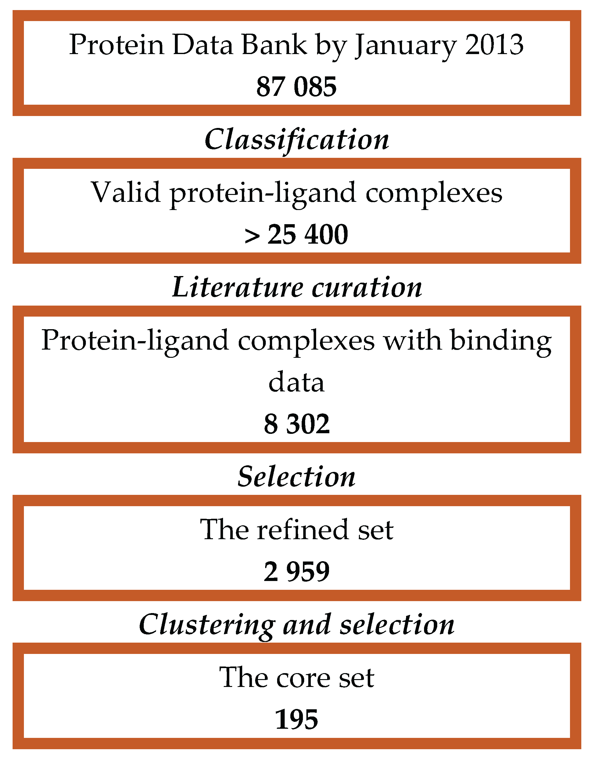
In the current investigation, CASF-2013 has been selected considering the quality of complex structures and binding data in accordance with [3] (Figure 5).
The final CASF-2013 dataset consists of 195 protein-ligand complexes with collected binding affinity data selected out of 8302 protein-ligand complexes recorded in the PDBbind database (v. 2013). The qualified complexes have been classified in 65 clusters by 90% similarity in protein sequences. Three representative complexes are chosen from each cluster to control sample redundancy.
3.2. Molecular Docking
MOE v. 2022 has been used for molecular docking studies. Prior to re-docking, all 195 protein-ligand complexes have been protonated using the Protonate3D tool in MOE. The tool assigns hydrogens to structures following the optimal free energy proton geometry and the ionization states of titratable protein groups. The rigid protein/flexible ligand has been used. The active site has been defined by ligand atoms and the water molecules have been removed from the binding sites of the studied proteins. The placement was done by a triangle matcher algorithm.
Re-docking of the ligands in the protein-ligand complexes has been performed, applying all available scoring functions in MOE v. 2022, namely London dG, ASE, Affinity dG, Alpha HB and GBVI/WSA dG, briefly described below [8,9]:
- ASE is based on the Gaussian approximation and depends on the radii of the atoms and the distance between the ligand atom – receptor atom pairs. ASE is proportional to the sum of the Gaussians over all ligand atom-receptor atom pairs.
- Affinity dG is a linear function that calculates the enthalpy contribution to the binding free energy, including terms based on: interactions between H-bond donor-acceptor pairs, ionic interactions, metal ligation, hydrophobic interactions, also unfavorable interactions (between hydrophobic and polar atoms) and favorable interactions (between any two atoms).
- Alpha HB is a linear combination of two terms: (i) the geometric fit of the ligand to the binding site with regard to the attraction and repulsion depending on the distance between the atoms; (ii) H-bonding effects.
- London dG estimates the free binding energy of the ligand, counting for the average gain or loss of rotational and translational entropy, the loss of flexibility of the ligand, the geometric imperfections of H-bonds and metal ligations compared to the ideal ones, and the desolvation energy of atoms.
- GBVI/WSA dG estimates the free energy of binding of the ligand considering the weighted terms for the Coulomb energy, solvation energy, and van der Waals contributions.
Up to 30 poses per ligand have been saved for each of the protein-ligand complexes and each one of the investigated scoring functions.
3.3. InterCriteria Analysis Approach
Developed in 2014 by Atanassov et al. [16], the ICrA approach is derived on the basis of two mathematical formalisms, i.e., index matrices (IM) [23] and intuitionistic fuzzy sets (IFS) [24]. Relying on IM and IFS, ICrA allows for identification of intercriteria relations in terms of consonance or dissonance, thus differentiating from the classical correlation analysis.
In the concept of IFS [17], Atanassov builds on Zadeh’s theory of fuzzy sets [25], which, on their side, are an extension of the classical notion of set. In the classical set theory, an element either belongs or does not belong to the set, therefore the membership of the element to the set is represented by the values 0 for non-membership, or 1 otherwise. The fuzzy set theory introduces a degree of membership μ of the element x to the set, such as μ ∈ [0; 1]. The theory of IFS further expands this notion by including the degree of non-membership ν of the element x to the set, such as ν ∈ [0; 1].
In mathematical terms, a set A is defined as an intuitionistic fuzzy set as:
where X is the universum, and the two mappings μA(x), νA(x): A → [0, 1] are respectively the degree of membership and the degree of non-membership of each element x ∈ X, such as 0 ≤ μA(x) + νA(x) ≤ 1. The boundary conditions are 0 and 1, both giving the classical set.
A = {〈x, μA(x), νA(x)〉 | x ∈ X},
The ICrA approach uses as input a two-dimensional IM. The 2D IM is represented by a set indexing the rows, a set indexing the columns, and a set of elements corresponding to each pair of row and column index. In the case of ICrA, the IM can be written as [O, C, eO,C], where O and C are respectively the set of row and column indexes and O stands for objects, while C stands for criteria, and eO,C corresponds to the evaluation of each object O against the criterion C. If we denote by m the number of objects, and by n the number of criteria, the input IM for ICrA can be represented as follows:
| C1 | … | Ck | … | Cn | |
| O1 | … | … | |||
| … | … | … | … | … | … |
| Oi | … | … | |||
| … | … | … | … | … | … |
| Om | … | … |
In the next step of ICrA, relations are formed between every two elements of the matrix, thus the criteria’s evaluations are compared in pairs for all objects in the matrix. Then each pair of relations and is assessed to determine whether both relations coincide, i.e., (, ∈ {<, =, >}), or are dual, i.e., is the relation of type “>”, while is relation of type “<” (or vice-versa). In the first case, the score of agreements (or similarities) is incremented, while in the second case the score of disagreements (dissimilarities) is incremented. In the remaining cases the score of uncertainty is incremented.
The total number of pairwise comparisons between the evaluations of m objects is m(m − 1)/2, therefore , where counts the number of the identical relations, while counts the number of dual relations.
For every k, l (1 ≤ k ≤ l ≤ m and m ≥ 2), two normalized values are obtained from the above counters:
- , called the degree of agreement in terms of ICrA, and
- , called the degree of disagreement in terms of ICrA.
The pair , constructed from these two numbers, plays the role of intuitionistic fuzzy evaluation of the relation between any two criteria Ck and Cl. The output IM puts together all those intuitionistic fuzzy pairs, as follows:
| C1 | … | Ck | … | Cn | |
| C1 | 〈1, 0〉 | … | … | ||
| … | … | … | … | … | … |
| Ck | … | 〈1, 0〉 | … | ||
| … | … | … | … | … | … |
| Cn | … | … | 〈1, 0〉 |
The thresholds for and are determined algorithmically or are indicated by the user. Let α, β ∈ [0, 1] (with α > β) be the thresholds values, then the pair of criteria Ck and Cl are said to be in:
- 3.
- positive consonance, whenever > α and < β;
- 4.
- negative consonance, whenever < β and > α;
- 5.
- dissonance, otherwise.
3.4. Software Implementation of ICrA
A software application that implements the ICrA algorithms, called ICrAData, v.2.5 has been used during the calculations. It is freely available from http://intercriteria.net/software/, along with the source code, a README file and proper examples. The ICrAData interface allows for: different variants of ICrA and different algorithms for intercriteria relations calculation to be chosen; input matrix to be read from a file or pasted from the clipboard; input matrix to be transposed according to the investigation aims; index matrices for the degrees of agreements and disagreements to be visualized according to the user’s needs; thresholds values for α and β to be defined by the user (conditionally defined in ICrAData as α = 0.75 and β = 0.25, as introduced in [21]); graphical interpretation of the results to be visualized by the intuitionistic fuzzy triangle, etc. For better visualization, the tables presenting index matrices for the degrees of agreements and disagreements use colors for the cells’ values: green to indicate positive consonance, red for negative consonance, and magenta for the cases of dissonance.
3.5. Correlation Analysis
The correlations between each two variables investigated in this study have been calculated in MS Excel using Pearson’s correlation coefficient (Pearson product moment correlation coefficient) [28].
4. Conclusions
Altogether five scoring functions available in MOE software package (London dG, Affinity dG, Alpha HB, ASE and GBVI/WSA dG) have been compared for their performance by four docking outputs (BestDS, BestRMSD, RMSD_BestDS, and DS_BestRMSD) on the benchmark subset CASF-2013 consisting of 195 protein-ligand complexes from PDBbind database.
The collected information has been subjected to ICrA using the ICrAData software, initially, with the conditionally defined values of thresholds determining the intervals of consonance and dissonance and subsequent investigation of the impact of the different thresholds values. It has been shown that at the conditionally defined thresholds (0.75/0.25) no relations between the scoring functions can be outlined for all considered data outputs from molecular docking, except BestRMSD. More “varicolored” relations between the scoring functions appear when the values of threshold determining the intervals of consonance and dissonance have gradually been changed towards their convergence. For the particular collection of scoring functions and dataset the optimal thresholds values of 0.67/0.33 have been determined for the intervals of positive consonance, dissonance and negative consonance, corresponding to the scale of “thirds”. The scoring functions Alpha HB and London dG have been outlined as a pair appearing in positive consonance in all investigated docking outputs suggesting that these scoring functions might be used interchangeably. Two other pairs of scoring functions (Affinity dG - London dG and GBVI/WSA dG - London dG) were mostly in dissonance (except in BestRMSD) suggesting that they can complement each other in consensus docking studies. In addition, the docking output BestRMSD was keeping in positive consonance all pairs of scoring functions thus confirming that the studied scoring functions perform best in reproducing the binding poses of the co-crystalized ligands. At the same time the comparison between the ICrA and CA results illustrates the advantage of ICrA over CA for identification of new relations between the investigated criteria.
To the best of our knowledge this is the first systematic investigation of ICrA to assess the pairwise performance comparison of scoring functions available in a molecular software package considering a variety of data outputs from molecular docking in various protein targets of pharmacological interest. The proposed approach can be applied to any other scoring functions and software packages as well as on any other datasets of protein-ligand complexes of research interest.
Supplementary Materials
The following supporting information can be downloaded at the website of this paper posted on Preprints.org
Author Contributions
Conceptualization, T.P., I.P. and K.A.; methodology, T.P., I.P. and K.A.; software, M.A., P.A., I.T., D.J., I.L. and T.P.; validation, M.A., P.A., I.T., I.L. and T.P..; formal analysis, M.A., P.A., I.T., D.J., I.L., K.A., I.P. and T.P.; investigation, M.A., P.A., I.T., D.J., I.L., K.A., I.P. and T.P.; resources, M.A., P.A., I.T., D.J. and I.L.; data curation, M.A., P.A., I.T., D.J. and I.L.; writing—original draft preparation, M.A., I.P. and T.P.; writing—review and editing, M.A., P.A., I.T., D.J., I.L., K.A., I.P. and T.P.; visualization, M.A., D.J., I.P. and T.P.; supervision, K.A., I.P. and T.P.; project administration, K.A., I.P. and T.P.; funding acquisition, I.T., K.A. and T.P. All authors have read and agreed to the published version of the manuscript.
Funding
K.A. and T.P. gratefully acknowledge the funding by the Bulgarian National Science Fund under the grant KP-06-N72/8 from 14.12.2023 “Intuitionistic Fuzzy Methods for Data Analysis with an Emphasis on the Blood Donation System in Bulgaria”, while M.A., P.A., I.T., D.J., I.L., T.P. – the grant KP-06-COST/3 from 23 May 2023 with regard to COST Action CA21145 “European Network for Diagnosis and Treatment of Antibiotic-resistant Bacterial Infections (EURESTOP)”.
Data Availability Statement
The original contributions presented in the study are included in the article and supplementary material. Further inquiries can be directed to the corresponding author.
Acknowledgments
K.A. and T.P. gratefully acknowledge the funding by the Bulgarian National Science Fund under the grant KP-06-N72/8 from 14.12.2023 “Intuitionistic Fuzzy Methods for Data Analysis with an Emphasis on the Blood Donation System in Bulgaria”, while M.A., P.A., I.T., D.J., I.L., T.P. – the grant KP-06-COST/3 from 23 May 2023 with regard to COST Action CA21145 “European Network for Diagnosis and Treatment of Antibiotic-resistant Bacterial Infections (EURESTOP)”.
Conflicts of Interest
The authors declare no conflicts of interest.
References
- Höltje, H.-D.; Sippl, W.; Rognan, D.; Folkers, G. Molecular Modeling: Basic Principles and Applications, 3rd rev. expanded ed.; Wiley-VCH: Weinheim, Germany, 2008. [Google Scholar]
- Cheng, T.; Li, X.; Li, Y.; Liu, Z.; Wang, R. Comparative Assessment of Scoring Functions on a Diverse Test Set. J. Chem. Inf. Model. 2009, 49, 1079–1093. [Google Scholar] [CrossRef] [PubMed]
- Li, Y.; Liu, Z. H.; Han, L.; Li, J.; Liu, J.; Zhao, Z. X.; Li, C. K.; Wang, R. X. Comparative Assessment of Scoring Functions on an Updated Benchmark: I. Compilation of the Test Set. Journal of Chemical Information Modeling 2014, 54, 1717–1736. [Google Scholar] [CrossRef] [PubMed]
- Xu, W.; Lucke, A. J.; Fairlie, D. P. Comparing Sixteen Scoring Functions for Predicting Biological Activities of Ligands for Protein Targets. Journal of Molecular Graphics and Modelling 2015, 57, 76–88. [Google Scholar] [CrossRef]
- Su, M.; Yang, Q.; Du, Y.; Feng, G.; Liu, Z.; Li, Y.; Wang, R. Comparative Assessment of Scoring Functions: The CASF-2016 Update. J. Chem. Inf. Model. 2019, 59, 895–913. [Google Scholar] [CrossRef]
- Wang, R.; Fang, X.; Lu, Y.; Wang, S. The PDBbind Database: Collection of Binding Affinities for Protein-Ligand Complexes with Known Three-Dimensional Structures. Journal of Medical Chemistry 2004, 47, 2977–2980. [Google Scholar] [CrossRef]
- Yan, Z.; Wang, J. Incorporating specificity into optimization: evaluation of SPA using CSAR 2014 and CASF 2013 benchmarks. J Comput Aided Mol Des. 2016, 30, 219–227. [Google Scholar] [CrossRef] [PubMed]
- Kalinowsky, L.; Weber, J.; Balasupramaniam, S.; Baumann, K.; Proschak, E. A Diverse Benchmark Based on 3D Matched Molecular Pairs for Validating Scoring Functions. ACS Omega 2018, 3, 5704–5714. [Google Scholar] [CrossRef] [PubMed]
- Molecular Operating Environment, The Chemical Computing Group, v. 2016.08, http://www.chemcomp.com.
- Gaillard, T. Evaluation of AutoDock and AutoDock Vina on the CASF-2013 Benchmark. J Chem Inf Model. 2018, 58, 1697–1706. [Google Scholar] [CrossRef] [PubMed]
- Khamis, M. A.; Gomaa, W. Comparative assessment of machine-learning scoring functions on PDBbind 2013. Engineering Applications of Artificial Intelligence 2015, 45, 136–151. [Google Scholar] [CrossRef]
- Li, Y.; Su, M.; Liu, Z.; Li, J.; Liu, J.; Han, L.; Wang, R. Assessing protein-ligand interaction scoring functions with the CASF-2013 benchmark. Nat Protoc. 2018, 13, 666–680. [Google Scholar] [CrossRef] [PubMed]
- Wang, Y.; Qiu, Z.; Jiao, Q.; Chen, C.; Meng, Z.; Cui, X. Structure-based Protein-drug Affinity Prediction with Spatial Attention Mechanisms. In Proceedings of the 2021 IEEE International Conference on Bioinformatics and Biomedicine (BIBM), Houston, TX, USA, 9-12 December 2021; pp. 92–97. [Google Scholar]
- Wang, Y.; Wei, Z.; Xi, L. Sfcnn: a novel scoring function based on 3D convolutional neural network for accurate and stable protein-ligand affinity prediction. BMC Bioinformatics 2022, 23, 222. [Google Scholar] [CrossRef] [PubMed]
- Rana, M. M.; Nguyen, D. D. Geometric graph learning with extended atom-types features for protein-ligand binding affinity prediction. Computers in Biology and Medicine 2023, 164, 107250. [Google Scholar] [CrossRef] [PubMed]
- Atanassov, K.; Mavrov, D.; Atanassova, V. Intercriteria Decision making: a new approach for multicriteria decision making, based on index matrices and intuitionistic fuzzy sets. Issues IFSs and GNs 2014, 11, 1–8. [Google Scholar]
- Chorukova, E.; Marinov, P.; Umlenski, I. , ; Atanassov, K. Ed.; Springer: Cham, Switzerland, 2021; Vol. 934, pp. 453-469.Approach. In Research in Computer Science in the Bulgarian Academy of Sciences. Studies in Computational Intelligence, 1st ed.; Atanassov, K., Ed.; Springer: Cham, Switzerland, 2021; Vol. 934, pp. 453–469. [Google Scholar]
- Jereva, D.; Angelova, M.; Tsakovska, I.; Alov, P.; Pajeva, I.; Miteva, M.; Pencheva, T. InterCriteria Analysis Approach for Decision-making in Virtual Screening: Comparative Study of Various Scoring Functions. Lecture Notes in Networks and Systems 2022, 374, 67–78. [Google Scholar]
- Jereva, D.; Pencheva, T.; Tsakovska, I.; Alov, P.; Pajeva, I. Exploring Applicability of InterCriteria Analysis to Evaluate the Performance of MOE and GOLD Scoring Functions. Studies in Computational Intelligence 2021, 961, 198–208. [Google Scholar]
- Tsakovska, I.; Alov, P.; Ikonomov, N.; Atanassova, V.; Vassilev, P.; Roeva, O. , Jereva, D.; Atanassov, K.; Pajeva, I.; Pencheva, T. Intercriteria analysis implementation for exploration of the performance of various docking scoring functions. Studies in Computational Intelligence 2021, 902, 88–98. [Google Scholar]
- Atanassov, K.; Atanassova, V.; Gluhchev, G. Intercriteria analysis: ideas and problems. Notes Intuit. Fuzzy Sets 2015, 21, 81–88. [Google Scholar]
- Medina-Franco, J. L. Grand Challenges of Computer-Aided Drug Design: The Road Ahead. Front. Drug Discov. 2021, 1, 728551. [Google Scholar] [CrossRef]
- Atanassov, K. Index Matrices: Towards an Augmented Matrix Calculus, Studies in Computational Intelligence, 1st ed.; Springer International Publishing: Cham, Switzerland, 2014. [Google Scholar]
- Atanassov, K. Intuitionistic fuzzy logics, 1st ed.; Springer: Cham, Switzerland, 2017. [Google Scholar]
- Zadeh, L. A. Fuzzy Sets. Information and Control 1965, 8, 338–353. [Google Scholar] [CrossRef]
- Roeva, O.; Vassilev, P.; Angelova, M.; Su, J.; Pencheva, T. Comparison of Different Algorithms for InterCriteria Relations Calculation. In Proceedings of the IEEE 8th International Conference on Intelligent Systems, Sofia, Bulgaria, 4-6 September 2016; pp. 567–572. [Google Scholar]
- Roeva, O.; Vassilev, P.; Ikonomov, N.; Angelova, M.; Su, J.; Pencheva, T. On Different Algorithms for InterCriteria Relations Calculation. In Intuitionistic Fuzziness and Other Intelligent Theories and Their Applications. Studies in Computational Intelligence, 1st ed.; Hadjiski, M., Atanassov, K., Eds.; Springer: Cham, Switzerland, 2019. [Google Scholar]
- Correlation analysis. Available online: https://www.questionpro.com/features/correlation-analysis.html (accessed on 9 January 2025).
Figure 1.
Interpretative intuitionistic triangle in the case of “thirds”.
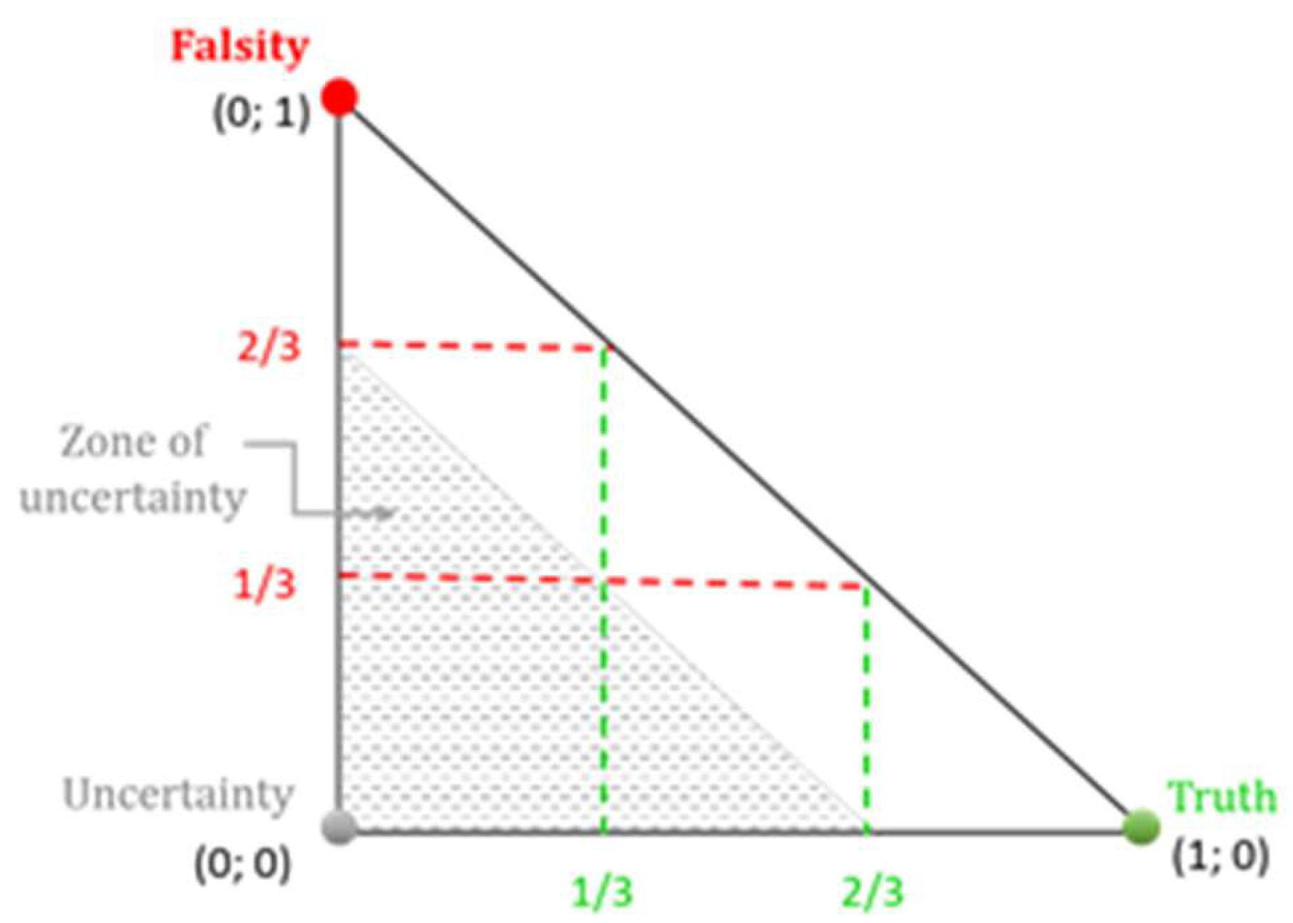
Figure 2.
ICrA implementation with different values of α and β thresholds to assess the scoring functions based on BestDS.
Figure 2.
ICrA implementation with different values of α and β thresholds to assess the scoring functions based on BestDS.
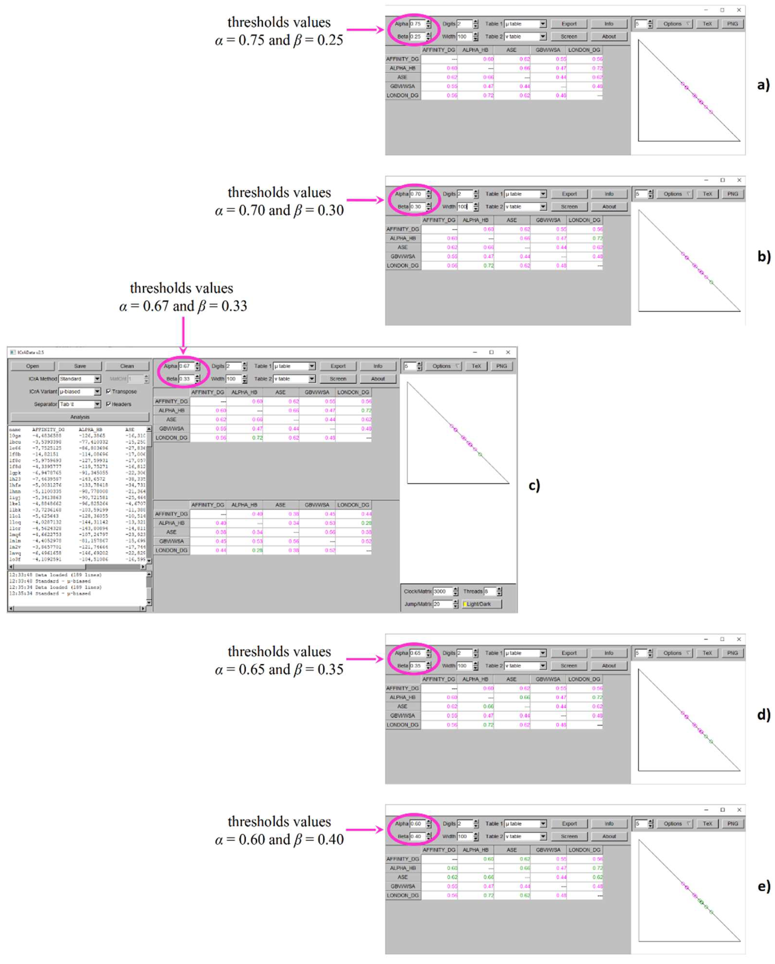
Figure 3.
ICrA implementation with different values of α and β thresholds to assess the five scoring functions based on RMSD_BestDS.
Figure 3.
ICrA implementation with different values of α and β thresholds to assess the five scoring functions based on RMSD_BestDS.
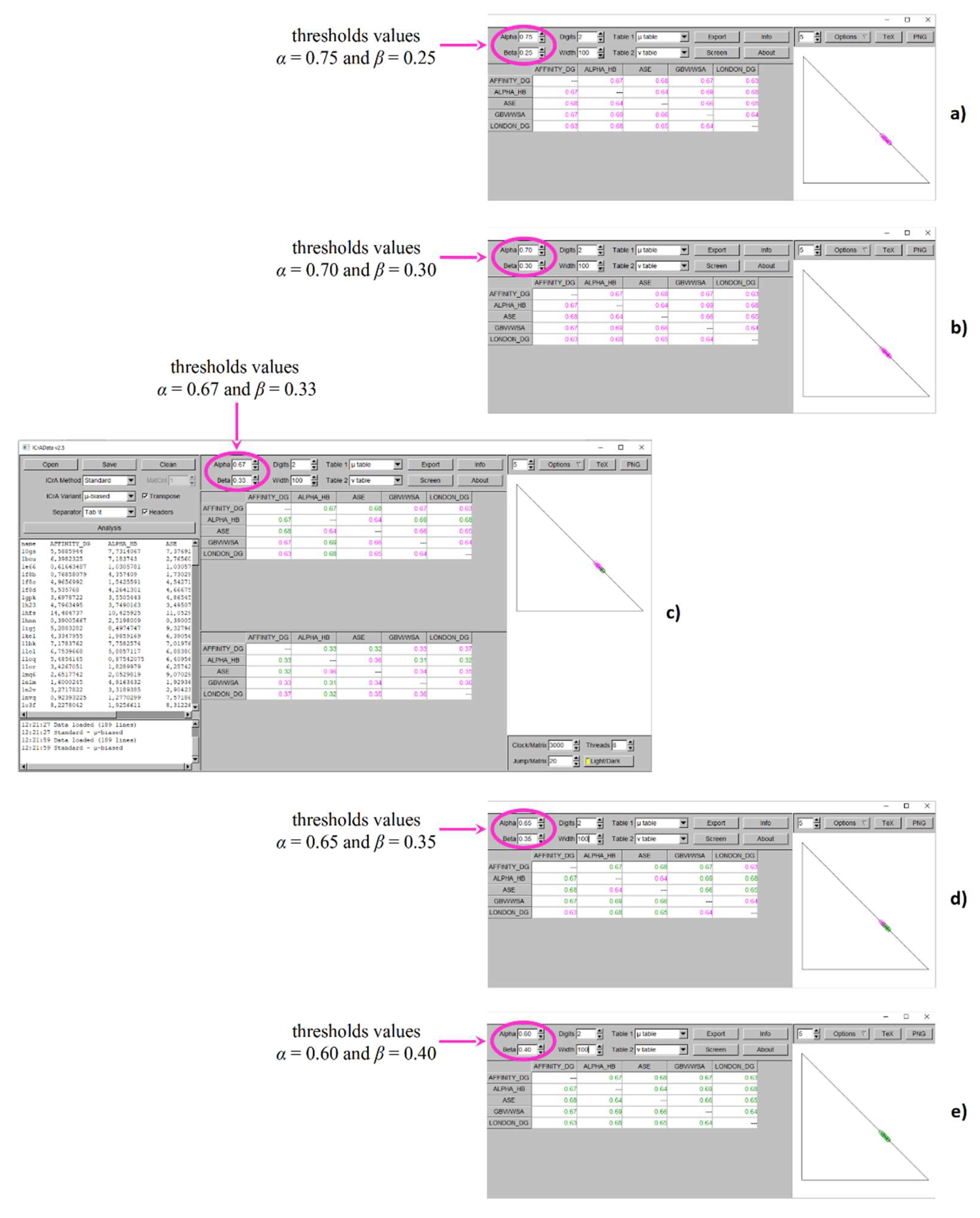
Figure 4.
Correlation analysis for Alpha HB and London dG based on the BestRMSD.
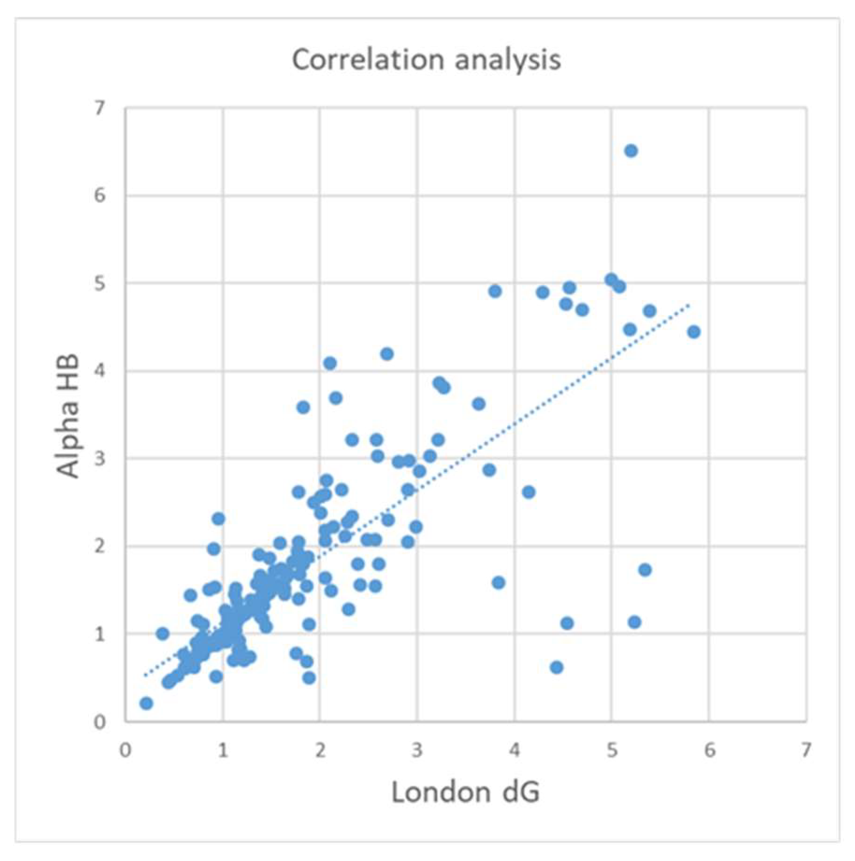
Figure 5.
CASF-2013 dataset selection (adapted from [3]).
Figure 5.
CASF-2013 dataset selection (adapted from [3]).
| BestDS | BestRMSD | RMSD_BestDS | DS_BestRMSD | |||||
|---|---|---|---|---|---|---|---|---|
| ICrA | CA | ICrA | CA | ICrA | CA | ICrA | CA | |
| Affinity dG - Alpha HB | 0.60 | 0.20 | 0.81 | 0.74 | 0.67 | 0.55 | 0.59 | 0.19 |
| Affinity dG - ASE | 0.62 | 0.23 | 0.77 | 0.68 | 0.68 | 0.53 | 0.57 | 0.03 |
| Affinity dG - GBVI/WSA dG | 0.55 | 0.12 | 0.83 | 0.81 | 0.67 | 0.55 | 0.61 | 0.22 |
| Affinity dG - London dG | 0.56 | 0.14 | 0.78 | 0.66 | 0.63 | 0.35 | 0.56 | 0.06 |
| Alpha HB - ASE | 0.66 | 0.54 | 0.79 | 0.77 | 0.64 | 0.45 | 0.62 | 0.42 |
| Alpha HB - GBVI/WSA dG | 0.47 | -0.10 | 0.76 | 0.63 | 0.69 | 0.53 | 0.45 | -0.05 |
| Alpha HB - London dG | 0.72 | 0.55 | 0.84 | 0.79 | 0.68 | 0.52 | 0.70 | 0.47 |
| ASE - GBVI/WSA dG | 0.44 | -0.19 | 0.73 | 0.57 | 0.66 | 0.48 | 0.36 | -0.16 |
| ASE - London dG | 0.62 | 0.29 | 0.77 | 0.68 | 0.65 | 0.42 | 0.60 | 0.24 |
| GBVI/WSA dG - London dG | 0.48 | -0.16 | 0.73 | 0.57 | 0.64 | 0.36 | 0.46 | -0.06 |
| Affinity dG - (-logKd) or (-logKi) | 0.45 | -0.08 | 0.57 | 0.21 | 0.50 | 0.19 | 0.53 | 0.06 |
| Alpha HB -(-logKd) or (-logKi) | 0.40 | -0.29 | 0.53 | 0.10 | 0.44 | 0.03 | 0.49 | -0.18 |
| ASE -(-logKd) or (-logKi) | 0.35 | -0.42 | 0.56 | 0.12 | 0.37 | 0.24 | 0.57 | -0.37 |
| GBVI/WSA dG -(-logKd) or (-logKi) | 0.58 | 0.13 | 0.56 | 0.23 | 0.60 | 0.19 | 0.55 | 0.09 |
| London dG -(-logKd) or (-logKi) | 0.45 | -0.13 | 0.53 | 0.06 | 0.45 | -0.02 | 0.48 | -0.11 |

Table 1.
Degrees of agreement µ obtained after ICrA application with the conditionally defined in ICrAData thresholds values α = 0.75 and β = 0.25.
Table 1.
Degrees of agreement µ obtained after ICrA application with the conditionally defined in ICrAData thresholds values α = 0.75 and β = 0.25.
| BestDS | BestRMSD | RMSD_BestDS | DS_BestRMSD | |
|---|---|---|---|---|
| Affinity dG - Alpha HB | 0.60 | 0.81 | 0.67 | 0.59 |
| Affinity dG - ASE | 0.62 | 0.77 | 0.68 | 0.57 |
| Affinity dG - GBVI/WSA dG | 0.55 | 0.83 | 0.67 | 0.61 |
| Affinity dG - London dG | 0.56 | 0.78 | 0.63 | 0.56 |
| Alpha HB - ASE | 0.66 | 0.79 | 0.64 | 0.62 |
| Alpha HB - GBVI/WSA dG | 0.47 | 0.76 | 0.69 | 0.45 |
| Alpha HB - London dG | 0.72 | 0.84 | 0.68 | 0.70 |
| ASE - GBVI/WSA dG | 0.44 | 0.73 | 0.66 | 0.36 |
| ASE - London dG | 0.62 | 0.77 | 0.65 | 0.60 |
| GBVI/WSA dG - London dG | 0.48 | 0.73 | 0.64 | 0.46 |
| Affinity dG - (-logKd) or (-logKi) | 0.45 | 0.57 | 0.50 | 0.53 |
| Alpha HB - (-logKd) or (-logKi) | 0.40 | 0.53 | 0.44 | 0.49 |
| ASE - (-logKd) or (-logKi) | 0.35 | 0.56 | 0.37 | 0.57 |
| GBVI/WSA dG - (-logKd) or (-logKi) | 0.58 | 0.56 | 0.60 | 0.55 |
| London dG - (-logKd) or (-logKi) | 0.45 | 0.53 | 0.45 | 0.48 |
Table 2.
Number of pairs in positive consonance for each docking output.
| α / β | BestDS | BestRMSD | RMSD_BestDS | DS_BestRMSD |
|---|---|---|---|---|
| 0.75 / 0.25 | 0 | 8 | 0 | 0 |
| 0.70 / 0.30 | 1 | 10 | 0 | 1 |
| 0.67 / 0.33 | 1 | 10 | 5 | 1 |
| 0.65 / 0.35 | 2 | 10 | 7 | 1 |
| 0.60 / 0.40 | 5 | 10 | 11 | 4 |
Table 3.
Number of docking outputs for each pair in positive consonance.
| Pairs of scoring functions | α / β | ||||
|---|---|---|---|---|---|
| 0.75 / 0.25 | 0.70 / 0.30 | 0.67 / 0.33 | 0.65 / 0.35 | 0.60 / 0.40 | |
| Affinity dG - Alpha HB | 1 | 1 | 2 | 2 | 3 |
| Affinity dG - ASE | 1 | 1 | 2 | 2 | 3 |
| Affinity dG - GBVI/WSA dG | 1 | 1 | 2 | 2 | 3 |
| Affinity dG - London dG | 1 | 1 | 1 | 1 | 2 |
| Alpha HB - ASE | 1 | 1 | 1 | 2 | 4 |
| Alpha HB - GBVI/WSA dG | 1 | 1 | 2 | 2 | 2 |
| Alpha HB - London dG | 1 | 3 | 4 | 4 | 4 |
| ASE - GBVI/WSA dG | 1 | 1 | 2 | 2 | |
| ASE - London dG | 1 | 1 | 1 | 2 | 4 |
| GBVI/WSA dG - London dG | 1 | 1 | 1 | 2 | |
| Affinity dG - (-logKd) or (-logKi) | |||||
| Alpha HB - (-logKd) or (-logKi) | |||||
| ASE - (-logKd) or (-logKi) | |||||
| GBVI/WSA dG - (-logKd) or (-logKi) | 1 | ||||
| London dG - (-logKd) or (-logKi) | |||||
Table 4.
Results obtained after ICrA and CA application.
| BestDS | BestRMSD | RMSD_BestDS | DS_BestRMSD | |||||
|---|---|---|---|---|---|---|---|---|
| ICrA | CA | ICrA | CA | ICrA | CA | ICrA | CA | |
| Affinity dG - Alpha HB | 0.60 | 0.20 | 0.81 | 0.74 | 0.67 | 0.55 | 0.59 | 0.19 |
| Affinity dG - ASE | 0.62 | 0.23 | 0.77 | 0.68 | 0.68 | 0.53 | 0.57 | 0.03 |
| Affinity dG - GBVI/WSA dG | 0.55 | 0.12 | 0.83 | 0.81 | 0.67 | 0.55 | 0.61 | 0.22 |
| Affinity dG - London dG | 0.56 | 0.14 | 0.78 | 0.66 | 0.63 | 0.35 | 0.56 | 0.06 |
| Alpha HB - ASE | 0.66 | 0.54 | 0.79 | 0.77 | 0.64 | 0.45 | 0.62 | 0.42 |
| Alpha HB - GBVI/WSA dG | 0.47 | -0.10 | 0.76 | 0.63 | 0.69 | 0.53 | 0.45 | -0.05 |
| Alpha HB - London dG | 0.72 | 0.55 | 0.84 | 0.79 | 0.68 | 0.52 | 0.70 | 0.47 |
| ASE - GBVI/WSA dG | 0.44 | -0.19 | 0.73 | 0.57 | 0.66 | 0.48 | 0.36 | -0.16 |
| ASE - London dG | 0.62 | 0.29 | 0.77 | 0.68 | 0.65 | 0.42 | 0.60 | 0.24 |
| GBVI/WSA dG - London dG | 0.48 | -0.16 | 0.73 | 0.57 | 0.64 | 0.36 | 0.46 | -0.06 |
| Affinity dG - (-logKd) or (-logKi) | 0.45 | -0.08 | 0.57 | 0.21 | 0.50 | 0.19 | 0.53 | 0.06 |
| Alpha HB -(-logKd) or (-logKi) | 0.40 | -0.29 | 0.53 | 0.10 | 0.44 | 0.03 | 0.49 | -0.18 |
| ASE -(-logKd) or (-logKi) | 0.35 | -0.42 | 0.56 | 0.12 | 0.37 | 0.24 | 0.57 | -0.37 |
| GBVI/WSA dG -(-logKd) or (-logKi) | 0.58 | 0.13 | 0.56 | 0.23 | 0.60 | 0.19 | 0.55 | 0.09 |
| London dG -(-logKd) or (-logKi) | 0.45 | -0.13 | 0.53 | 0.06 | 0.45 | -0.02 | 0.48 | -0.11 |
Disclaimer/Publisher’s Note: The statements, opinions and data contained in all publications are solely those of the individual author(s) and contributor(s) and not of MDPI and/or the editor(s). MDPI and/or the editor(s) disclaim responsibility for any injury to people or property resulting from any ideas, methods, instructions or products referred to in the content. |
© 2025 by the authors. Licensee MDPI, Basel, Switzerland. This article is an open access article distributed under the terms and conditions of the Creative Commons Attribution (CC BY) license (http://creativecommons.org/licenses/by/4.0/).
Copyright: This open access article is published under a Creative Commons CC BY 4.0 license, which permit the free download, distribution, and reuse, provided that the author and preprint are cited in any reuse.


