Submitted:
22 May 2025
Posted:
23 May 2025
You are already at the latest version
Abstract
The timely diagnosis and prognosis based on degradation symptoms are essential steps for condition-based maintenance (CBM) to guarantee industrial safety and productivity. Most industrial machines operate under variable operating conditions. This time-varying operating condition can accelerate the machinery’s degradation process. It may have a massive influence on data and impede the process of diagnosis and prognosis of the machinery. So, in this paper, to address the mentioned problems, we introduced an approach for modelling non-stationary long-term condition monitoring data. This procedure includes separating random and deterministic parts and identifying possible autodependence hidden in the random sequence, as well as potential a time-dependent variance. We employ an approach by using a time-varying coefficient autoregressive (TVC-AR) model and Bayesian theory to achieve these purposes. Furthermore, we applied the proposed procedure to an artificial simulated degradation model and real data sets known in the community as benchmark (reference) data sets (namely FEMTO and data from wind turbine drive). Finally, the results obtained for the simulated and real data sets approved the efficiency of the proposed approach.
Keywords:
fault detection
; gaussian noise
; heavy-tailed noise
; harsh environment
; ensemble empirical mode decomposition
; robust technique
; bearing
; rotating system
1. Introduction
Diagnostics and prognostics using long-term monitoring data have increased with the development of condition monitoring systems. Efficient use of long-term condition monitoring data, collected over months or even years, is a crucial element for diagnosis and prognosis. In recent years, many methods have been developed and published in the area, which can be categorised into three main groups: Data-driven approach (including machine learning (ML) based approach [1,2,3,4], and statistic based model approach [5,6,7,8] ), physics-based approach [9,10], and hybrid approach [11,12]. Physics model-based approaches try to explain the degradation process by taking advantage of the physics of the degradation process based on damage and fracture mechanics [13]. This family of approaches could provide accurate results. However, the exact physics knowledge of complex systems is not always available or too expensive to extract [14]. Therefore, employing the physics-based approaches has significant restrictions to use in real applications. The data-driven approach attempts to build a model of the degradation process using historical data. The data-driven approach is usually more effective than the physic-based approach when we are faced with complex engineering systems such as wind turbines, aircraft, and mining machines.This class of approach is divided into two subclasses: machine learning-based model and statistical-based model. The machine learning-based approach is a powerful tool for modelling, segmenting, and predicting complex systems where the degradation processes are hard to interconnect with physics or statistical-based models. However, these methods require a large amount of historical degradation process data for training, which are not accessible for most practical equipment. Compared to previous methods, statistical-based approaches do not require much degradation data and mechanical knowledge of the equipment. Furthermore, the statistical-based model has enormous potential to consider degradation uncertainties. The hybrid approach wants to use the advantages of physical-based and data-driven approach through their integration. More detailed information on the hybrid approach can be found in literature [11,12].
Selecting the appropriate statistical model (stochastic or random variable), which has closely matched the degradation process in an actual application, is crucial to address diagnostic and prognostic problems. Therefore, different statistical model-based approaches have been developed in the literature to consider the problem. Some of these stochastic model-based approaches are developed based on Gaussian processes, such as the Brownian motion (BM), also known as the Wiener process [15]. Wang et al. [16] developed a degradation model that employs linear BM that calculated RUL assuming that its distribution is inverse Gaussian. Bian et al. [17] introduced a covariance-dependent degradation model. However, for models developed on the basis of BM, it is difficult to describe the long-range dependence. To solve this problem, Xi et al. [18] used a degradation model based on fractional Brownian motion (FBM), which provided an approximate explicit solution to estimate the remaining useful life (RUL).
Another part of the stochastic model has been developed based on the non-Gaussian process to model a degradation process such as the Gamma process [19], the generalised Cauchy process (GC) [20], and fractional Levy stable motion (FLSM) [21].
However, the mentioned stochastic models are practical and suitable only under particular consideration. For example, both BM and FBM are developed on the basis of stationary increments. Also, the increment of both mentioned methods has followed the same distribution. However, BM and FBM can describe non-stationary degradation processes when only the drift term has a nonlinear trend. The degradation model with this non-stationary characteristic is recalled only in the increment expectations, as the drift terms can express the deterministic part of the degradation process [22]. Generally, the heterogeneity of actual degradation processes is represented in deterministic and random parts. Therefore, it is necessary to consider non-stationary characteristics in a random part. Some methods describe the non-stationary part with a specific function, such as power law. However, this assumption is too simple for complex systems [23].
The autoregressive model (AR) is one of the influential and well-known approaches used to model and analyse time series [5,24,25]. Nevertheless, classical AR modelling is suitable only for stationary time series, and in numerous cases assumptions about stationarity are too restrictive or inappropriate [22]. Nonetheless, Żuławiński et al. l [23] introduced a new framework for the long-term HI model, which in part of this framework uses a robust AR approach to identify the characteristics of random parts. They used a robust estimator to identify the scale (variance in the Gaussian case) and normalised a random component. Then they fitted the AR model to the stationary part of the signal. This framework can also model both the deterministic and random parts of the degradation process. However, it is difficult to use this model for online applications.
In the case of non-stationary time series, time-varying parameters or adaptive modelling seem to be potential options. TVC-AR models have been developed since the early 1980s, particularly in the Bayesian framework; see [26] for an excellent review. TVC-AR models are powerful tools for expressing non-stationary time series with quasi-periodic latent features [27]. These types of time series appear in several applications that involve, for example, structure health monitoring [28,29], biomedical [30,31,32], speech signal processing [33], and financial time series [34,35].
To address the above-mentioned problems, we introduced a framework for identifying and modelling complex long-term condition monitoring data with non-stationary characteristics based on TVC-AR. We describe how to identify all components (including deterministic and random parts) and how finally to build a model for prognosis and remaining useful life when we have a signal with non-stationary characteristics in both deterministic and random components. Also, this model contains all dependent characteristics such as location and variance (scale). The contributions in this paper are summarised as follows.
- A model of HI data was proposed as a three-segment sequence with non-stationary characteristics in both random and deterministic components to describe the degradation process, which can be used to simulate the artificial data set.
- Online identification of the time-varying random characteristics component like mean (location) and variance (scale), and also the dependency between them, is described for the TVC-AR model.
- A long-term data model based on TVC-AR is proposed for identification and modelling, and extensive experiments are carried out on the simulated data set and FEMTO and wind turbine datasets to verify its effectiveness.
The paper is formed as follows: After the introduction, in Section 2, the critical parts of the proposed approach are defined in theory. Then, in Section 3, the suggested model is simulated, and the results are presented. The results of using the proposed approach to two benchmark data sets are shown in Section 4 with an indication of all intermediate steps. Ultimately, in Section 5, the discussion made for the results of the previous section and the conclusions are formed in Section 6.
2. Methodology and Theory
2.1. Degradation Model
In the PHM community, there are several stochastic models that are used to describe the degradation process. These models are usually composed of the deterministic part (which is trying to qualify the global trend of the degradation process ) and the random part (which is trying to consider the uncertainty of the degradation process). These models are usually selected based on the physic of the degradation process with different deterministic and random trends [23]. In this work, due to the complex trend of growing crack, we selected a time-varying model with 3 different regimes. The first regime has a constant deterministic trend which refers to the healthy state of the system (the machine is working stable ). The second regime has a linear growing trend which assigns to the degradation of the machine (when the length of the crack is growing up gradually). The last regime has an exponential trend which is attributed to the critical state of the degradation machine (when the length of the crack is growing up dramatically). Also, as we discussed modeling the random part has very important in reflecting the uncertainty. Therefore, we proposed a model with non-stationary characteristics. The scale’s trend (variance) of the random part is changed during the degradation process based on the regime we are in. It may also include the dependency on the random component during the process. In Table 1, we show the main characteristics of the data corresponding to different stages for more details on the model.
2.2. Methodology
The flowchart of this methodology procedure is presented in Figure 2. First, we express the general approach for the proposed framework. Then, we present the algorithms used in this framework in detail.
2.3. Theory
2.3.1. Deterministic Component
First, we identify the deterministic component in the long-term data. The deterministic component indicates a global trend of the degradation process, which plays a crucial role in describing, analysing, and predicting the degradation process. Most failures in machinery failure are related to the initiation and growth of cracks until the failure. Therefore, according to the nature of the growing crack in material, our preliminary research on the real data sets indicates that a single deterministic function cannot adequately describe this component [23]. More precisely, we observe a much more complex situation when the type of the deterministic component (called here trend) changes depending on the regime corresponding to the good, warning, and alarm regimes. Therefore, in this paper, we compute the empirical location measure for overlapping segments from windows of a given length w to identify the deterministic component without considering long-term data segmentation problems. This step is essential for identifying the deterministic component that is further removed from the raw data. After removing the deterministic component, the series is denoted as
2.3.2. Separating the Random and Deterministic Component
In the general framework, the first crucial step is identifying the deterministic trend. The classical statistic assumed as the location measure is just a sample mean. In this case, we compute the moving average (MA) for overlapping segments (with number of overlapping samples o) of length w and assume it as the deterministic component of the signal.
2.3.3. Random Component
In this subsection, we tried to identify and model random components. Identifying, analysing, and modeling random components are essential because they help us consider the degradation process’s uncertainty, which may be related to the time-varying load, changing environmental conditions, etc.
- Time varying autoregressive model (TVC-AR)
- Model
The TVC-AR model of order p is an extension of the autoregressive (AR) model stated by assuming time varying (instead of constant) coefficients . The evolution of the model is then described with the equation [36]:
As usual we assume that is a Gaussian white noise series with zero mean and unknown variance . is an innovation to the model, thus it is independent from for . Bayesian framework is used to model the time-varying coefficients of the AR model, by assuming are also random variables.
Stochastic constraints (also called smoothness priors) are put on the AR coefficients, which is expressed by stochastic difference equations:
where is the qth order difference operator defined by , . The innovation term is a Gaussian white noise sequence (indexed with n) with zero mean and unknown variance . It is also supposed that and are independent of each other. The behavior of the model depends on the value of the difference order q, this hyperparameter is usually choosed considering lower order cases such as q equal to 1 or 2.
- State space representations
Each TVC-AR model can be expressed by a state space representation:
The matrix components of the model depend on specific order q. We present here the case of and . If , the state space model is parameterised as follows:
where denotes the matrix transposition, the identity matrix . For , the state space model is given by:
The covariance matrices of and are respectively given by . Given observations and the initial conditions and , we use Kalman filter algorithm to obtain the conditional mean and covariance matrix of the state vector at each time . This Bayesian procedure consists of repeated two steps of prediction and filtering:
- [Prediction]
- [Update]Above, and denote respectively the mean and covariance matrix of the state vector (estimated from the Kalman filter) given the data . The term is called Kalman gain.
After performing Kalman filter procedure, by the following backward iteration we can obtain smoothed estimation of the state vector and corresponding covariance matrix :
- [Smoothing]Note that the state vector consists of the coefficients , and thus their estimates are directly obtained via .
- Estimation and identification of the model
The conditional density function of , conditioned on the data , is given by the following formula:
where denotes the variance of the difference between measurement and prediction , based on observations . Since, given p and q (the order of the model and the differentiation order), the joint density function of the random vector is following:
the log-likelihood for the hyperparameters and can be approximated with:
In order to estimate the hyperparameters and , the method of maximization of the log-likelihood is applied. For more in-depth details about TVC-AR and estimation of its hyperparameters, the reader can look into [36].
3. Simulation
3.1. Generating the Degradation Data
In the following section based on Section 2.1, the health index is generated. As we discussed in Section 2.1 the health index (HI) is constructed from two time-varying parts (deterministic and random part) as follows:
where and are represented as deterministic and random parts of the degradation process respectively. Both of these parts are following the assumption of three regimes based on Table 1. The behavior of the deterministic part in Equation (12) has the following form:
where is denote changing point between regimes. is a constant value that is used to represent a healthy regime. Also, the constants , , and are used to construct the linear and exponential trend which corresponds to the degradation and critical regimes. Furthermore, the parameter of and are tuned in such a way that keeps the continuity of the degradation curve ( health index) in changing points.
In the simulation part, we consider Gaussian distributions for the random component of the degradation process. The time-varying random component corresponding to is generated in the following way:
where corresponds to the scale (variance ) of the random part which is constructed in the following way:
where values are constant and tuned in this way which , , and .
And is AR1 with time-varying coefficient which is constructed as follow:
where is independent identically distributed random variables (iid) and it arises from Gaussian distribution . For simplicity, we consider that the distribution in each regime is the same and time-varying AR coefficient is increased linearly; however, as was mentioned in Section 2.1, in practice, it may be different for different regimes.
In panel (a) in Figure 3 we present the deterministic component and the scale function for the following values of the parameters: , , , , , , and .
3.2. Results of Proposed Approach
This subsection applies the proposed methodology to data generated by the suggested model, see Figure 3. The proposed method’s implementation results are presented in Figure 4. Panel (a) shows the simulated health index’s identified trend (deterministic component). As can be seen in panel (a), the proposed method could identify the deterministic component properly. Also, the panel (b) of Figure 4 illustrated the random component of the generated health index after removing the identified deterministic part from the health index. Panel (c) of Figure 4 demonstrated the identified time-varying scale (variance) of the random component. By comparing of the real scale (variance) and identified scale proved the efficacy of the proposed approach to the identified scale. In the end, the identified time-varying AR coefficient is shown in Figure 4, as can be seen in panel (d); the proposed method detected the AR coefficient as proper.
The proposed procedure was repeated for 100 simulations from the same model to examine the performance of the proposed methodology, and the results are presented in Figure 5. The left column is illustrated the results for trend, variance, and AR(1) coefficient for 100 simulated data. The real value is presented in blue, and the identified values are shown in cyan. It can be seen that the proposed method could detect and follow the actual values with acceptable performance. Also, in the right column, the RMSE is calculated for the left column plot and is shown with the boxplot.
4. Real Data Analysis
This section will apply and evaluate the proposed methodology for available real datasets. These data are typically employed as benchmark datasets for different papers and competitions and have specific behavior corresponding to noise properties and deterministic trends. In the following, essential information about objects, experiments, and data will be recalled, and appropriate references are provided.
4.1. FEMTO Dataset
The FEMTO data set is collected from the PRONOSTIA test rig; see Figure 6 by the Franche-Comté Electronics Mechanics Thermal Science and Optics–Sciences and Technologies Institute (FEMTO). The data were collected by using two acceleration sensors and one temperature sensor during the test. The sampling frequency for collecting acceleration data is 25600 Hz, which is recorded data for 0.1 seconds every 10 seconds [37]. This data set has been used in many research in recent years for health index construction [38,39,40,41,42,43,44,45], health index evaluation, or segmentation of health index [46,47,48,49,50,51], and the prediction of RUL [52,53,54,55,56,57].
4.2. Wind Turbine Data Set
This data set is collected data from the sensor mounted in the high-speed bearing shaft of the wind turbine, see Figure 8. In this data set the bearing inner race energy is calculated every 10 min for +50 days, see Figure 9. More information about the procedure of constructing a health index could be found in the following reference [58]. Finally, the inner race-bearing fault has occurred, which was proved by inspection, see Figure 8. Also, this data set (we call a wind turbine data set) has been used to predict RUL by several papers in recent years; see, e.g., [58,59,60,61].
4.3. Result for FEMTO Data Set
The results for the FEMTO data are illustrated in Figure 10. To detect the trend component (deterministic) (panel (a)), we selected the length of the window 51. As can be seen, the detected trend changes over time; i.e., for the first stage, it is nearly constant; then, it transforms its nature and acts as a linear function, while in the last stage it behaves as an exponential function. Also, this identified trend confirmed the correctness of the assumption of the three stages (constant, linear, and exponential) degradation model, which is discussed in Section 2.1. After separating the deterministic trend from the health index, we obtain the random component (panel (b)). As can be seen, it conforms to a non-homogeneous sequence with a non-constant scale (time-varying scale). Panel (c) presents the identified scale of the random component, and we selected as the discount factors for AR and scale (variance) discount factors, respectively. Also, these results confirm our assumption about increasing the random component over time, and one can detect that the scale of a random part grows in a non-linear manner. It can be seen in the last part of the curves that the amplitude of the scaled noise increases dramatically, which can have a significant effect on the quality of the prognosis. The first four time-varying AR coefficients are presented in panel (d). It should be noted that here we selected four coefficients for AR as hyperparameters. As can be seen in panel (d), these coefficients change over time with a fluctuating trend. However, the values of these mentioned coefficients are not significant. The residual of the TVC-AR model is illustrated in panel (e), while its empirical ACF is presented in panel (f). The plot of the empirical autocorrelation function shows that the data can be considered independent observations. Eventually, to confirm our first assumption about Gaussian noise, we plotted the empirical and theoretical tails (panel (g)) plus the well-known non-Gaussian distribution, including the stable and student t distribution. For more information on these mentioned non-Gaussian distributions, please see Appendix A. We conclude that the residual series corresponds to the alpha distribution with . Additionally, the probability density functions (PDF) of the theoretical distributions of the residual signal are presented in panel (h). This result also rejected our assumption about Gaussian noise. However, the level of impulsivity is relatively low.
We analyse quantile lines constructed based on the identified parameters and proposed a fitted model for FEMTO data sets to confirm our results. We should note that the presentation of quantile lines constructed on the basis of the fitted model is one of the most typical techniques for validating that an offered model is properly fitted to the data. This approach is frequently employed in both the literature and practical applications. The procedure for building the quantile lines is as follows: first, the model is fitted to the real data, then we simulate the number of trajectories by using the fitted model, and for every time point we estimate the quantiles (at appropriate levels). They are named quantile lines. If the real data fall into the constructed intervals (with reasonable probability), then we can confirm that the fitted model is proper. The fitted models have been synthesised and the simulation results are illustrated in Figure 11. In this figure, the real datasets are shown by purple lines, and by blue lines, the constructed quantile lines on the levels of and obtained based on 400 simulated trajectories corresponding to the fitted models. Furthermore, based on the results presented in Figure 11, it can be concluded that the fitted models maintain the specific nature of the data sets and can be considered the optimal ones, for example, for the prognosis.
4.4. Result for Wind Turbine
The results for the wind turbine data are illustrated in Figure 12. To detect the trend (deterministic) component (panel (a)), we selected the window of length 51. As can be seen, the detected trend (deterministic component) changes over time as the FEMTO data set. After separating the deterministic trend from the health index, we obtain the random component (panel (b)). As can be seen, it contains a non-homogeneous sequence with a non-constant scale (time-varying scale). Panel (c) presents the identified scale of the random component, and we selected as the AR and scale (variance) discount factors, respectively. Also, these results confirm our assumption about increasing the random component over time, and one can detect that the scale of a random part grows in a non-linear manner. The scale increases differently for each regime ( and ), after which the situation becomes more complicated. The first ten time-varying AR coefficients are presented in panel (d). It should be noted that here we selected ten coefficients for AR as hyperparameters. As seen in panel (d), these coefficients converge to a constant value over time. The values of these mentioned coefficients, particularly the first coefficient of the AR model, are valuable. The residual of the TVC-AR model is illustrated in panel (e), while its empirical ACF is presented in panel (f). The plot of the empirical autocorrelation function shows that the data can be considered independent observations. Eventually, we plotted the empirical and theoretical tails (panel (g)) plus the well-known non-Gaussian distribution, including the stable and student t distribution. We conclude that the residual series corresponds to a non-Gaussian distribution. Additionally, the probability density functions (PDF) of the theoretical distributions of the residual signal are presented in panel (h). This result also rejected our assumption about Gaussian noise. However, the level of impulsivity is relatively low.
In addition, we analyse quantile lines constructed based on the fitted model for the wind turbine data set to confirm our results as the previous one. The fitted models have been synthesised and the simulation results are as illustrated in Figure 13. In this figure, the real datasets are shown by purple and blue lines, the constructed quantile lines on the levels of and obtained based on 400 simulated trajectories corresponding to the fitted models. Also, based on the results presented in Figure 13, it can be concluded that fitted models maintain the specific nature of the data sets and can be considered the optimal ones, for instance, for the prognosis.
5. Discussion
The results presented for both real data sets confirm the efficiency of the proposed approach. The deterministic trend, scale (variance), and AR coefficients are detected as time-varying functions for both cases. Also, based on the FEMTO results, the deterministic part of the FEMTO data set follows the assumption of a constant, linear and exponential function trend for the degradation process. On the other hand, for the wind turbine data set, the exponential trend can not be clearly seen that may arise from this fact; this data set is not entirely run to failure data [58]. In addition, in the deterministic trends of the wind turbine data set, a few fluctuations can be seen that may originate from different reasons and phenomena, such as self-healing. Likewise, the variation of the scale (variance) during the time for FEMTO and wind turbine data sets ultimately confirms our first assumption about the time-varying scale (variance), and it can be seen that the scale (variance) FEMTO data set follows the assumption of constant, linear and exponential function, while for the scale of the wind turbine data set, we can see some complex trend, including fluctuations after t = 2000, which can cause problems in the efficiency of the model to be used to applications of prediction by over and underestimate. We should consider the fact that we assumed that the observed noise is Gaussian, while it may not be a correct assumption for such data with non-Gaussian characteristics. Also, the Kalman filter used in our proposed model is not robust against intense non-Gaussian noise, and it may be better to use a robust version. We will try to deal with this in our future work. Correspondingly, the time-varying AR coefficients for both cases; however, the AR coefficients for wind turbines are not significantly giant and, after some time, have approximately constant trends that are predictable based on the fact that this data set is gathered under constant speed and condition. Also, we additionally presented the residual of the TVC-AR model and fit different distributions (Gaussian and non-Gaussian) to investigate whether the noise with Gaussian characteristics assumption for these data sets is valid. As seen in the results section, the results for FEMTO and wind turbine data sets are more compatible with non-Gaussian distributions like stable noise and student t noise, while it is not so far from Gaussian noise.
Finally, we also compared the results to the method introduced by Żuławiński et al. [23]; this method considers non-Gaussian characteristics, non-homogeneous manners, and autodependence in the time series. However, this method considers constant AR coefficients. for more information on this model, please find this reference [23]. For this work, we compared quantile lines constructed based on fitted models according to the identified variables for FEMTO and the wind turbine data set. As can be seen in panels (a) and (b) in Figure 14, both models could keep the specific nature of the datasets as well, however, as can be seen in panel (b), the 5 percent quantile detected by the proposed methods is a little bit more acquired rather than Żuławiński et al. model. Also, for the bold difference between the results of these two models, we presented 95 percent of the quantile line constructed by these two models plus the difference; see panels (c) and (d) in Figure 14. So, we can figure out that the quantiles for the first and the second regime (healthy stage and degradation regime ) take the same values, while for the critical stage, we can see the Żuławiński et al. model. take a higher value than our proposed model. And we should consider this; however, our proposed method is not robust as Żuławiński et al. model, and it can be affected by strong non-Gaussian characteristics, due to this model developed by the Bayesian theorem can tolerate soft non-Gaussian characteristics. Also, our proposed method can identify and model the time-varying AR coefficients, which is a crucial point, particularly for applications that work under non-stationary conditions. In contrast, Żuławiński et al. model considers constant AR coefficients. Furthermore, the proposed method can be used for online applications, which is a critical feature for prognosis and diagnosis.
6. Conclusions
This paper discusses modelling and identifying long-term data with non-stationary characteristics from condition monitoring systems. The primary purpose of this paper was to introduce a method for modelled such data. In this research, we proposed another way to model of long-term data to generalise the classical model.This model has the potential to be used in online applications. Moreover, we considered that the characteristics of the random part might be time-varying, such as the growing scale ( variance). The last novelty was modelling the random components by time-varying autoregressive time series, which can give us the ability to describe the time-varying dependency of a random component. Next, we suggest reliable algorithms to identify the components mentioned above. Ultimately, we presented an approach to identify each component and synthesise all of them to simulate the exemplary trajectory of the suggested model. The proposed procedure has been applied to the simulated and two real data sets named FEMTO and the wind turbine data set. The simulated data set was designed based on the three-stage model see Figure 1 with changing scale (variance) and coloured noise to be closer and more realistic to the real data set. The results of the proposed approach to the simulated data set confirmed the method’s efficacy in identifying and modelling the time-varying deterministic part and the random part’s time-varying scale (variance) and AR coefficients.
Also, the proposed procedure has been applied to two real data (FEMTO and wind turbine datasets). The results of these two data sets prove our first assumptions about non-homogeneous manners and time-varying autodependence in the time series. Furthermore, we have seen non-Gaussian characteristics in residues of the TVC-AR model, which can influence the results of this proposed approach. For these two real cases, the non-Gaussian characteristics were not so strong; the proposed approach could cover the effects of it, but certainly, if the level of the non-Gaussianty is increased, the efficiency of the method will be decreased. So in the future, we will try to deal with this problem.
Acknowledgments
The research presented in this paper was conducted while the author was affiliated with Wroclaw University of Science and Technology, Poland.
Conflicts of Interest
The authors declare no conflict of interest.
Appendix A. Heavy Tailed Probability Density Function
Appendix A.1. Stable Distribution
The stable distribution (also known as Lévy alpha-stable distribution) is defined by its characteristic function and is characterised by four parameters: (stability), (skewness), (scale) and (location). However, by considering the symmetric case with a standardized scale, we can assume , , and the corresponding characteristic function is reduced to the following equation:
The parameter is called the stability index and takes the value from interval. It should be noted that the stable distribution reduces to the Gaussian distribution when . In case decreases, the distribution becomes significantly non-Gaussian and heavy-tailed, [62].
Appendix A.2. Student T Distribution
The Student’s t distribution is known to be one of a family of curves of one parameter. This distribution is usually employed to test a hypothesis regarding the population means when the population standard deviation is unknown. The probability density function (PDF) of the Student’s t distribution is the following:
where is the degree of freedom and is the Gamma function. The result y is the probability of observing a particular value of x from the Student’s t distribution with degrees of freedom.
It should be nothe that: The mean of the Student’s t distribution is (mean) for degrees of freedom greater than 1. If equals 1, then the mean is undefined.
The scale (variance) of the Student’s t distribution is for degrees of freedom greater than 2. If is less than or equal to 2, then the scale (variance) is undefined.
References
- Kourou, K.; Exarchos, T.P.; Exarchos, K.P.; Karamouzis, M.V.; Fotiadis, D.I. Machine learning applications in cancer prognosis and prediction. Computational and Structural Biotechnology Journal 2015, 13, 8–17. [Google Scholar] [CrossRef] [PubMed]
- Thomsen, K.; Iversen, L.; Titlestad, T.L.; Winther, O. Systematic review of machine learning for diagnosis and prognosis in dermatology. Journal of Dermatological Treatment 2020, 31, 496–510. [Google Scholar] [CrossRef] [PubMed]
- Diez-Olivan, A.; Del Ser, J.; Galar, D.; Sierra, B. Data fusion and machine learning for industrial prognosis: Trends and perspectives towards Industry 4.0. Information Fusion 2019, 50, 92–111. [Google Scholar] [CrossRef]
- Moosavi, F.; Shiri, H.; Wodecki, J.; Wyłomańska, A.; Zimroz, R. Application of Machine Learning Tools for Long-Term Diagnostic Feature Data Segmentation. Applied Sciences 2022, 12, 6766. [Google Scholar] [CrossRef]
- Si, X.S.; Wang, W.; Hu, C.H.; Zhou, D.H. Remaining useful life estimation–a review on the statistical data driven approaches. European journal of operational research 2011, 213, 1–14. [Google Scholar] [CrossRef]
- Ye, Z.S.; Xie, M. Stochastic modelling and analysis of degradation for highly reliable products. Applied Stochastic Models in Business and Industry 2015, 31, 16–32. [Google Scholar] [CrossRef]
- Kucharczyk, D.; Wyłomańska, A.; Obuchowski, J.; Zimroz, R.; Madziarz, M. Stochastic modelling as a tool for seismic signals segmentation. Shock and Vibration 2016, 2016. [Google Scholar] [CrossRef]
- Shiri, H.; Zimroz, P.; Wodecki, J.; Wyłomańska, A.; Zimroz, R. Data-driven segmentation of long term condition monitoring data in the presence of heavy-tailed distributed noise with finite-variance. Mechanical Systems and Signal Processing 2023, 205, 110833. [Google Scholar] [CrossRef]
- Heng, A.; Zhang, S.; Tan, A.C.; Mathew, J. Rotating machinery prognostics: State of the art, challenges and opportunities. Mechanical Systems and Signal Processing 2009, 23, 724–739. [Google Scholar] [CrossRef]
- Kan, M.S.; Tan, A.C.; Mathew, J. A review on prognostic techniques for non-stationary and non-linear rotating systems. Mechanical Systems and Signal Processing 2015, 62, 1–20. [Google Scholar] [CrossRef]
- Liao, L.; Köttig, F. Review of hybrid prognostics approaches for remaining useful life prediction of engineered systems, and an application to battery life prediction. IEEE Transactions on Reliability 2014, 63, 191–207. [Google Scholar] [CrossRef]
- Zhao, Z.; Wu, J.; Li, T.; Sun, C.; Yan, R.; Chen, X. Challenges and opportunities of AI-enabled monitoring, diagnosis & prognosis: A review. Chinese Journal of Mechanical Engineering 2021, 34, 1–29. [Google Scholar]
- Lei, Y.; Li, N.; Guo, L.; Li, N.; Yan, T.; Lin, J. Machinery health prognostics: A systematic review from data acquisition to RUL prediction. Mechanical Systems and Signal Processing 2018, 104, 799–834. [Google Scholar] [CrossRef]
- Xiong, J.; Fink, O.; Zhou, J.; Ma, Y. Controlled physics-informed data generation for deep learning-based remaining useful life prediction under unseen operation conditions. Mechanical Systems and Signal Processing 2023, 197, 110359. [Google Scholar] [CrossRef]
- Yan, B.; Ma, X.; Huang, G.; Zhao, Y. Two-stage physics-based Wiener process models for online RUL prediction in field vibration data. Mechanical Systems and Signal Processing 2021, 152, 107378. [Google Scholar] [CrossRef]
- Wang, W.; Carr, M.; Xu, W.; Kobbacy, K. A model for residual life prediction based on Brownian motion with an adaptive drift. Microelectronics Reliability 2011, 51, 285–293. [Google Scholar] [CrossRef]
- Bian, L.; Gebraeel, N. Stochastic methodology for prognostics under continuously varying environmental profiles. Statistical Analysis and Data Mining: The ASA Data Science Journal 2013, 6, 260–270. [Google Scholar] [CrossRef]
- Xi, X.; Chen, M.; Zhou, D. Remaining useful life prediction for degradation processes with memory effects. IEEE Transactions on Reliability 2017, 66, 751–760. [Google Scholar] [CrossRef]
- Ling, M.; Ng, H.; Tsui, K. Bayesian and likelihood inferences on remaining useful life in two-phase degradation models under gamma process. Reliability Engineering & System Safety 2019, 184, 77–85. [Google Scholar]
- Liu, H.; Song, W.; Niu, Y.; Zio, E. A generalized cauchy method for remaining useful life prediction of wind turbine gearboxes. Mechanical Systems and Signal Processing 2021, 153, 107471. [Google Scholar] [CrossRef]
- Song, W.; Liu, H.; Zio, E. Long-range dependence and heavy tail characteristics for remaining useful life prediction in rolling bearing degradation. Applied Mathematical Modelling 2022, 102, 268–284. [Google Scholar] [CrossRef]
- Zhang, H.; Jia, C.; Chen, M. Remaining Useful Life Prediction for Degradation Processes With Dependent and Nonstationary Increments. IEEE Transactions on Instrumentation and Measurement 2021, 70, 1–12. [Google Scholar] [CrossRef]
- Żuławiński, W.; Maraj-Zygmąt, K.; Shiri, H.; Wyłomańska, A.; Zimroz, R. Framework for stochastic modelling of long-term non-homogeneous data with non-Gaussian characteristics for machine condition prognosis. Mechanical Systems and Signal Processing 2023, 184, 109677. [Google Scholar] [CrossRef]
- Liu, D.; Luo, Y.; Liu, J.; Peng, Y.; Guo, L.; Pecht, M. Lithium-ion battery remaining useful life estimation based on fusion nonlinear degradation AR model and RPF algorithm. Neural Computing and Applications 2014, 25, 557–572. [Google Scholar] [CrossRef]
- Su, C.; Chen, H. A review on prognostics approaches for remaining useful life of lithium-ion battery. In Proceedings of the IOP Conference Series: Earth and Environmental Science. IOP Publishing; 2017. Vol. 93. p. 012040. [Google Scholar]
- Prado, R.; Huerta, G.; West, M. Bayesian time-varying autoregressions: Theory, methods and applications. Resenhas do Instituto de Matemática e Estatística da Universidade de São Paulo 2000, 4, 405–422. [Google Scholar]
- Prado, R.; West, M. Time series: modeling, computation, and inference; Chapman and Hall/CRC, 2010.
- Krishnan, M.; Bhowmik, B.; Hazra, B.; Pakrashi, V. Real time damage detection using recursive principal components and time varying auto-regressive modeling. Mechanical Systems and Signal Processing 2018, 101, 549–574. [Google Scholar] [CrossRef]
- Zhang, L.; Xiong, G.; Liu, H.; Zou, H.; Guo, W. Time-frequency representation based on time-varying autoregressive model with applications to non-stationary rotor vibration analysis. Sadhana 2010, 35, 215–232. [Google Scholar] [CrossRef]
- Amir, N.; Gath, I. Segmentation of EEG during sleep using time-varying autoregressive modeling. Biological cybernetics 1989, 61, 447–455. [Google Scholar] [CrossRef]
- Wei, H.L.; Billings, S.A.; Liu, J.J. Time-varying parametric modelling and time-dependent spectral characterisation with applications to EEG signals using multiwavelets. International Journal of Modelling, Identification and Control 2010, 9, 215–224. [Google Scholar] [CrossRef]
- Sui, Y.; Holan, S.H.; Yang, W.H. Bayesian Circular Lattice Filters for Computationally Efficient Estimation of Multivariate Time-Varying Autoregressive Models. arXiv 2022, arXiv:2206.12280. [Google Scholar] [CrossRef]
- Rudoy, D.; Quatieri, T.F.; Wolfe, P.J. Time-varying autoregressions in speech: Detection theory and applications. IEEE Transactions on audio, Speech, and Language processing 2010, 19, 977–989. [Google Scholar] [CrossRef]
- Noda, A. A test of the adaptive market hypothesis using a time-varying AR model in Japan. Finance Research Letters 2016, 17, 66–71. [Google Scholar] [CrossRef]
- Xu, K.L.; Phillips, P.C. Adaptive estimation of autoregressive models with time-varying variances. Journal of Econometrics 2008, 142, 265–280. [Google Scholar] [CrossRef]
- Jiang, X.Q. Time Varying Coefficient AR and VAR Models. In The Practice of Time Series Analysis; Akaike, H., Kitagawa, G., Eds.; Springer New York: New York, NY, 1999; pp. 175–191. [Google Scholar]
- Nectoux, P.; Gouriveau, R.; Medjaher, K.; Ramasso, E.; Chebel-Morello, B.; Zerhouni, N.; Varnier, C. PRONOSTIA: An experimental platform for bearings accelerated degradation tests. In Proceedings of the IEEE International Conference on Prognostics and Health Management, PHM’12. IEEE Catalog Number: CPF12PHM-CDR; 2012; pp. 1–8. [Google Scholar]
- Mosallam, A.; Medjaher, K.; Zerhouni, N. Time series trending for condition assessment and prognostics. Journal of Manufacturing Technology Management 2014. [Google Scholar] [CrossRef]
- Loutas, T.H.; Roulias, D.; Georgoulas, G. Remaining useful life estimation in rolling bearings utilizing data-driven probabilistic e-support vectors regression. IEEE Transactions on Reliability 2013, 62, 821–832. [Google Scholar] [CrossRef]
- Javed, K.; Gouriveau, R.; Zerhouni, N.; Nectoux, P. Enabling health monitoring approach based on vibration data for accurate prognostics. IEEE Transactions on Industrial Electronics 2014, 62, 647–656. [Google Scholar] [CrossRef]
- Singleton, R.K.; Strangas, E.G.; Aviyente, S. Extended Kalman filtering for remaining-useful-life estimation of bearings. IEEE Transactions on Industrial Electronics 2014, 62, 1781–1790. [Google Scholar] [CrossRef]
- Zhang, B.; Zhang, L.; Xu, J. Degradation feature selection for remaining useful life prediction of rolling element bearings. Quality and Reliability Engineering International 2016, 32, 547–554. [Google Scholar] [CrossRef]
- Hong, S.; Zhou, Z.; Zio, E.; Wang, W. An adaptive method for health trend prediction of rotating bearings. Digital Signal Processing 2014, 35, 117–123. [Google Scholar] [CrossRef]
- Lei, Y.; Li, N.; Gontarz, S.; Lin, J.; Radkowski, S.; Dybala, J. A model-based method for remaining useful life prediction of machinery. IEEE Transactions on Reliability 2016, 65, 1314–1326. [Google Scholar] [CrossRef]
- Nie, Y.; Wan, J. Estimation of remaining useful life of bearings using sparse representation method. In Proceedings of the 2015 Prognostics and System Health Management Conference (PHM). IEEE; 2015; pp. 1–6. [Google Scholar]
- Shiri, H.; Zimroz, P.; Wodecki, J.; Wyłomańska, A.; Zimroz, R.; Szabat, K. Using long-term condition monitoring data with non-Gaussian noise for online diagnostics. Mechanical Systems and Signal Processing 2023, 200, 110472. [Google Scholar] [CrossRef]
- Kimotho, J.K.; Sondermann-Wölke, C.; Meyer, T.; Sextro, W. Machinery Prognostic Method Based on Multi-Class Support Vector Machines and Hybrid Differential Evolution–Particle Swarm Optimization. Chemical Engineering Transactions 2013, 33. [Google Scholar]
- Zurita, D.; Carino, J.A.; Delgado, M.; Ortega, J.A. Distributed neuro-fuzzy feature forecasting approach for condition monitoring. In Proceedings of the Proceedings of the 2014 IEEE Emerging Technology and Factory Automation (ETFA).; IEEE, 2014, pp. 1–8.
- Guo, L.; Gao, H.; Huang, H.; He, X.; Li, S. Multifeatures fusion and nonlinear dimension reduction for intelligent bearing condition monitoring. Shock and Vibration 2016, 2016. [Google Scholar] [CrossRef]
- Jin, X.; Sun, Y.; Que, Z.; Wang, Y.; Chow, T.W. Anomaly detection and fault prognosis for bearings. IEEE Transactions on Instrumentation and Measurement 2016, 65, 2046–2054. [Google Scholar] [CrossRef]
- Shiri, H.; Wodecki, J.; Zimroz, R. Robust switching Kalman filter for diagnostics of long-term condition monitoring data in the presence of non-Gaussian noise. In Proceedings of the IOP Conference Series: Earth and Environmental Science. IOP Publishing; 2023. Vol. 1189. p. 012007. [Google Scholar]
- Li, H.; Wang, Y. Rolling bearing reliability estimation based on logistic regression model. In Proceedings of the 2013 International Conference on Quality, Reliability, Risk, Maintenance,, and Safety Engineering (QR2MSE). IEEE, 2013; pp. 1730–1733. [Google Scholar]
- Huang, Z.; Xu, Z.; Ke, X.; Wang, W.; Sun, Y. Remaining useful life prediction for an adaptive skew-Wiener process model. Mechanical Systems and Signal Processing 2017, 87, 294–306. [Google Scholar] [CrossRef]
- Wang, Y.; Peng, Y.; Zi, Y.; Jin, X.; Tsui, K.L. A two-stage data-driven-based prognostic approach for bearing degradation problem. IEEE Transactions on Industrial Informatics 2016, 12, 924–932. [Google Scholar] [CrossRef]
- Shiri, H.; Zimroz, P.; Wyłomańska, A.; Zimroz, R. Estimation of machinery’s remaining useful life in the presence of non-Gaussian noise by using a robust extended Kalman filter. Measurement 2024, 235, 114882. [Google Scholar] [CrossRef]
- Wang, L.; Zhang, L.; Wang, X.z. Reliability estimation and remaining useful lifetime prediction for bearing based on proportional hazard model. Journal of Central South University 2015, 22, 4625–4633. [Google Scholar] [CrossRef]
- Xiao, L.; Chen, X.; Zhang, X.; Liu, M. A novel approach for bearing remaining useful life estimation under neither failure nor suspension histories condition. Journal of Intelligent Manufacturing 2017, 28, 1893–1914. [Google Scholar] [CrossRef]
- Bechhoefer, E.; Schlanbusch, R. Generalized Prognostics Algorithm Using Kalman Smoother. IFAC-PapersOnLine 2015, 48, 97–104. [Google Scholar] [CrossRef]
- Saidi, L.; Ali, J.B.; Bechhoefer, E.; Benbouzid, M. Wind turbine high-speed shaft bearings health prognosis through a spectral Kurtosis-derived indices and SVR. Applied Acoustics 2017, 120, 1–8. [Google Scholar] [CrossRef]
- Saidi, L.; Bechhoefer, E.; Ali, J.B.; Benbouzid, M. Wind turbine high-speed shaft bearing degradation analysis for run-to-failure testing using spectral kurtosis. In Proceedings of the 2015 16th International Conference on Sciences and Techniques of Automatic Control and Computer Engineering (STA). IEEE; 2015; pp. 267–272. [Google Scholar]
- Ali, J.B.; Saidi, L.; Harrath, S.; Bechhoefer, E.; Benbouzid, M. Online automatic diagnosis of wind turbine bearings progressive degradations under real experimental conditions based on unsupervised machine learning. Applied Acoustics 2018, 132, 167–181. [Google Scholar]
- Burnecki, K.; Wyłomańska, A.; Beletskii, A.; Gonchar, V.; Chechkin, A. Recognition of stable distribution with Lévy index α close to 2. Physical Review E 2012, 85, 056711. [Google Scholar] [CrossRef] [PubMed]
Figure 1.
The example of generated degradation curves with the proposed methodology.
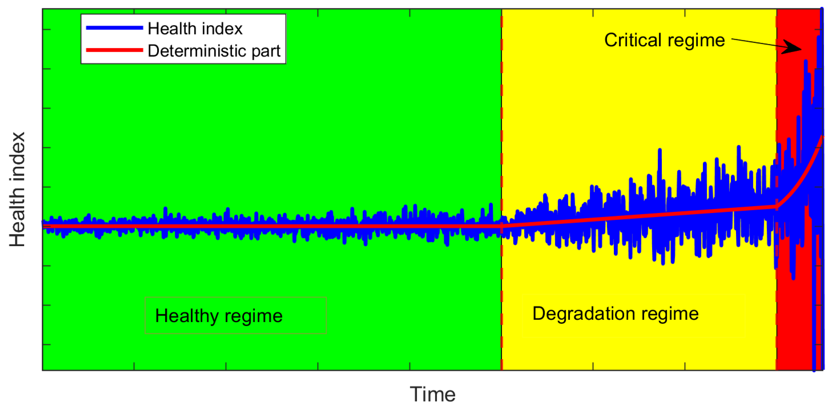
Figure 2.
The flowchart of the proposed methodology (each block of this diagram is described in detail in the following).
Figure 2.
The flowchart of the proposed methodology (each block of this diagram is described in detail in the following).
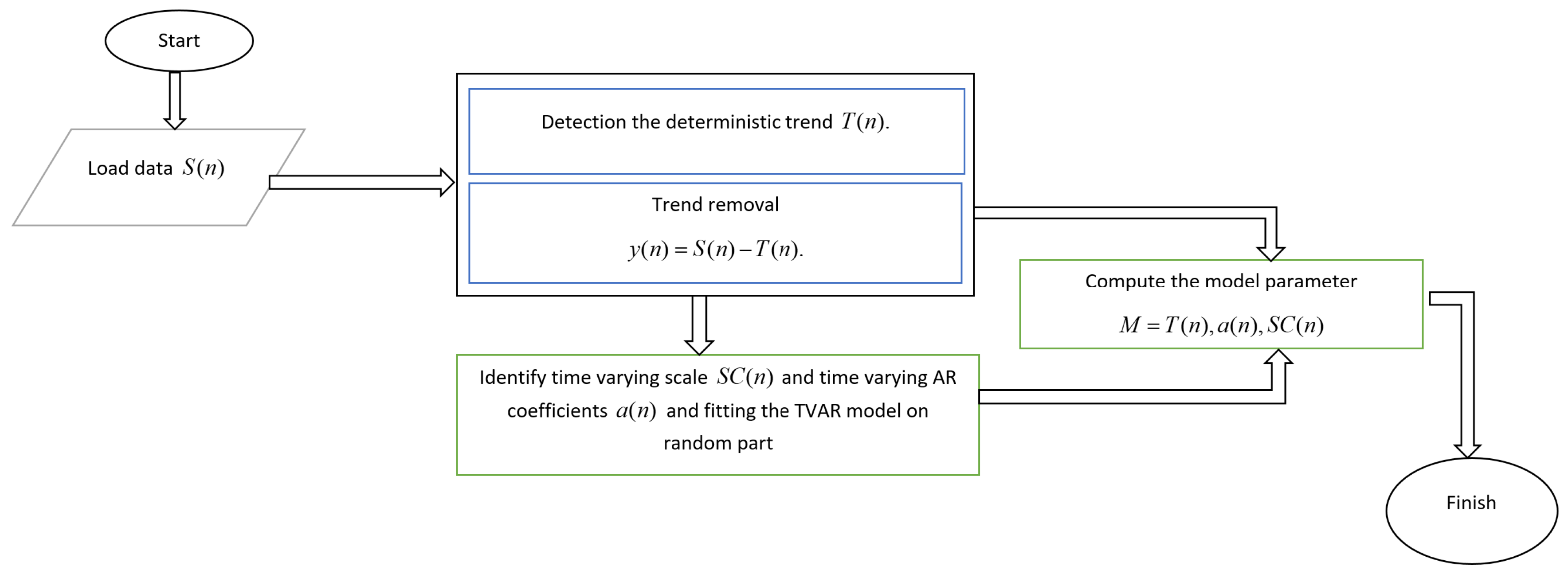
Figure 3.
Generated HI, (a) simulated health index (HI), (b) deterministic component of simulated HI, (c) random component of simulated HI, (d) scale (variance) of simulated HI, (e) AR coefficient of simulated HI.
Figure 3.
Generated HI, (a) simulated health index (HI), (b) deterministic component of simulated HI, (c) random component of simulated HI, (d) scale (variance) of simulated HI, (e) AR coefficient of simulated HI.
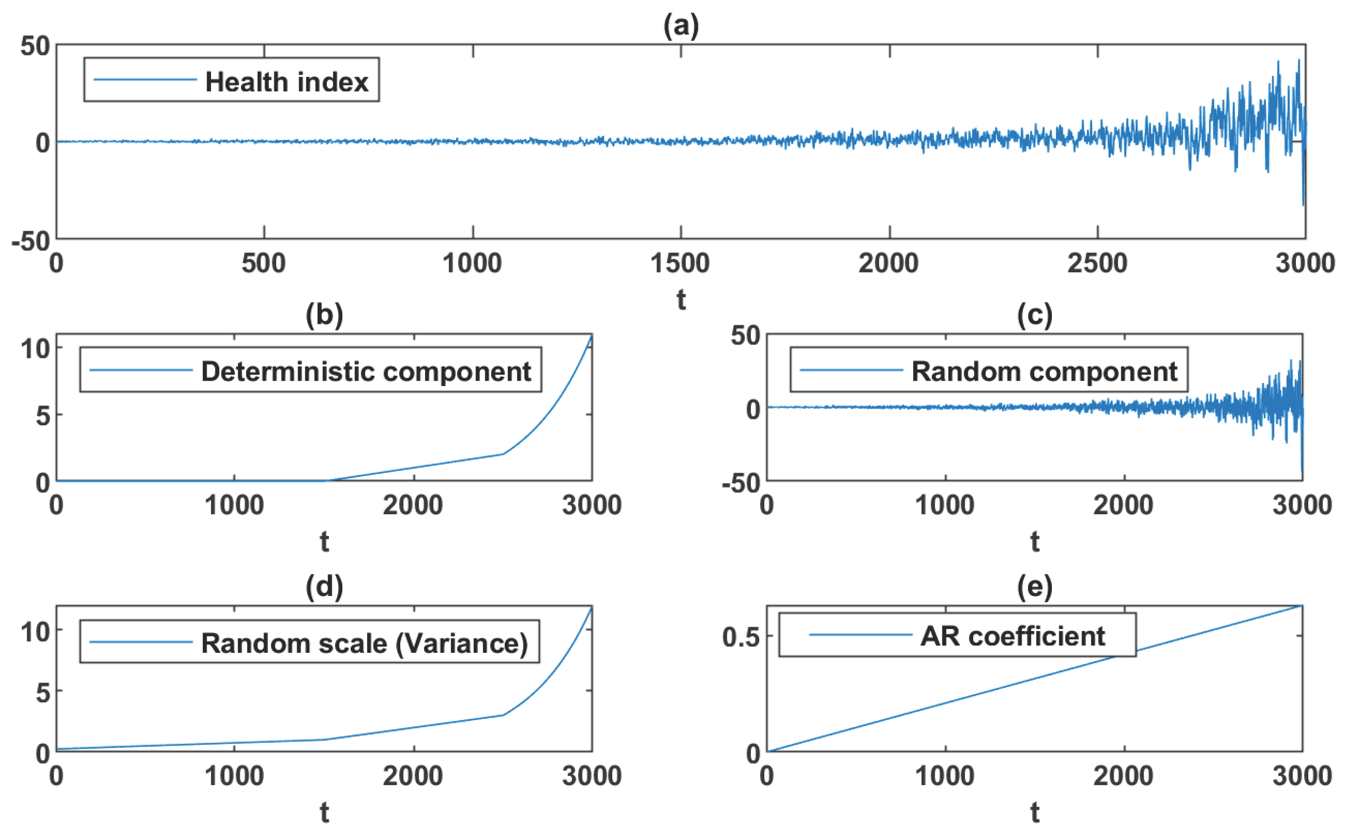
Figure 4.
Results of proposed approaches on simulated Health index (HI), (a) trend (deterministic component) identification, (b) identified random component, (c) identified scale (variance) of random component, (d) identified AR coefficient.
Figure 4.
Results of proposed approaches on simulated Health index (HI), (a) trend (deterministic component) identification, (b) identified random component, (c) identified scale (variance) of random component, (d) identified AR coefficient.
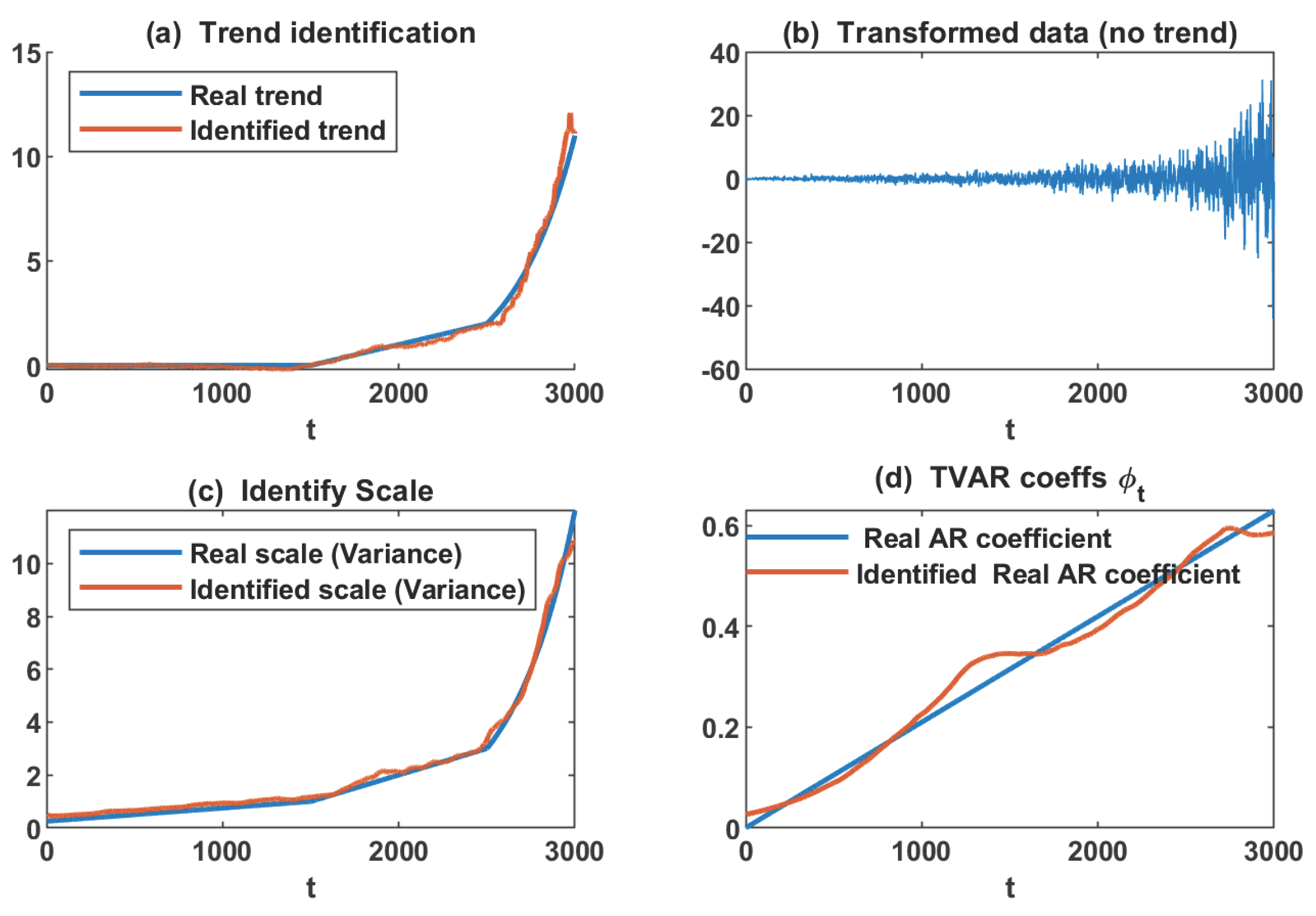
Figure 5.
Results of the proposed procedures on 100 simulated Health index, (trend, variance(scale), AR (1) coefficient). Left column: the proposed method, and the right column: the evaluation of the results by RMSE (trend and variance (scale)) by boxplots.
Figure 5.
Results of the proposed procedures on 100 simulated Health index, (trend, variance(scale), AR (1) coefficient). Left column: the proposed method, and the right column: the evaluation of the results by RMSE (trend and variance (scale)) by boxplots.
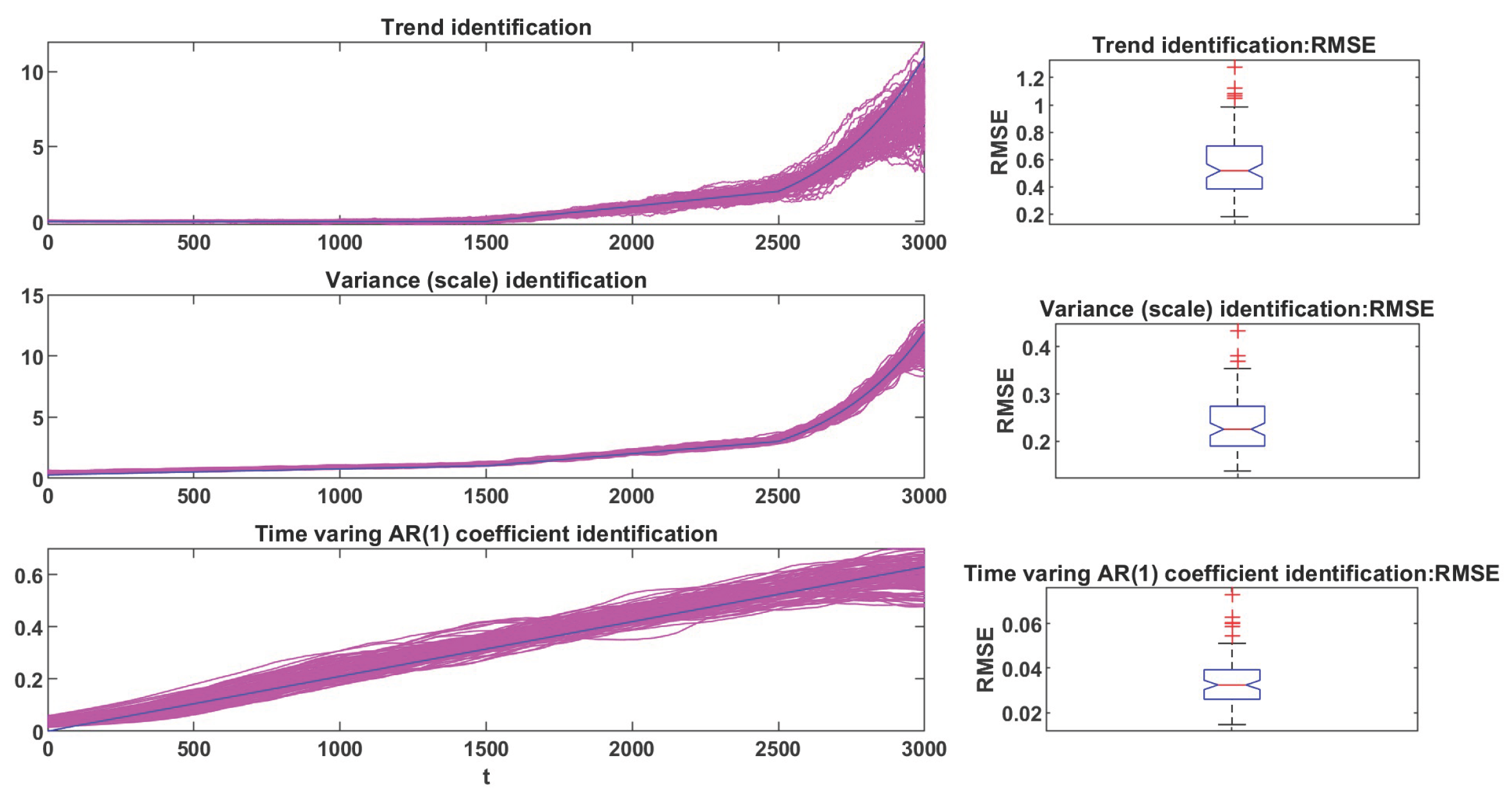
Figure 6.
FEMTO test rigs [37].
Figure 6.
FEMTO test rigs [37].
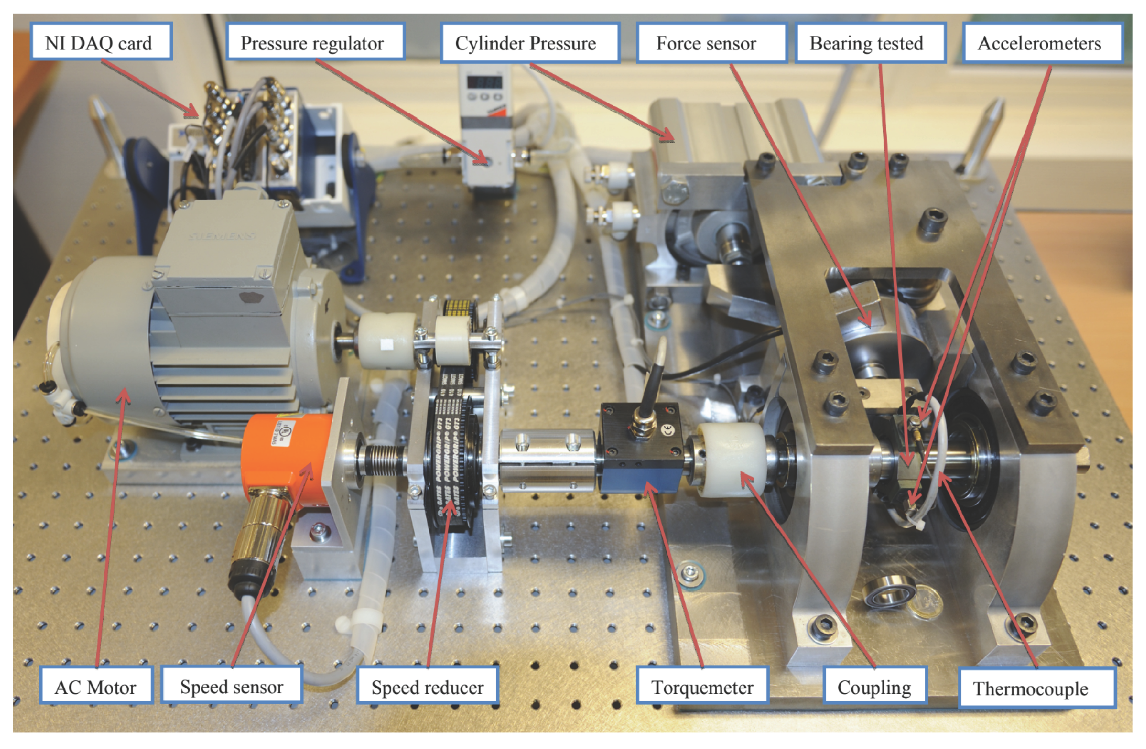
Figure 7.
FEMTO data set, (a) raw bearing run-to-failure vibration signals (b), HI (RMS).
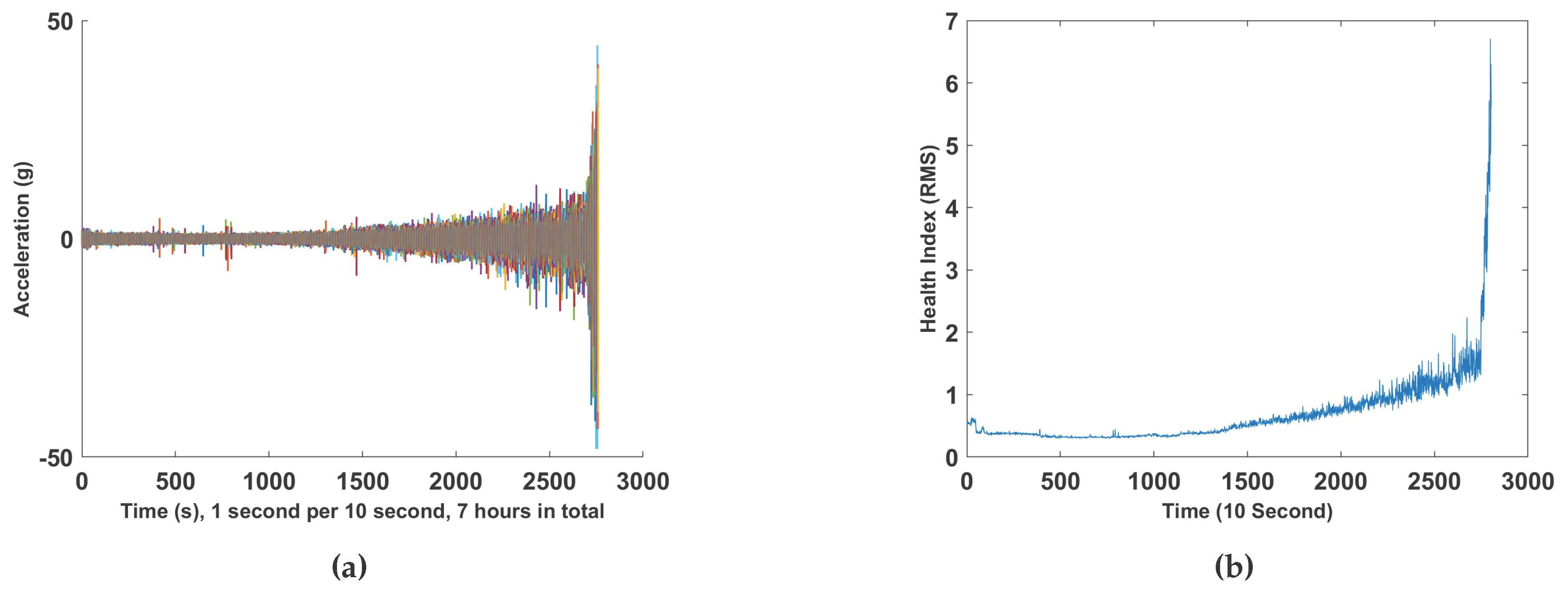
Figure 8.
Wind turbine test rigs [58].
Figure 8.
Wind turbine test rigs [58].
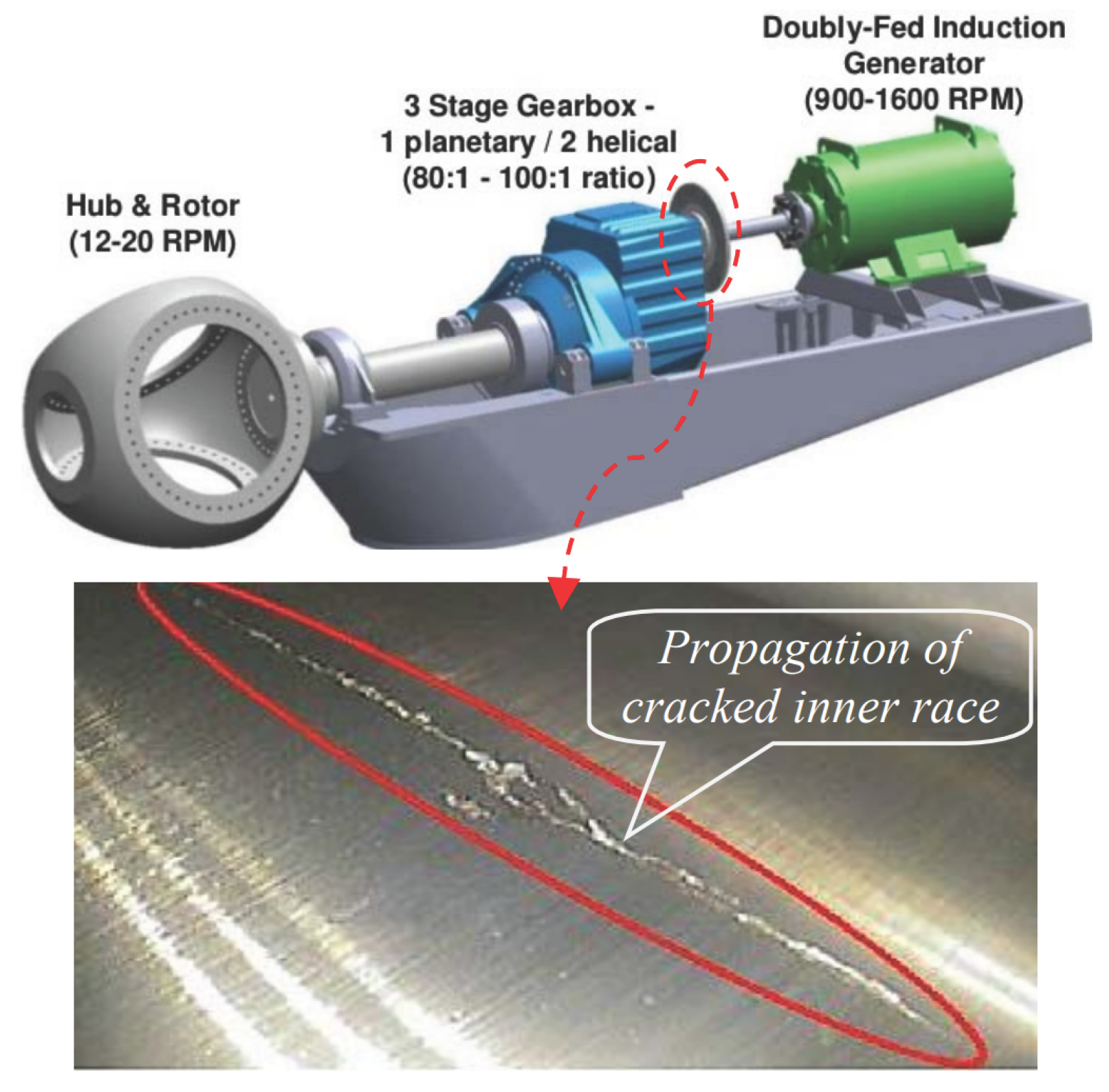
Figure 9.
Wind turbine HI.
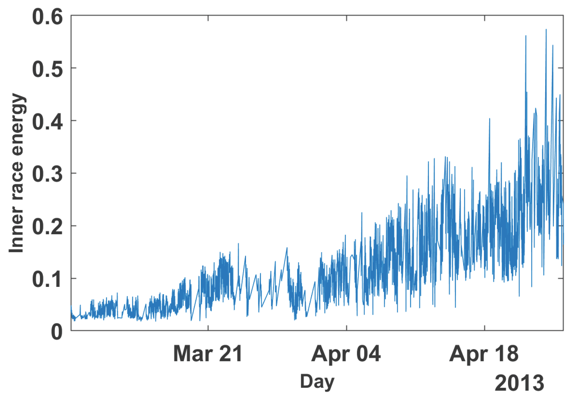
Figure 10.
Results of the applied methodology.
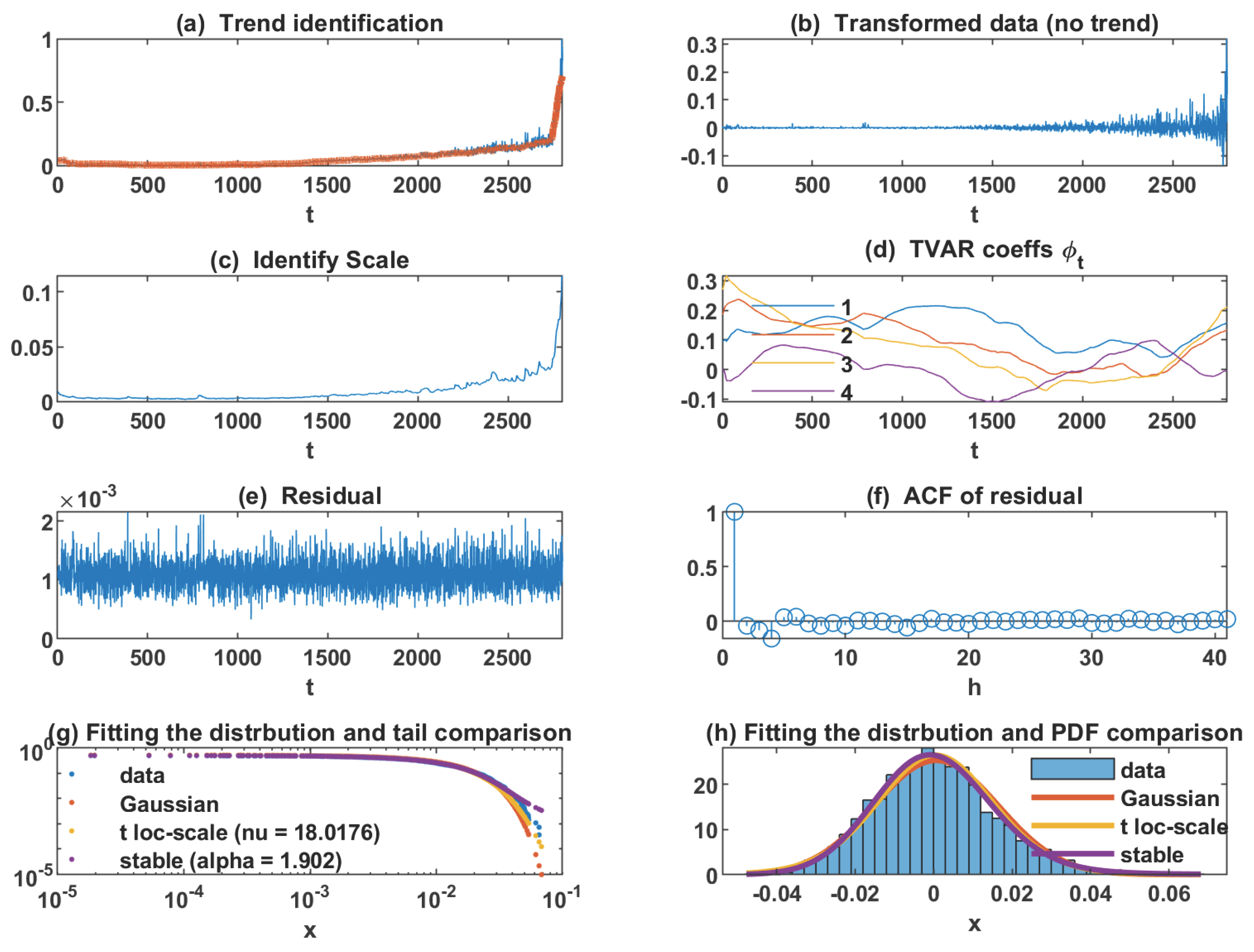
Figure 11.
Constructed quantile lines (blue) on the level of and constructed on the basis of simulated trajectories corresponding to the fitted proposed model.
Figure 11.
Constructed quantile lines (blue) on the level of and constructed on the basis of simulated trajectories corresponding to the fitted proposed model.
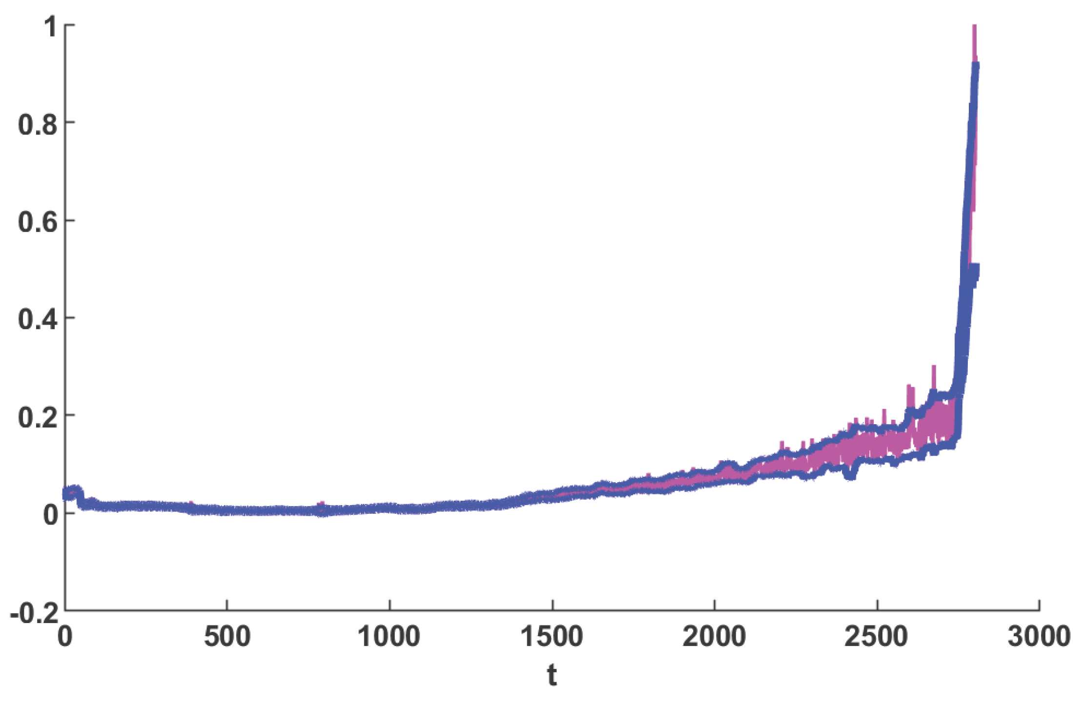
Figure 12.
Results of the applied methodology for wind turbine data set.
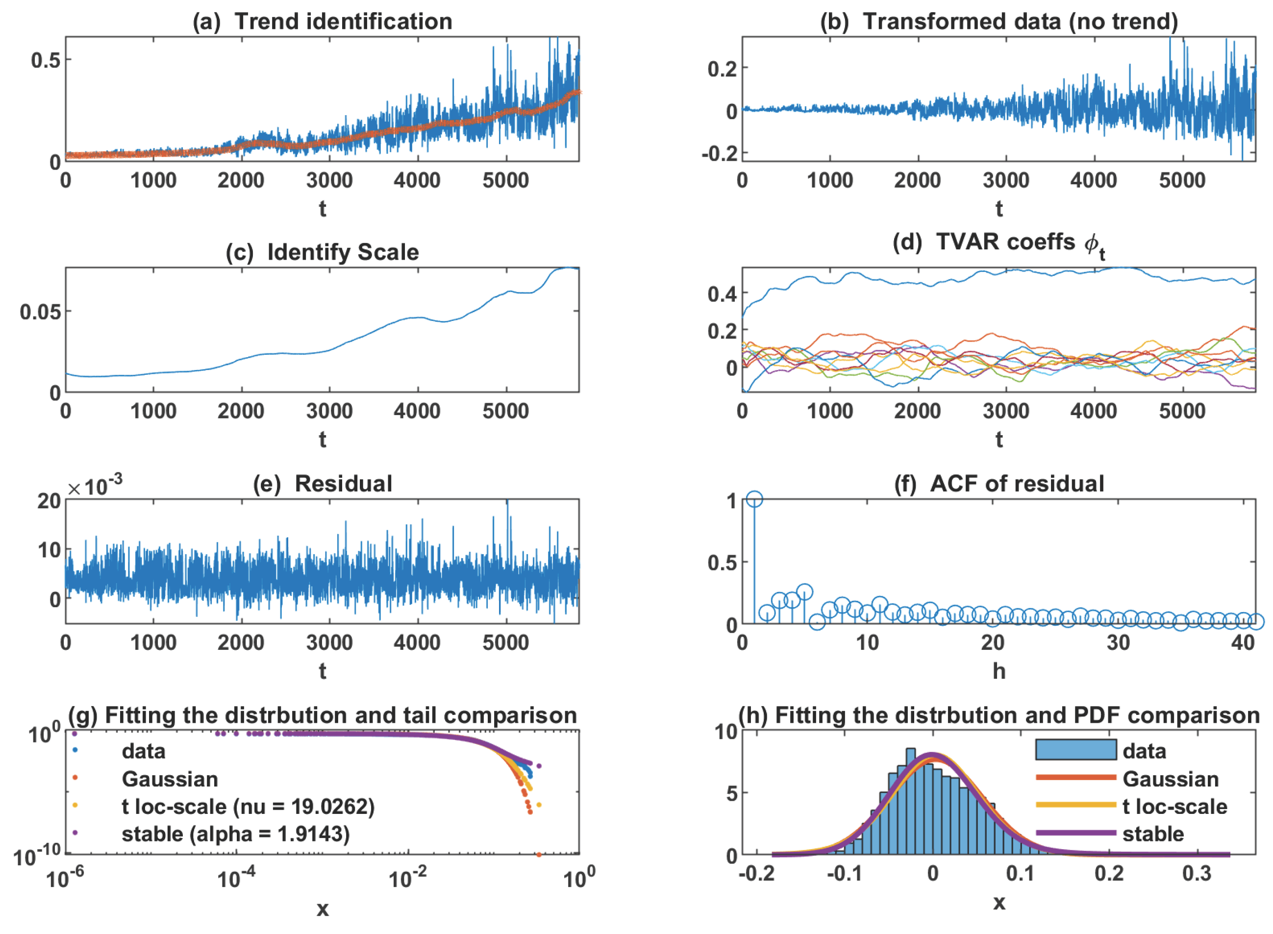
Figure 13.
Constructed quantile lines (blue) on the level of and constructed on the basis of simulated trajectories corresponding to the fitted proposed model.
Figure 13.
Constructed quantile lines (blue) on the level of and constructed on the basis of simulated trajectories corresponding to the fitted proposed model.
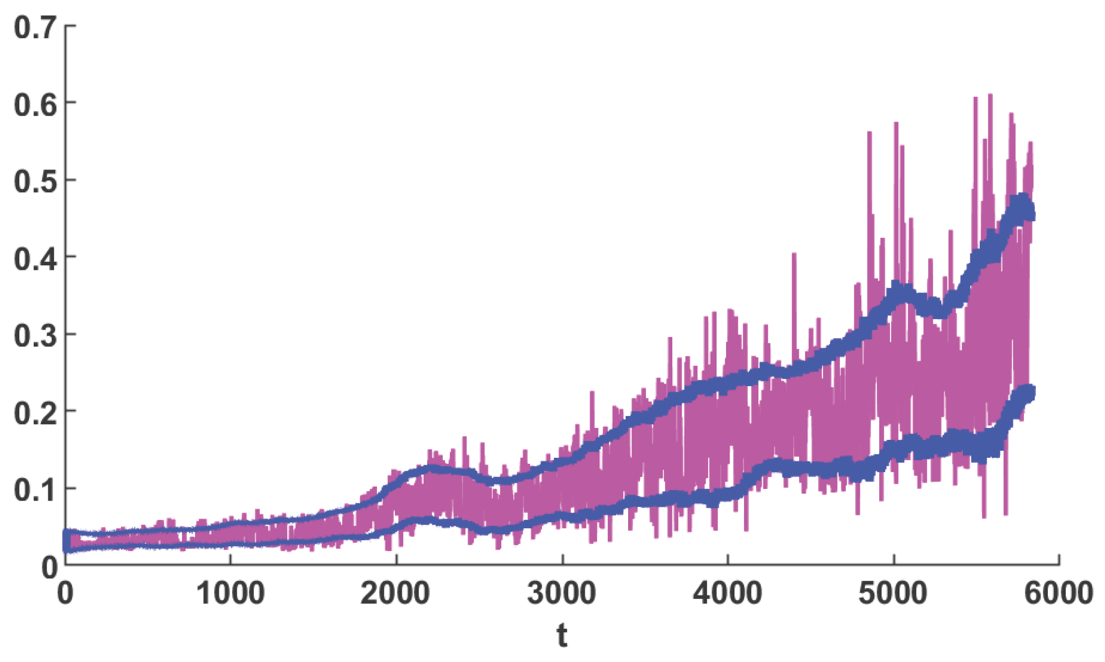
Figure 14.
Comparison between the proposed model and the model of Żuławiński et al. for: (a) 5th and 95th quantiles on the FEMTO dataset, (b) 5th and 95th quantiles on the wind turbine dataset, (c) 95th quantiles on the FEMTO dataset, and (d) 95th quantiles on the wind turbine dataset.
Figure 14.
Comparison between the proposed model and the model of Żuławiński et al. for: (a) 5th and 95th quantiles on the FEMTO dataset, (b) 5th and 95th quantiles on the wind turbine dataset, (c) 95th quantiles on the FEMTO dataset, and (d) 95th quantiles on the wind turbine dataset.
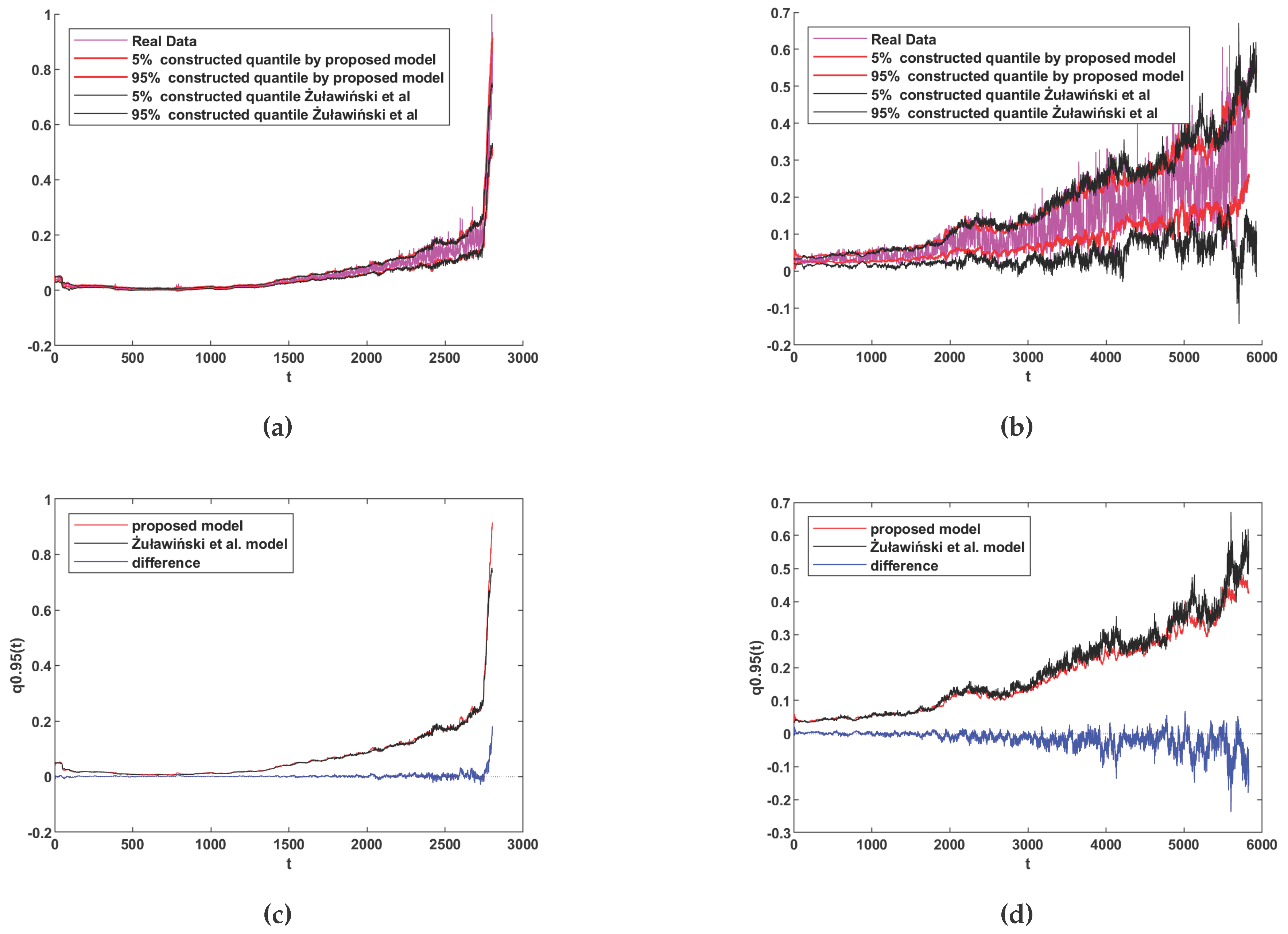

Table 1.
Characteristics of the proposed degradation model.
| Property | Regime 1 | Regime 2 | Regime 3 |
|---|---|---|---|
| Trend | Constant | Linear | Exponential or Polynomial |
| Scale | Nearly constant | Linearly growing | Exponential or polynomial growing |
| Autodependence of noise | White / Colored | White / Colored | White / Colored |
| Noise distribution | Gaussian | Gaussian | Gaussian |
Disclaimer/Publisher’s Note: The statements, opinions and data contained in all publications are solely those of the individual author(s) and contributor(s) and not of MDPI and/or the editor(s). MDPI and/or the editor(s) disclaim responsibility for any injury to people or property resulting from any ideas, methods, instructions or products referred to in the content. |
© 2025 by the authors. Licensee MDPI, Basel, Switzerland. This article is an open access article distributed under the terms and conditions of the Creative Commons Attribution (CC BY) license (http://creativecommons.org/licenses/by/4.0/).
Copyright: This open access article is published under a Creative Commons CC BY 4.0 license, which permit the free download, distribution, and reuse, provided that the author and preprint are cited in any reuse.


