
Submitted:
21 May 2025
Posted:
21 May 2025
You are already at the latest version
Abstract
The non-monotonic behavior of amperometric enzyme-based biosensors under uncompetitive substrate inhibition is investigated computationally using a two-compartment model consisting of an enzyme layer and an outer diffusion layer. The model is based on a system of reaction-diffusion equations that includes a nonlinear term associated with non-Michaelis-Menten kinetics of the enzymatic reaction and accounts for the partitioning between layers. In addition to the known effect of substrate inhibition, where the maximum biosensor current differs from the steady-state output, it has been determined that external diffusion limitations can also cause the appearance of a local minimum in the current. At substrate concentrations greater than both the Michaelis-Menten constant and the inhibition constant, and in the presence of external diffusion limitation, the transient response of the biosensor, after immersion in the substrate solution, may follow a five-phase pattern depending on the model parameter values: it starts from zero, reaches a global or local maximum, decreases to a local minimum, increases again, and finally decreases to a steady intermediate value. The biosensor performance is analyzed numerically using the finite difference method.
Keywords:
amperometric biosensor
; substrate inhibition
; diffusion limitation
; transient response
; mathematical modeling
; computational simulation
1. Introduction
Enzyme-based amperometric biosensors were the first type of biosensors developed and remain the most popular due to their simplicity, ease of production, and low cost [1,2,3]. They measure changes in the output current at the working electrode caused by the direct oxidation or reduction of biochemical reaction products. The amperometric response is typically proportional to the analyte (substrate) concentration in a buffer solution [2,4,5,6]. These devices have found widespread applications in clinical, environmental, industrial, toxin detection and other fields [3,7,8,9,10,11].
Most biosensors operate according to the Michaelis-Menten kinetics scheme,
where E is an enzyme, S is a substrate, is an enzyme-substrate complex, is a reaction product, and , and are the rate constants [2,4,5,7].
Often, the kinetics of the enzyme-based biosensors are much more complicated than in the simplest scheme (1). Different substances may act as inhibitors and cause a reduction in the rate of an enzyme-catalyzed reaction [6,8,12]. The substrate in many enzyme-catalyzed reactions behaves as an inhibitor. In addition to the scheme (1), the interaction of the enzyme-substrate complex (ES) with other substrate molecule (S) following the generation of a non-active inhibitory complex (ESI) may produce one of the simplest non-Michaelis-Menten scheme of the enzyme action,
and are the rate constants [2,3,6,8].
Understanding the kinetic peculiarities of biosensors is crucial in their design and optimization [13,14,15]. Mathematical modeling has proven to be a useful tool to study the effect of enzyme inhibition [10,11,16,17,18,19,20]. Various approaches have been applied for the biosensor modeling [21,22,23,24,25]. Actual biosensors with uncompetitive substrate inhibition have already been modeled at various, often steady-state, conditions [26,27,28,29]. The amperometric biosensors utilizing the enzyme with the substrate inhibition have also been modeled at the external diffusion limitation and the steady-state [10,16] as well as the transition conditions [25,30,31].
In particular, Kulys showed that a multi-steady-state response can be generated at the electrode surface under external diffusion limitations when the substrate concentration is much greater than the Michaelis-Menten constant, assuming an extremely thin enzyme layer [16]. However, to the best of our knowledge, only non-monotonic transient responses featuring a maximum followed by a final steady-state current have been simulated [19,26,30,31,32,33]. In such cases, the response typically follows a three-phase pattern: starting from zero, reaching a maximum, and finally decreasing to a steady value.
When modeling practical biosensors, multi-layer models are usually required to achieve sufficient accuracy of the model [26,34,35]. Nevertheless, even mono-layer models that neglect external mass transport by diffusion have still been used in various applications in recent years due to the model simplicity [18,19,33,36,37,38,39,40]. However, external mass transport by diffusion significantly influences the dynamics of the catalytic processes in enzyme-loaded systems in general and biosensor response and sensitivity in particular [9,41,42,43,44,45]. Fortunately, mass transport through several outer diffusion layers can be rather effectively approximated by a single diffusion layer with effective diffusion coefficients [46,47,48]. As a result, two-compartment models have been widely used in biosensor modeling [10,34,49,50,51,52,53,54].
The aim of this work was to investigate in detail the influence of substrate inhibition, in conjunction with internal and external diffusion limitations, on the transient response of enzyme-based amperometric biosensors. This study focuses on the conditions under which the transient response of the biosensor, after being immersed in a substrate solution, exhibits a complex, multi-phase pattern, characterized by the appearance of a local minimum, a local maximum, or even both.
At transient conditions, a biosensor is mathematically modeled by a two-compartment model comprising a mono-enzyme layer where the enzyme reaction as well as the mass transport by diffusion take place, and a diffusion-limiting region, where only the mass transport by diffusion takes place. The model is based on a system of reaction-diffusion equations that includes a nonlinear term associated with non-Michaelis-Menten kinetics of the enzymatic reaction and involves partitioning between layers. The performance of the treated system is analyzed numerically using the finite difference technique [55,56], and the simulation results are compared with previous studies on biosensors under substrate inhibition [16,19,26,30,31].
2. Mathematical and Computational Modelling
2.1. Biosensor Principal Structure
An amperometric biosensor is considered an electrode and a relatively thin layer of an enzyme (enzyme membrane) applied onto the electrode surface [2,4,6,7,9]. The model involves three regions: the enzyme layer, where the enzymatic reaction as well as the mass transport by diffusion takes place, a diffusion-limiting region where only the mass transport by diffusion takes place, and a convective region where the analyte concentration is maintained constant [30,31]. The schematic view of the modeled biosensor is presented in Figure 1, where and stand for the thicknesses of the enzyme and outer diffusion layers, respectively.
In the enzyme layer, we consider the enzyme-catalyzed reactions (1) and (2). At the electrode surface, the electro-active product is converted into a species having no influence on the biosensor response, and electrons are released,
where n is the number of electrons transferred in the reaction.
Some reactions in the network (1), (2) and (3) are very fast, while others are considerably slower [2,4,6,7,9]. The large difference in timescales in the reaction network creates difficulties in simulating the temporal evolution of the network and for understanding the basic principles of its operation. To sidestep these problems, the quasi-steady-state approximation (QSSA) is often applied [57,58].
Assuming the QSSA, the concentration of the enzyme (E) and intermediate complexes (ES and ESI) do not change with time, and the rate of biochemical reaction is then expressed by the following equation of non-Michaelis-Menten kinetics:
where S is the substrate concentration, is the maximal enzymatic rate, is the total enzyme concentration, is the Michaelis constant, and is the inhibition constant (ESI dissociation constant) [4,31,59].
At so low substrate concentrations as and , the nonlinear reaction rate in (4) reduces to the first-order reaction rate , while at so high concentrations as and , the rate becomes independent of the substrate concentration, i.e., zero-order kinetics. When , the inhibitory term in the denominator of the rate equation becomes significant, and the reaction rate starts to decline, even though substrate concentration is still increasing. The influence of inhibition on the overall biochemical process decreases with an increasing inhibition constant , and the non-Michaelis-Menten kinetics approaches the Michaelis-Menten kinetics as . Focusing on the influence of substrate inhibition, the analysis is limited to substrate concentrations greater than the inhibition constant .
In the two-compartment (two-layer) model, the diffusion layer is often treated as the Nernst diffusion layer [9,55,60]. But it can also be treated as a semi-permeable (diffusion-limiting) membrane if the outer Nernst diffusion is neglected [25,34,43,55,61], although the Nernst layer’s zero thickness cannot be achieved in practice [62].
Sometimes, mathematical models of biosensors involve both the outer membrane and the Nernst diffusion layer [26,47,48,63]. However, the mass transport through several diffusion layers can be rather efficiently approximated by a single diffusion layer with effective diffusion coefficients, and a multi-compartment model can be reduced to a two-compartment model [46,47,48]. Therefore, the effects investigated here can also be applied to amperometric biosensors modeled by several diffusion layers including outer membranes and the Nernst diffusion layer.
2.2. Mathematical Model
Assuming symmetrical geometry of the electrode, enzymatic, and diffusion layers, along with a homogeneous distribution of the immobilized enzyme within the enzyme membrane, results in a two-compartment mathematical model defined in a one-dimensional spatial domain. This model is formulated as an initial boundary value problem that describes the dynamics of substrate and product concentrations [8,25,34,64,25].
2.2.1. Governing Equations
The dynamics of the concentrations of the substrate S and product P in the enzyme layer is described by a system of reaction-diffusion equations (),
where and are the concentrations of the substrate and the product in the enzyme layer, and are the diffusion coefficients, is the thickness of the enzyme layer, and is the reaction rate as defined in (4) [8,34,59].
2.2.2. Boundary Conditions
In the bulk, the concentrations of the substrate and the product remain constant during the biosensor operation (),
where is the concentration of the substrate in the bulk.
At the interface between adjacent layers, the exiting and entering fluxes of the substrate and product are assumed to be equal, while the concentrations on either side of the interface are related through formal partition coefficients and ( [63,64,65,66,67],
2.2.3. Initial Conditions
Two different initial conditions corresponding to two modes of biosensor operation are considered.
In the first mode, the biosensor is assumed to be permanently immersed in a buffer solution, and its operation begins when the analyte (substrate) is introduced at into the buffer solution,
This setup simulates injection analysis (IA) or real-time monitoring, where the analyte arrival initiates the biosensor transient response [8,9,10,18,26,51,70].
The second type of operation is common in batch analysis (BA) when the biosensor is directly immersed in a buffer solution containing the analyte [8,9,20,53,71]. The biosensor operation starts responding to the analyte from the moment of immersion. In this case, initial conditions (10) have to be replaced with
2.3. Biosensor Response
The amperometric electrode measures the faradaic anodic or cathodic current [2,8,59]. The density of the output current at time t can be obtained explicitly from Faraday’s and Fick’s laws,
where n is the number of electrons involved in a charge transfer at the electrode surface, and F is the Faraday constant [8,34,69].
The system (5)-(9) approaches a steady-state as [8,34,59],
where is the density of the steady-state output current.
Since the transient current in the case of the enzyme inhibition can be a non-monotonic function of time, the maximal current has also been used as a characteristic for this kind of biosensor [19,26,30,31,32,33]. Aiming to determine conditions under which biosensor response follows a multi-phase pattern, the number of extrema in transient output current was studied. A local or global maximum of otput current occurs at time if for all t near , while a local minimum occurs at that time if for all t near . is considered as the total count of maxima and minima that the function has at ,
where denotes the set cardinality and the condition for defining the set.
In the specific case of a monotonic output current , = 0. In the case of a three-phase pattern, when the output current starts from zero, reaches a maximum, and then decreases to a steady value, = 1. = 2 when the biosensor response approaches a four-phase pattern, exhibiting a local minimum in addition to the maximum.
2.4. Dimensionless Model Parameters
In order to obtain the main governing parameters of the mathematical model, a dimensionless model is typically derived [60,63]. The two-compartment model mathematical model (5)-(9) was expressed in the dimensionless form by rescaling time, space [25,31,43]. The following governing dimensionless parameters were obtained:
where is the dimensionless Damköhler number (the Thiele modulus squared) or the diffusion module, and are the Biot numbers for the substrate and product, respectively [34,69,72,73]. The model equations (5)-(9) in dimensionless form are presented in the Appendix. All the dimensional and dimensionless model parameters are listed in Table A1.
The dimensionless factor essentially compares the rate of intrinsic enzyme reaction () with the rate of diffusion through the enzyme layer (). The enzyme kinetics controls the biosensor response when , while the response is under internal diffusion control or limitation when [2,8,34,42,73]. Rearranging the expression of gives the timescales of the enzymatic reaction and internal diffusion.
The Biot number is a dimensionless parameter widely used to compare the relative transport resistances of external and internal diffusion [9,41,42,44,45,72]. Since the mass transport properties of the substrate and product are generally different, separate Biot numbers have been introduced, although they are often assumed to be identical [41,43,44,45,48,74]. The mass transport by diffusion in the enzyme layer is slower than in the diffusion layer at large Biot number values, while low values indicate slower diffusion in the diffusion layer than in the enzyme layer [9,42,72].
2.5. Numerical Simulation
Due to the nonlinearity of the governing equations (5) the initial boundary value problem (5)–(11) can be analytically solved only for specific values of the model parameters [10,34,55]. Hence, the problem was solved numerically.
To find a numerical solution to the problem (5)–(11), a non-uniform discrete grid was introduced in space and time. A semi-implicit linear finite difference scheme has been built as a result of the difference approximation of the model equations [25,31,75]. The resulting system of linear algebraic equations was solved efficiently by the Thomas (the tridiagonal matrix) algorithm [55]. To have an accurate and stable result, it was required to use a small step size in x direction at the boundaries , and , where the concentration gradients are larger than the gradients away from those boundaries. Further from these boundaries, an exponentially increasing step size was used [25,48,74].
Although the time step is restricted by the partition conditions (8) [76,77,78], it was reasonable to apply an increasing step size in the time direction [79], as the biosensor action follows the steady-state assumption as . The final step size in time was in a few orders of magnitude higher than the first one [43]. The density of the steady-state output current was approximated by the output current calculated at the moment, when the normalized absolute current slope value fell below a given small value [25,34].
The numerical simulator has been programmed in Java language [80]. The numerical solution was validated using exact analytical solutions known for specific cases of the first and zero-order reaction rates at the steady-state conditions [34,43] and numerical solutions derived for a two-compartment model of amperometric biosensors at transient conditions [10,31,34]. Approximate analytical solutions, obtained for the corresponding one-compartment model of biosensors with substrate inhibition at steady-state [28,36,37] and transient conditions [33], were also used for validation of the numerical solution.
The simulation results have been visualized using Origin [81].
3. Results and Discusion
To investigate the non-monotonic behavior of amperometric enzyme-based biosensors under uncompetitive substrate inhibition, in conjunction with internal and external diffusion limitations, the biosensor action was simulated across a wide range of key dimensionless model parameter values, using the following typical assumptions for the parameter values: [1,30,31,43,48]:
3.1. Temporal Dynamics of Biosensor Response
Figure 2 shows typical temporal dynamics of the biosensor current I simulated at the following ten values of the substrate concentration : 0.1, 0.2, 0.3, 0.4, 0.5, 0.6, 0.7, 1, 2 and 3 , with fixed parameters = , = , and , in both types of analysis, injection (IA) and batch (BA). The corresponding normalized values of the substrate concentration are indicated on the curves in Figure 2. All the other model parameters were defined in (16). These simulations were performed under mixed control, involving both enzyme kinetics and internal diffusion (). On the other hand, mass transport in the outer diffusion layer was slower than in the enzyme layer, as indicated by .
One can see in Figure 2 a noticeable difference in the dynamics of the biosensor response when changing the substrate concentration . The shape of the curves also depends significantly on the mode of analysis, i.e., on the initial conditions (10) or (11). However, the steady-state response is independent of the analysis mode, as the steady-state solution of the initial boundary value problem (5)–(8) is unaffected by those initial conditions [8,25,34,55].
At the beginning of biosensor operation, the output current becomes noticeably slower in IA mode than in BA mode. The delay consists of about 6 - 10 s. This delay in the transient response can be attributed to the diffusion time required for the substrate to pass through the outer diffusion layer and reach the enzyme layer in IA mode [4,29,59]. In contrast, in BA, the substrate contacts the enzyme layer immediately at . The corresponding steady-state times are approximately the same, though they noticeably depend on the substrate concentration.
In IA (Figure 2(a)), at relatively high substrate concentrations (), the response follows a three-phase pattern: starting from zero, reaching a maximum, and finally decreasing to a steady value. The output current, after reaching its maximum, enters the descending limb of the bell-shaped curve characteristic of substrate inhibition. In the case of low and moderate substrate concentrations ( in Figure 2(a)), the biosensor current monotonically approaches steady-state. On the other hand, Figure 2(a) shows nonmonotonic behavior of the steady-state current. At substrate concentrations corresponding to the three-phase pattern (), the steady-state current decreases with increasing , whereas at lower concentrations (), it increases with increasing . These aspects of the biosensor with uncompetitive substrate inhibition are well known [19,26,30,31,32,33].
Figure 2(b) shows noticeably more complex dynamics of the biosensor current in BA mode than in IA. Even at relatively low substrate concentrations (), the output current is nonmonotonic. At slightly greater concentration , the output current becomes a monotonously increasing function of time t, but has an extra inflection point ( s) where the curve changes from concave down to concave up.
In the case of relatively high substrate concentrations (), the biosensor response exhibits a local minimum and follows a four-phase pattern. At higher concentrations , the response approaches even a five-phase pattern, although the oscillations at are only slight. Specifically, at the transient current starts from zero, reaches a global maximum of at s, decreases to a local minimum of at s, increases to a local maximum of at s, and finally decreases to a steady value of . Thus, the variation between the local extrema and the steady value is only . At a higher concentration of , this variation is even smaller.
3.2. Effect of Internal Diffusion Limitation
Figure 2 shows the influence of substrate concentration on the dynamics of output current at a fixed maximal enzymatic rate of = , which corresponds to a diffusion module equal to unity (). To investigate the effect of the diffusion module on the transient response of the amperometric biosensors, the response was simulated at very different values of . This allowed the transition from enzyme kinetics control () to internal diffusion control () to be observed, while keeping all other parameters the same as those used in the simulations depicted in Figure 2. Figure 3 shows the number of extrema calculated from the simulated responses in both modes of analysis, IA and BA.
As one can see in Figure 3(a), the transient output current exhibits one or even no local extremum in IA, when the diffusion module changes in four orders of magnitude, from to 100, and the dimensionless substrate concentration changes from 1 to 30. When the biosensor acts under the internal diffusion limitation (), the response follows a two-phase pattern (): starting from zero increases to a steady value. A three-phase pattern () is observed when the biosensor response is governed by enzyme kinetics or mixed control (), although it also depends on the substrate concentration. The yellow line in Figure 3 represents an approximate boundary between the two values of , 0 and 1, i.e., between model parameter values that result in either two-phase or three-phase patterns. This yellow line is a linear approximation of the boundary,
The relationship (17) between the substrate concentration and the diffusion module , resulting in changes in the number of response phases, is approximately linear when the biosensor operates in IA mode, as defined by (17) (Figure 3(a)). Similar dependences of the substrate concentration on the diffusion module have already been observed [26,31,33,39,40]. In particular, it was found that the minimum dimensionless substrate concentration at which the response reaches its maximum is a monotonically increasing function of [31]. In the case of BA (Figure 3(b)), that relation is noticeably more complicated as the number of extrema varies between zero and three, indicating that the number of phases in the response pattern ranges between two and five. In particular, at , increasing the normalized substrate concentration from 1 to 30 results in the number of extrema changing in the following sequence: 1, 0, 1, 2, 3. This can also be noticed in Figure 2(b).
Although the variation in the number of extrema differs noticeably among the analysis modes, at relatively low substrate concentrations () and very low values of the diffusion module (), the number is practically invariant across analysis mode, as observed in the lower left corners of Figure 3(a) and Figure 3(b).
To observe the effect of the diffusion module on the shape of the transient response, the biosensor action was simulated at different values of , while keeping the substrate concentration fixed at a relatively high level ( = = 10, ), where the inhibition plays a significant role in the biosensor response. The simulation results are shown in Figure 4.
One can see in Figure 4(a), in IA, the transient output current exhibits a global maximum for , whereas it is a monotonously increasing function of time t for greater values of the diffusion module , as it was predicted in Figure 3(a). In BA (Figure 4(b)), for , the shape of is similar to that observed in IA mode (Figure 4(a)), although the function in BA has additional local extremums, which are close to steady values. However, at slightly greater values of (), the transient current ehibits a noticeable peak in BA. At high values of the diffusion module (), when the response is govern by internal diffusion control, the output current exhibits only a global maximum, following a two-phase pattern.
On the other hand, at high values of the diffusion module (), the transient response in IA becomes practically invariant to , whereas in BA, the response dynamics still noticeably depend on . Maintaining the analytical capability of biosensors for as long as possible is very important [2,4,7]. Typically, the maximal enzymatic rate decreases over time due to enzyme inactivation [70,82]. Therefore, ensuring the stability of the biosensor response (the biosensor resistance) across a range of values is crucial [25,33,37,39,40,82]. Since directly influences , it is essential to maintain a stable response even when undergoes slight variations.
In particular, at two significantly different values of , namely and 5, the response of a biosensor operating under BA conditions follows a five-phase pattern ( = 3). However, in the case of (and for as well), the local minimum is barely noticeable, whereas for , all extrema and all five phases are clearly observable. This is particularly important in practical applications of amperometric biosensors, as oscillations in the biosensor response may complicate the use of the calibration curve [15,16]. On the other hand, analyzing both the steady-state and the maximal biosensor currents can significantly extend the calibration curve when using intelligent biosensors [15,30,31,83].
3.3. Effect of External Diffusion Limitation
To investigate the influence of external diffusion limitations on the behavior of amperometric enzyme-based biosensors, the biosensor response was simulated by varying the partition coefficient over two orders of magnitude, from to . This variation caused the governing dimensionless Biot number to change from to 10, representing a shift from external to internal mass transfer dominance [9,72]. The substrate concentration was also independently varied from 0.025 to 3 mM. Simulations were conducted for both types of analysis, injection (IA) and batch (BA), using fixed parameters of = and . Figure 5 shows the number of extrema calculated from the simulated responses.
As one can see in Figure 5(a), in IA, the dependence of the number of extrema of the transient current on the Biot number is rather similar in shape to that on the diffusion module . In IA, when the mass transport by diffusion in the diffusion layer is notably faster than in the enzyme layer (), the response follows a two-phase pattern (). At smaller values of , when the diffusion in the outer diffusion layer is comparable with or slower than that in the enzyme layer (), the response follows a three-phase pattern (), although it also depends on the substrate concentration. The yellow line in Figure 5(a) represents an approximate boundary between the two values of , 0 and 1,
In the case of BA (Figure 5(b)), the relationship between the number of extrema, the Biot number , and the substrate concentration is noticeably more complex. The number varies between zero and three, and the boundary between the regions where and is clearly nonlinear. Nevertheless, the boundary (yellow line) between areas indicated as and is similar to that observed in IA (Figure 5(a)) between and . At relatively high substrate concentrations (), the number of response phases is the same in both modes of analysis, IA and BA, except when , where the number of phases in BA is greater than in IA.
To observe the effect of the Biot number on the shape of the transient response, the biosensor performance was simulated at nine values of , while keeping the substrate concentration fixed at a relatively high level ( = = 10). The simulation results are shown in Figure 6.
Figure 6(a) shows, that in IA at , the transient biosensor current exhibits a global maximum for , whereas it is a monotonously increasing function of time t for greater values of the Biot number , as it was also shown in Figure 5(a).
In BA (Figure 6(b)), three extrema can be observed only for the smallest value of the Biot number of . However, a local minimum and local maximum differ by less than 1 percent. At no local extrema are observed but an extra inflection point ( s) is observed where the curve changes from concave down to concave up. When , the transient output current has only one global maximum (), which occurs noticeably later (at s) than global maximum observed for small values of (at s), and is close to steady-state value. For larger values of (), the global maximum decreasingly approaches the steady-state value.
In addition to the Biot number , the external Thiele modulus (also known as the external Damköhler number and the external diffusion module) is used to compare external and internal mass transport resistances. It relates the characteristic timescale of enzymatic reaction within the enzyme layer to that of external mass transfer, i.e., it represents the ratio between the first-order surface reaction rate () and the rate of the mass transfer through the external diffusion layer () [16,30,44,45]. If , then the external mass transfer is fast, and the system acts in a reaction-limited regime. The enzymatic reaction is fast, and the external diffusion is limiting when . The internal and external Thiele moduli are related through the Biot number for the mass transfer,
The effect of the external Thiele modulus on the behavior of amperometric enzyme-based biosensors was not investigated separately, as it is represented through two other dimensionless parameters: the diffusion module , and the Biot number = .
3.4. Effect of Inhibition
To investigate the effect of inhibition on the behavior of the biosensor transient current, the biosensor response was simulated by varying the inhibition constant over four orders of magnitude, from to , thereby changing the normalized inhibition constant from to 100. The substrate concentration was independently varied from 0.025 to 3 mM, as in numerical experiments discussed above. Simulations were conducted for both types of analysis, injection (IA) and batch (BA), using fixed parameters of = and . At these parameter values, the diffusion module , and the Biot number . Figure 7 shows the calculated number of extrema.
As one can see in Figure 7, the dependence of the number of extrema of the transient current on the inhibition constant differs noticeably from those on the diffusion module (Figure 3) and the Biot number (Figure 5).
In IA (Figure 7(a)), the response follows a three-phase pattern () in most of the entire region of parameter values, . Only at relatively low substrate concentrations and large values of the inhibition constant, the response follows a two-phase pattern (), as in the Michaelis-Menten kinetics. This behavior is reasonable because the influence of inhibition decreases with an increasing inhibition constant. Nevertheless, an increase in the inhibition constant can be compensated for by an increase in the substrate concentration. In a particular case of , the inhibitory term in the reaction rate equation (4) becomes significant when . The relationship between and is nonlinear. The yellow line in Figure 7(a) represents an approximate boundary between the two values of , 0 and 1. This line is a power-law (allometric) approximation of the boundary,
As shown in Figure 7, in the region parameter values and where in IA (i.e., below the yellow line), in BA.
Figure 7(a) shows that, in the particular case of , the transient output current in IA is a monotonically increasing function of time for concentrations , and become a non-monotonic function (with ) at higher concentrations. In the corresponding BA (Figure 7(b)), the number changes with increasing substrate concentration in the following sequence: 1, 0, 2, 3. Notably, occurs in the specific case of . The current dynamics in these cases are also illustrated in Figure 2.
To observe the effect of the inhibition constant on the dynamics of the transient current, the biosensor action was simulated at eleven different values, with the constant substrate concentration held at = 10. The simulation results are depicted in Figure 8.
As seen in Figure 8(a) and Figure 7(a), in IA at , the transient current exhibits a global maximum for all values of the inhibition constant less than 8. Only when becomes comparable to or greater than the concentration () does the output current become a monotonically increasing function of time t.
In BA (Figure 6(b) and Figure 7(b)), the transient current at is monotonic only within a relatively narrow range of the inhibition constant , approximately between 3 and 8. The number of extrema is observed when varies approximately between 0.1 and 0.9. However, the local minimum and maximum differ from the steady-state by only 1 - 2%, although the global maximum is noticeably more pronounced. Such small deviations in local extrema from the steady value can be considered perturbations of the response, influencing the response analysis procedure [15,30,31,83].
4. Conclusions
The two-compartment mathematical model (5)–(11) of amperometric enzyme-based biosensors is useful for investigating the influence of uncompetitive substrate inhibition, in conjunction with internal and external diffusion limitations, on the biosensor response. Deriving the corresponding dimensionless form of the model (A1)–(A7) reveals the main governing dimensionless parameters (15).
The dynamics of the enzymatic system shown in Figure 1 are highly sensitive to internal and external diffusion limitations, enzyme inhibition, and, most notably, the mode of analysis. In injection analysis (IA, real-time monitoring), where the arrival of the analyte initiates the biosensor transient response, the response follows a two- or three-phase pattern. In batch analysis (BA), where the biosensor is directly immersed in a buffer solution containing the analyte, the response may exhibit up to five phases. The number of extrema in the transient output current, as defined by equation (14), is useful for determining the conditions under which the biosensor response follows a multi-phase pattern. The steady-state biosensor current is invariant with respect to the analysis mode (Figure 2).
The non-monotonic (three-phase, ) transient output current of biosensors operating in IA is observed only when the enzyme kinetics predominate in the biosensor response, compared to the internal diffusion, or when the operation is under mixed control (diffusion module ) (Figure 3(a)), the diffusion in the outer diffusion layer is comparable to or slower than that in the enzyme layer (the Biot number ) (Figure 5(a)), and the substrate concentration is comparable to or greater than the inhibition constant (Figure 7(a)), where the current shows a global maximum greater than a steady value (Figure 4(a), Figure 6(a) and Figure 8(a)).
In BA, the monotonic (two-phase, ) transient current is observed only when the biosensor response is notably governed by enzyme kinetics (), mass transport by diffusion in the diffusion layer is faster than in the enzyme layer (), and under specific values of other parameters. Under conditions where biosensors operating in IA follow a three-phase pattern, the transient current in BA can exhibit a maximum five-phase pattern () (Figure 3(b), Figure 5(b) and Figure 7(b)), where the current shows a global maximum, a local minimum, and a local maximum. The global maximum may occur either before or after a local minimum (Figure 4(b), Figure 6(b) and Figure 8(b)).
Oscillations in the transient biosensor response, caused by substrate inhibition and both internal and external diffusion limitations, should be taken into consideration when using the biosensor calibration curve.
Funding
This research received no external funding.
Institutional Review Board Statement
Not applicable.
Informed Consent Statement
Not applicable.
Data Availability Statement
The study did not report any data.
Acknowledgments
The author sincerely thanks Professors Emeritus Juozas Kulys and Feliksas Ivanauskas for their valuable discussions and contributions to the modeling of biosensors.
Conflicts of Interest
The author declares no conflicts of interest.
Abbreviations
The following abbreviations are used in this manuscript:
| E | Enzyme |
| S | Substrate |
| P | Reaction product |
| ES | Enzyme-substrate complex |
| ESI | Inhibitory complex |
| IA | Injection analysis |
| BA | Batch analysis |
| QSSA | Quasi-steady-state approximation |
Appendix A. Dimensionless Mathematical Model
The two-compartment model (5)-(11) was expressed in the dimensionless form by rescaling the time, space, concentrations, and diffusion coefficients as defined in Table A1.
The governing equations (5) in the dimensionless form were then expressed as follows ():
where = .
The diffusion equations (6) take the following form ():
where = , = , = .
The initial conditions specific to IA, as given in (10), take the following form:
The initial conditions (11), which are specific to BA, are transformed to the following conditions:

Table A1.
Dimensional and dimensionless parameters.
| Parameter | Dimensional | Dimensionless |
|---|---|---|
| Time | t, s | |
| Distance from electrode | ||
| Enzyme layer thickness | ||
| Diffusion layer thickness | ||
| Substrate concentration in enzyme layer | ||
| Product concentration in enzyme layer | ||
| Substrate concentration in diffusion layer | ||
| Product concentration in diffusion layer | ||
| Substrate concentration in bulk | ||
| Michaelis-Menten constant | ||
| Substrate inhibition constant | ||
| Maximal enzymatic rate | ||
| Current density | ||
| Steady-state current density | ||
| Diffusion coefficient of substrate in enzyme layer | ||
| Diffusion coefficient of product in enzyme layer | ||
| Diffusion coefficient of substrate in diffusion layer | ||
| Diffusion coefficient of product in diffusion layer | ||
| Partition coefficient for substrate | ||
| Partition coefficient for product | ||
| Biot number for substrate | ||
| Biot number for product | ||
| Diffusion module | ||
| External diffusion module |
References
- Bisswanger, H. Enzyme Kinetics: Principles and Methods, 2 ed.; Wiley-Blackwell: Weinheim, Germany, 2008. [Google Scholar]
- Malhotra, B.D.; Pandey, C.M. Biosensors: Fundamentals and Applications; Smithers Rapra: Shawbury, 2017. [Google Scholar]
- Patra, S.; Kundu, D.; Gogoi, M. (Eds.) Enzyme-based Biosensors: Recent Advances and Applications in Healthcare; Springer Verlag: Singapore, 2023. [Google Scholar]
- Scheller, F.W.; Schubert, F. Biosensors; Elsevier Science: Amsterdam, 1992. [Google Scholar]
- Sadana, A.; Sadana, N. Handbook of Biosensors and Biosensor Kinetics; Elsevier: Amsterdam, The Netherlands, 2011. [Google Scholar]
- Cornish-Bowden, A. Fundamentals of Enzyme Kinetics, 3 ed.; Portland Press: London, 2004. [Google Scholar]
- Turner, A.P.F.; Karube, I.; Wilson, G.S. (Eds.) Biosensors: Fundamentals and Applications; Oxford University Press: Oxford, 1990. [Google Scholar]
- Bartlett, P.N. Bioelectrochemistry: Fundamentals, Experimental Techniques and Applications; John Wiley & Sons: Chichester, UK, 2008. [Google Scholar]
- Banica, F.G. Chemical Sensors and Biosensors: Fundamentals and Applications; John Wiley & Sons: Chichester, UK, 2012. [Google Scholar]
- Rafat, N.; Satoh, P.; Worden, R.M. Electrochemical Biosensor for Markers of Neurological Esterase Inhibition. Biosensors-Basel 2021, 11, 459. [Google Scholar] [CrossRef] [PubMed]
- Gullo, L.; Brunelleschi, B.; Duranti, L.; Fiore, L.; Mazzaracchio, V.; Arduini, F. 3D printed shamrock-like electrochemical biosensing tool based on enzymatic inhibition for on-line nerve agent measurement in drinking water. Biosens. Bioelectron. 2025, 282, 117471. [Google Scholar] [CrossRef]
- Dixon, M.; Webb, E.; Thorne, C.; Tipton, K. Enzymes, 3 ed.; Longman: London, 1979. [Google Scholar]
- Croce, R.A.J.; Vaddiraju, S.; Papadimitrakopoulos, F.; Jain, F.C. Theoretical analysis of the performance of glucose sensors with layer-by-layer assembled outer membranes. Sensors 2012, 12, 13402–13416. [Google Scholar] [CrossRef]
- Dagan, O.; Bercovici, M. Simulation tool coupling nonlinear electrophoresis and reaction kinetics for design and optimization of biosensors. Anal. Chem. 2014, 86, 7835. [Google Scholar] [CrossRef] [PubMed]
- Baronas, R.; Kulys, J.; Lančinskas, A.; Žilinskas, A. Effect of diffusion limitations on multianalyte determination from biased biosensor response. Sensors 2014, 14, 4634–4656. [Google Scholar] [CrossRef]
- Kulys, J. Biosensor response at mixed enzyme kinetics and external diffusion limitation in case of substrate inhibition. Nonlinear Anal. Model. Control. 2006, 11, 385–392. [Google Scholar] [CrossRef]
- Mirón, J.; González, M.P.; Vázquez, J.A.; Pastrana, L.; Murado, M.A. A mathematical model for glucose oxidase kinetics, including inhibitory, deactivant and diffusional effects, and their interactions. Enzyme Microb. Technol. 2004, 34, 513–522. [Google Scholar] [CrossRef]
- Attaallah, R.; Amine, A. The Kinetic and Analytical Aspects of Enzyme Competitive Inhibition: Sensing of Tyrosinase Inhibitors. Biosensors-Basel 2021, 11, 322. [Google Scholar] [CrossRef]
- Forastiere, D.; Falasco, G.; Esposito, M. Strong current response to slow modulation: A metabolic case-study. J. Chem. Phys. 2020, 152, 134101. [Google Scholar] [CrossRef]
- Boshagh, F.; Rostami, K.; van Niel, E.W. Application of kinetic models in dark fermentative hydrogen production – A critical review. Int. J. Hydrog. Energy 2022, 47, 21952–21968. [Google Scholar] [CrossRef]
- Meraz, M.; Alvarez-Ramirez, J.; Vernon-Carter, E.J.; Reyes, I.; Hernandez-Jaimes, C.; Martinez-Martinez, F. A Two Competing Substrates Michaelis-Menten Kinetics Scheme for the Analysis of In Vitro Starch Digestograms. Starch-Starke 2020, p. 1900170.
- Meriç, S.; Tünay, O.; San, H.A. A new approach to modelling substrate inhibition. Environ. Technol. 2002, 23, 163–177. [Google Scholar] [CrossRef] [PubMed]
- Meriç, S.; Tünay, O.T.; San, H.A. Modelling approaches in substrate inhibition. Fresenius Environ. Bull. 1998, 7, 183–189. [Google Scholar]
- Zhang, S.; Zhao, H.; John, R. Development of a quantitative relationship between inhibition percentage and both incubation time and inhibitor concentration for inhibition biosensors-theoretical and practical considerations. Biosens. Bioelectron. 2001, 16, 1119–1126. [Google Scholar] [CrossRef] [PubMed]
- Baronas, R.; Ivanauskas, F.; Kulys, J. Mathematical Modeling of Biosensors; Springer Series on Chemical Sensors and Biosensors; Springer: Cham, 2021; Volume 9, p. 456. [Google Scholar]
- Achi, F.; Bourouina-Bacha, S.; Bourouina, M.; Amine, A. Mathematical model and numerical simulation of inhibition based biosensor for the detection of Hg(II). Sens. Actuator B: Chem. 2015, 207, 413–423. [Google Scholar] [CrossRef]
- Kernevez, J. Enzyme Mathematics. Studies in Mathematics and its Applications; Elsevier Science: Amsterdam, 1980. [Google Scholar]
- Manimozhi, P.; Subbiah, A.; Rajendran, L. Solution of steady-state substrate concentration in the action of biosensor response at mixed enzyme kinetics. Sensor. Actuat. B-Chem. 2010, 147. [Google Scholar] [CrossRef]
- Murray, J.D. Mathematical Biology: I. An Introduction, 3 ed.; Springer: New York, 2002. [Google Scholar]
- Kulys, J.; Baronas, R. Modelling of amperometric biosensors in the case of substrate inhibition. Sensors 2006, 6, 1513–1522. [Google Scholar] [CrossRef]
- Šimelevičius, D.; Baronas, R. Computational modelling of amperometric biosensors in the case of substrate and product inhibition. J. Math. Chem. 2010, 47, 430–445. [Google Scholar] [CrossRef]
- Reed, M.C.; Lieb, A.; Nijhout, H.F. The biological significance of substrate inhibition: A mechanism with diverse functions. BioEssays 2010, 32, 422–429. [Google Scholar] [CrossRef]
- Mohanasundaraganesan, M.; Luis, J.; Guirao, G.; Rathinama, S. Theoretical Analysis of Amperometric Biosensor with Substrate and Product Inhibition Involving non-Michaelis-Menten Kinetics. MATCH Commun. Math. Comput. Chem. 2025, 93, 319–347. [Google Scholar] [CrossRef]
- Schulmeister, T. Mathematical modelling of the dynamic behaviour of amperometric enzyme electrodes. Sel. Electrode Rev. 1990, 12, 203–260. [Google Scholar]
- Romero, M.R.; Baruzzi, A.M.; Garay, F. Mathematical modeling and experimental results of a sandwich-type amperometric biosensor. Sensors and Actuators B 2012, 162, 284–291. [Google Scholar] [CrossRef]
- Devi, M.C.; Pirabaharan, P.; Rajendran, L.; Abukhaled, M. Amperometric biosensors in an uncompetitive inhibition processes: a complete theoretical and numerical analysis. React. Kinet. Mech. Catal. 2021, 133, 655–668. [Google Scholar] [CrossRef]
- Swaminathan, R.; Devi, M.C.; Rajendran, L.; Venugopal, K. Sensitivity and resistance of amperometric biosensors in substrate inhibition processes. J. Electroanal. Chem. 2021, 895, 115527. [Google Scholar] [CrossRef]
- Vinayagan, J.A.; Krishnan, S.M.; Rajendran, L.; Eswari, A. Incorporating different enzyme kinetics in amperometric biosensor for the steady-state conditions: A complete theoretical and numerical approach. Int. J. Electrochem. Sci. 2024, 19, 100693. [Google Scholar] [CrossRef]
- Reena, A.; Karpagavalli, S.; Swaminathan, R. Mathematical analysis of urea amperometric biosensor with Non-Competitive inhibition for Non-Linear Reaction-Diffusion equations with Michaelis-Menten kinetics. Results Chem. 2024, 7, 101320. [Google Scholar] [CrossRef]
- Mallikarjuna, M.; Senthamarai, R. An amperometric biosensor and its steady state current in the case of substrate and product inhibition: Taylors series method and Adomian decomposition method. J. Electroanal. Chem. 2023, 946, 117699. [Google Scholar] [CrossRef]
- Al-Shannag, M.; Al-Qodah, Z.; Herrero, J.; Humphrey, J.A.; Giralt, F. Using a wall-driven flow to reduce the external mass-transfer resistance of a bio-reaction system. Biochem. Eng. J. 2008, 39, 554–565. [Google Scholar] [CrossRef]
- Skrzypacz, P.; Kabduali, B.; Golman, B.; Andreev, V. Dead-core solutions and critical Thiele modulus for slabs with a distributed catalyst and external mass transfer. React. Chem. Eng. 2023, 8, 758–762. [Google Scholar] [CrossRef]
- Baronas, R. Nonlinear effects of diffusion limitations on the response and sensitivity of amperometric biosensors. Electrochim. Acta 2017, 240, 399–407. [Google Scholar] [CrossRef]
- Fang, Y.; Govid, R. New Thiele’s Modulus for the Monod Biofilm Model. Chin. J. Chem. Eng. 2008, 16, 277–286. [Google Scholar] [CrossRef]
- Gómez-Barea, A.; Leckner, B. Modeling of biomass gasification in fluidized bed. Prog. Energy Combust. Sci. 2010, 36, 444–509. [Google Scholar] [CrossRef]
- Hickson, R.I.; Barry, S.I.; Mercer, G.N.; Sidhu, H.S. Finite difference schemes for multilayer diffusion. Math. Comput. Model. 2011, 54, 210–220. [Google Scholar] [CrossRef]
- Ašeris, V.; Baronas, R.; Petrauskas, K. Computational modelling of three-layered biosensor based on chemically modified electrode. Comp. Appl. Math. 2016, 35, 405–421. [Google Scholar] [CrossRef]
- Baronas, R. Nonlinear effects of partitioning and diffusion-limiting phenomena on the response and sensitivity of three-layer amperometric biosensors. Electrochim. Acta 2024, 478, 143830. [Google Scholar] [CrossRef]
- Blaedel, W.J.; Kissel, T.R.; Boguslaski, R.C. Kinetic behavior of enzymes immobilized in artificial membranes. Anal. Chem. 1972, 44, 2030–2037. [Google Scholar] [CrossRef]
- Jochum, P.; Kowalski, B.R. A coupled two-compartment model for immobilized enzyme electrodes. Anal. Chim. Acta 1982, 144, 25–38. [Google Scholar] [CrossRef]
- Ivanauskas, F.; Baronas, R. Modeling an amperometric biosensor acting in a flowing liquid. Int. J. Numer. Meth. Fluids 2008, 56, 1313–1319. [Google Scholar] [CrossRef]
- Do, T.Q.N.; Varnićic, M.; Hanke-Rauschenbach, R.; Vidakovic-Koch, T.; Sundmacher, K. Mathematical modeling of a porous enzymatic electrode with direct electron transfer mechanism. Electrochim. Acta 2014, 137, 616–629. [Google Scholar] [CrossRef]
- Rafat, N.; Satoh, P.; Worden, R.M. Integrated Experimental and Theoretical Studies on an Electrochemical Immunosensor. Biosensors-Basel 2021, 10, 144. [Google Scholar] [CrossRef]
- Saranya, J.; Rajendran, L.; Wang, L.; Fernandez, C. A new mathematical modelling using Homotopy perturbation method to solve nonlinear equations in enzymatic glucose fuel cells. Chem. Phys. Let. 2016, 662, 317–326. [Google Scholar] [CrossRef]
- Britz, D.; Strutwolf, J. Digital Simulation in Electrochemistry, 4 ed.; Springer: Berlin, 2016; p. 492. [Google Scholar]
- Samarskii, A. The Theory of Difference Schemes; Marcel Dekker: New York-Basel, 2001. [Google Scholar]
- Gunawardena, J. Time-scale separation: Michaelis and Menten’s old idea, still bearing fruit. FEBS J. 2014, 281, 473–488. [Google Scholar] [CrossRef] [PubMed]
- Li, B.; Shen, Y.; Li, B. Quasi-steady-state laws in enzyme kinetics. J. Phys. Chem. A 2008, 112, 2311–2321. [Google Scholar] [CrossRef] [PubMed]
- Gutfreund, H. Kinetics for the Life Sciences; Cambridge University Press: Cambridge, 1995. [Google Scholar]
- Lyons, M.E.G. Transport and kinetics at carbon nanotube – redox enzyme composite modified electrode biosensors. Int. J. Electrochem. Sci. 2009, 4, 77–103. [Google Scholar] [CrossRef]
- Schulmeister, T. Mathematical treatment of concentration profiles and anodic current of amperometric enzyme electrodes with chemically amplified response. Anal. Chim. Acta. 1987, 201, 305–310. [Google Scholar] [CrossRef]
- Wang, J. Analytical Electrochemistry, 3 ed.; Wiley: New-York, 2006. [Google Scholar]
- Velkovsky, M.; Snider, R.; Cliffel, D.E.; Wikswo, J.P. Modeling the measurements of cellular fluxes in microbioreactor devices using thin enzyme electrodes. J. Math. Chem. 2011, 49, 251–275. [Google Scholar] [CrossRef]
- Jobst, G.; Moser, I.; Urban, G. Numerical simulation of multi-layered enzymatic sensors. Biosens. Bioelectron. 1996, 11, 111–117. [Google Scholar] [CrossRef]
- Coche-Guerente, L.; Labbé, P.; Mengeaud, V. Amplification of amperometric biosensor responses by electrochemical substrate recycling. 3. Theoretical and experimental study of the phenol-polyphenol oxidase system immobilized in laponite hydrogels and layer-by-layer self-assembled structures. Anal. Chem. 2001, 73, 3206–3218. [Google Scholar] [CrossRef]
- Trevelyan, P.M.J.; Strier, D.E.; Wit, A.D. Analytical asymptotic solutions of nA+mB→C reaction-diffusion equations in two-layer systems: A general study. Phys. Rev. E 2008, 78, 026122. [Google Scholar] [CrossRef]
- Rumsey, T.R.; McCarthy, K.L. Modeling oil migration in two-layer chocolate-almond confectionery products. J. Food Eng. 2012, 111, 149–155. [Google Scholar] [CrossRef]
- Lauverjat, C.; de Loubens, C.; Déléris, I.; Tréléa, I.C.; Souchon, I. Rapid determination of partition and diffusion properties for salt and aroma compounds in complex food matrices. J. Food Eng. 2009, 93, 407–415. [Google Scholar] [CrossRef]
- Kulys, J. The development of new analytical systems based on biocatalysts. Anal. Lett. 1981, 14, 377–397. [Google Scholar] [CrossRef]
- Ruzicka, J.; Hansen, E. Flow Injection Analysis; John Wiley & Sons: New York, 1988. [Google Scholar]
- Baronas, R.; Ivanauskas, F.; Kulys, J. Modelling dynamics of amperometric biosensors in batch and flow injection analysis. J. Math. Chem. 2002, 32, 225–237. [Google Scholar] [CrossRef]
- Lyons, M.E.G.; Bannon, T.; Hinds, G.; Rebouillat, S. Reaction/diffusion with Michaelis-Menten kinetics in electroactive polymer films. Part 2. The transient amperometric response. Analyst 1998, 123, 1947–1959. [Google Scholar] [CrossRef]
- Fink, D.; Na, T.; Schultz, J.S. Effectiveness factor calculations for immobilized enzyme catalysts. Biotechnol. Bioeng. 1973, 15, 879–888. [Google Scholar] [CrossRef]
- Baronas, R. Nonlinear effects of partitioning and diffusion limitation on the efficiency of three-layer enzyme bioreactors and potentiometric biosensors. J. Electroanal. Chem. 2024, 974, 118698. [Google Scholar] [CrossRef]
- Britz, D.; Baronas, R.; Gaidamauskaitė, E.; Ivanauskas, F. Further comparisons of finite difference schemes for computational modelling of biosensors. Nonlinear Anal. Model. Control 2009, 14, 419–433. [Google Scholar] [CrossRef]
- Carr, E.J.; March, N.G. Semi-analytical solution of multilayer diffusion problems with time-varying boundary conditions and general interface conditions. Appl. Math. Comput. 2018, 333, 286–303. [Google Scholar] [CrossRef]
- March, N.G.; Carr, E.J. Finite volume schemes for multilayer diffusion. J. Comput. Appl. Math. 2019, 345, 206–223. [Google Scholar] [CrossRef]
- Lemke, K. Mathematical simulation of an amperometric enzyme-substrate electrode with a pO2 basic sensor. Part 2. Mathematical simulation of the glucose oxidase glucose electrode. Med. Biol. Eng. Comput. 1988, 26, 533–540. [Google Scholar] [CrossRef]
- Bieniasz, L.; Britz, D. Recent developments in digital simulation of electroanalytical experiments. Pol. J. Chem. 2004, 78, 1195–1219. [Google Scholar]
- Moreira, J.E.; Midkiff, S.P.; Gupta, M.; Artigas, P.V.; Snir, M.; Lawrence, R.D. Java programming for high-performance numerical computing. IBM Syst. J. 2000, 39, 21–56. [Google Scholar] [CrossRef]
- Moberly, J.; Bernards, M.; Waynant, K. Key features and updates for Origin 2018. J. Cheminform. 2018, 10, 5. [Google Scholar] [CrossRef] [PubMed]
- Kulys, J.; Hansen, H. Carbon-paste biosensors array for long-term glucose measurement. Biosens. Bioelectron. 1994, 9, 491–500. [Google Scholar] [CrossRef]
- Cui, F.; Yue, Y.; Zhang, Y.; Zhang, Z.; Zhou, H.S. Advancing Biosensors with Machine Learning. ACS Sens. 2020, 5, 3346–3364. [Google Scholar] [CrossRef]
Figure 1.
Schematic representation of the amperometric biosensor. The figure is not to scale.
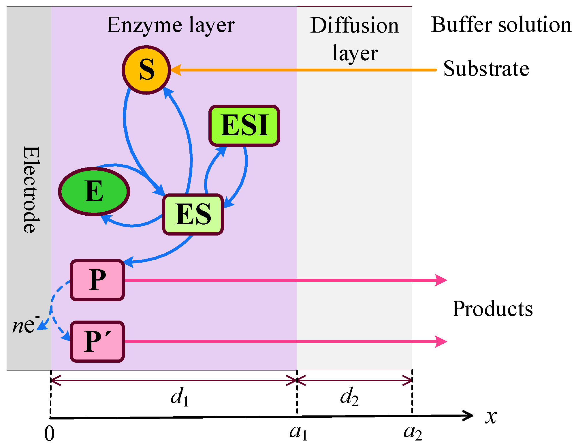
Figure 2.
Dynamics of the output current at ten values of the normalized substrate concentration , as indicated on the curves, with fixed parameters = , = , and , in IA (a) and BA (b) modes. Other parameters are defined in (16).
Figure 2.
Dynamics of the output current at ten values of the normalized substrate concentration , as indicated on the curves, with fixed parameters = , = , and , in IA (a) and BA (b) modes. Other parameters are defined in (16).
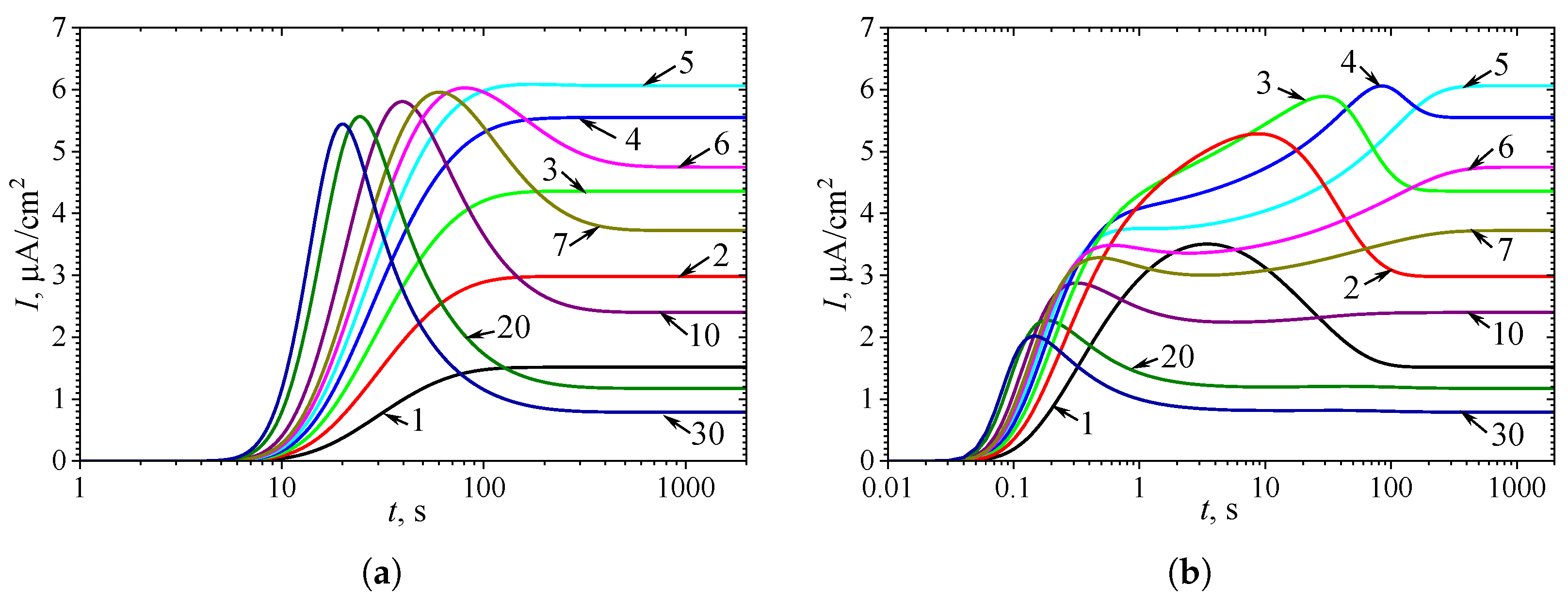
Figure 3.
Number of extrema of the output current vs. the diffusion module and the normalized substrate concentration , with fixed parameters = and , for IA (a) mode and BA (b) mode. Other parameters are defined in (16). The yellow line is defined in (17).
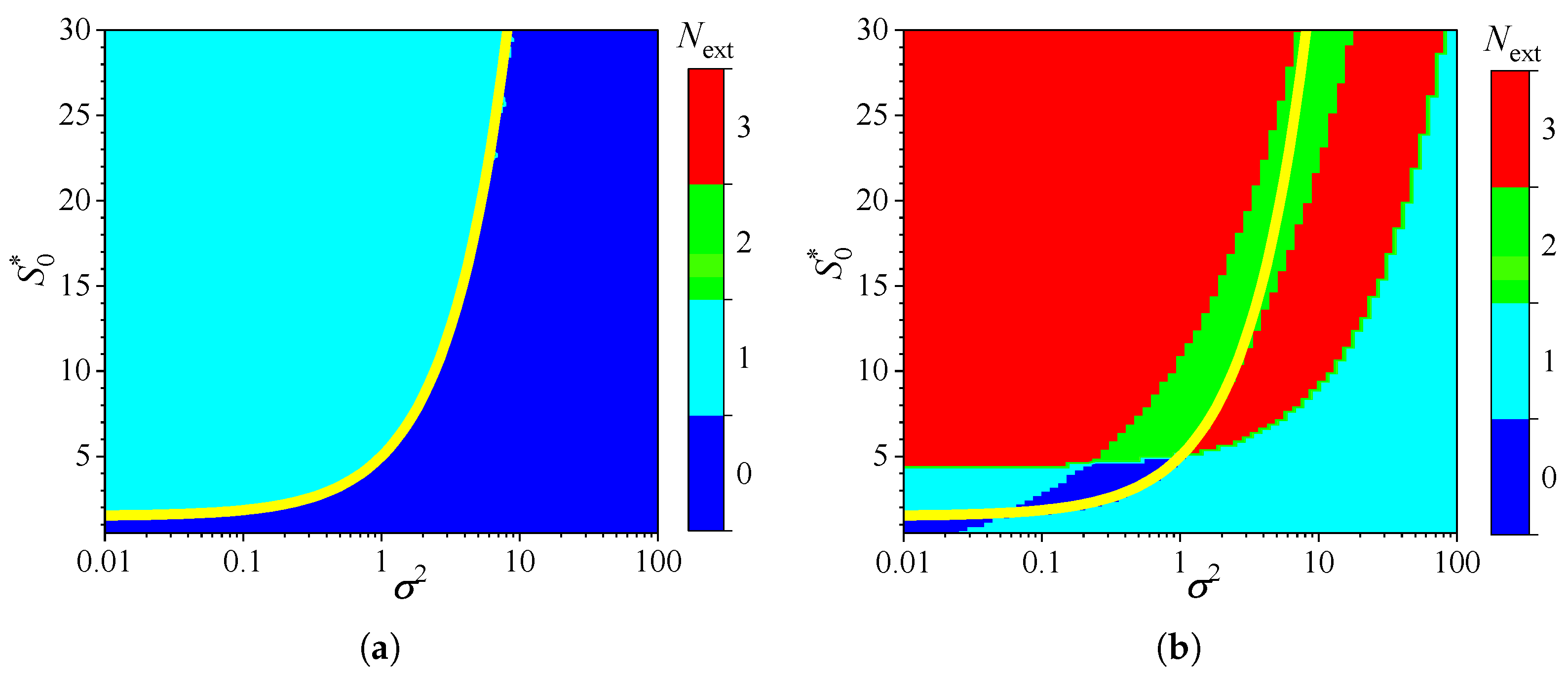
Figure 4.
Dynamics of the output current at ten values of the diffusion module , as indicated on the curves, with a fixed substrate concentration = 10, in IA (a) mode and BA (b) mode. Other parameters are the same as in Figure 3.
Figure 4.
Dynamics of the output current at ten values of the diffusion module , as indicated on the curves, with a fixed substrate concentration = 10, in IA (a) mode and BA (b) mode. Other parameters are the same as in Figure 3.
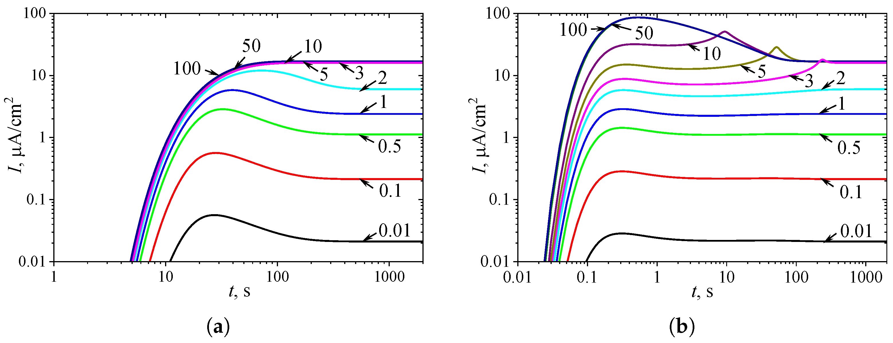
Figure 5.
Number of extrema of the biosensor current vs. the Biot number and the normalized substrate concentration , with fixed parameters = , and , for IA (a) mode and BA (b) mode. Other parameters are defined in (16). The yellow line is defined in (18).
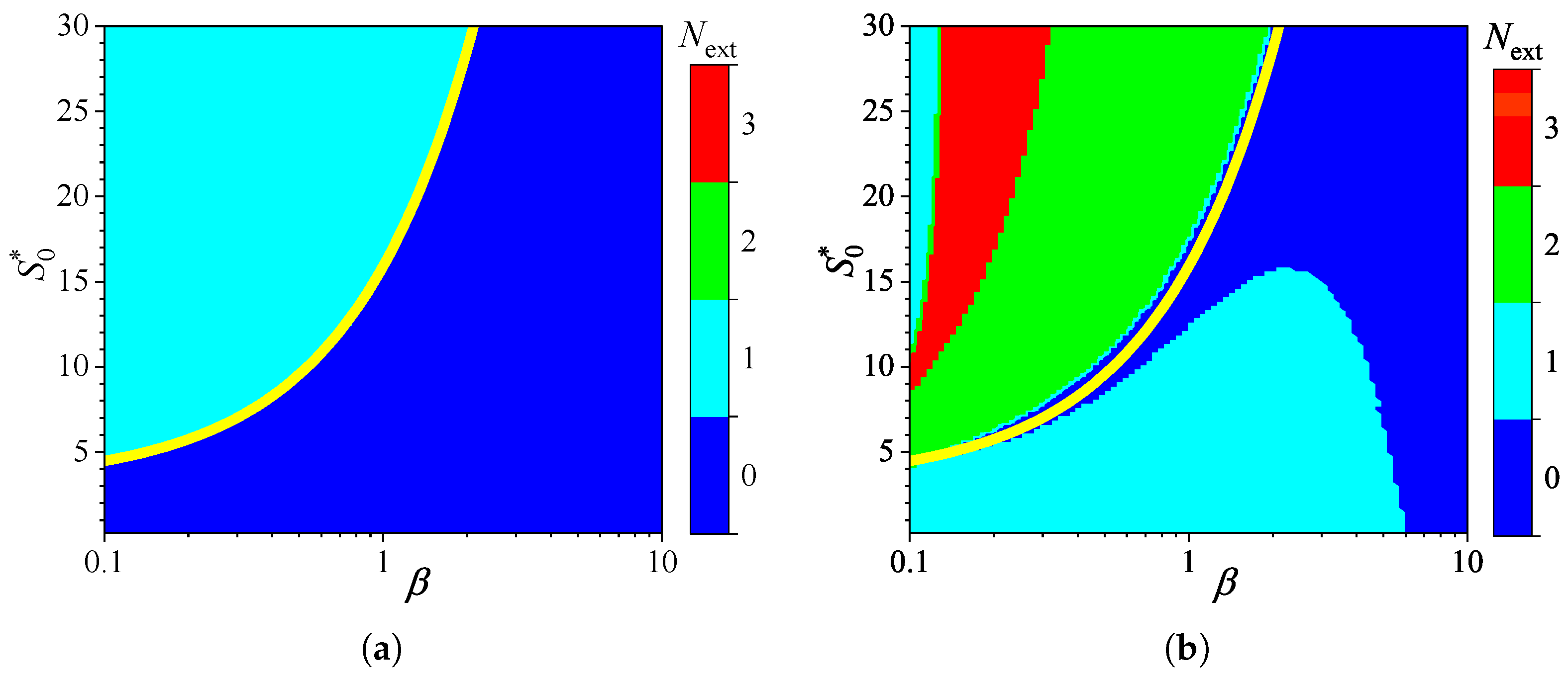
Figure 6.
Dynamics of the output current at nine values of the Biot number , as indicated on the curves, with with a fixed substrate concentration = 10, in IA (a) mode and BA (b) mode. Other parameters are the same as in Figure 5.
Figure 6.
Dynamics of the output current at nine values of the Biot number , as indicated on the curves, with with a fixed substrate concentration = 10, in IA (a) mode and BA (b) mode. Other parameters are the same as in Figure 5.
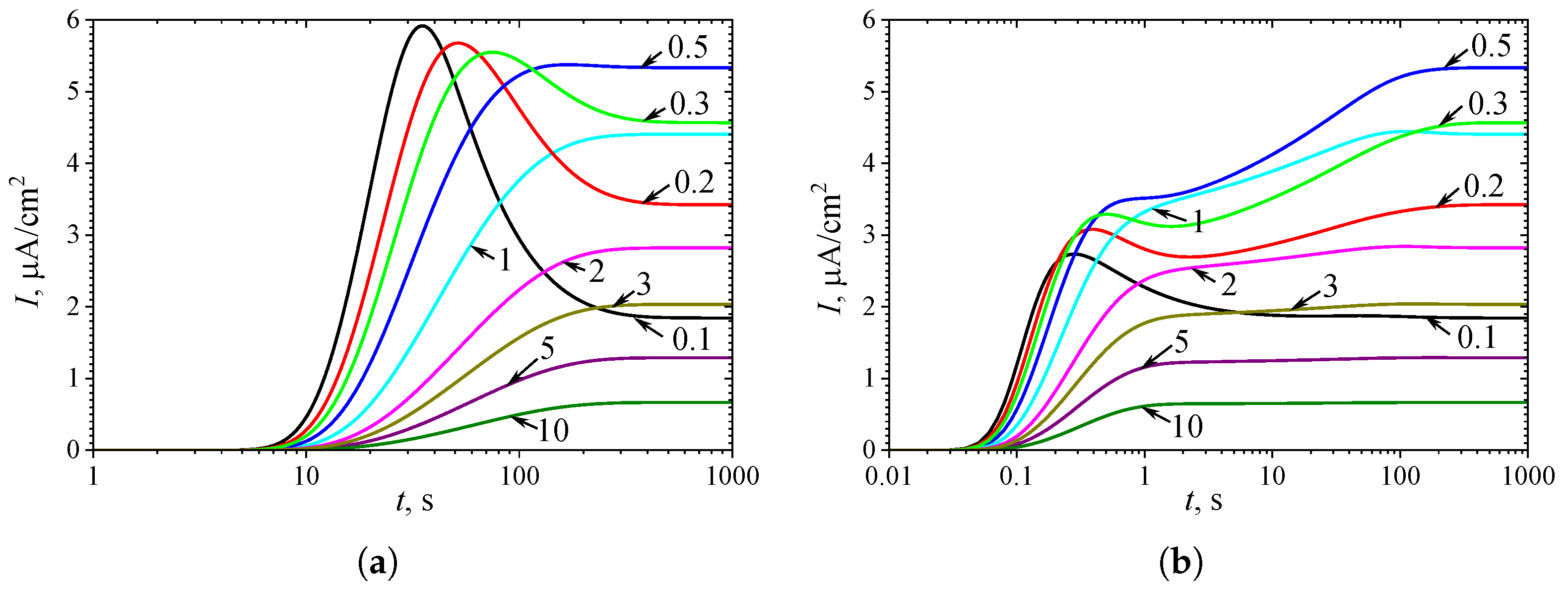
Figure 7.
Number of extrema of the biosensor current vs. the normalized inhibition constant and the normalized substrate concentration , with fixed parameters = , and , for IA (a) mode and BA (b) mode. Other parameters are defined in (16).
Figure 7.
Number of extrema of the biosensor current vs. the normalized inhibition constant and the normalized substrate concentration , with fixed parameters = , and , for IA (a) mode and BA (b) mode. Other parameters are defined in (16).
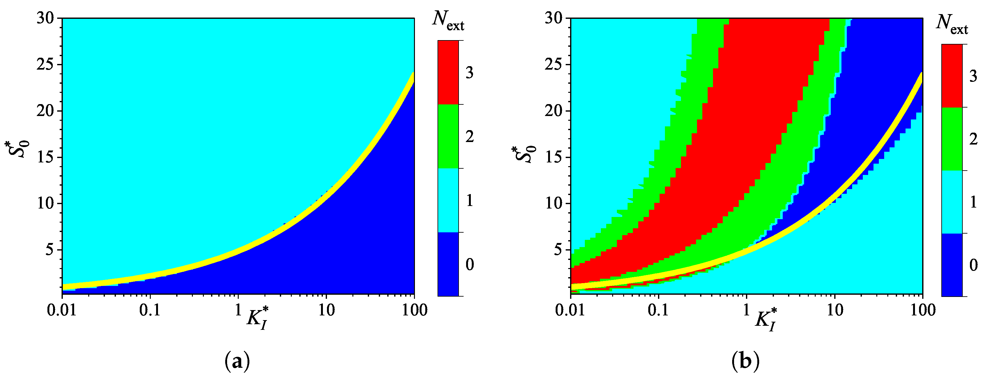
Figure 8.
Dynamics of the output current at eleven values of normalized inhibition constant , as indicated on the curves, with with a fixed substrate concentration = 10, in IA (a) mode and BA (b) mode. Other parameters are the same as in Figure 7.
Figure 8.
Dynamics of the output current at eleven values of normalized inhibition constant , as indicated on the curves, with with a fixed substrate concentration = 10, in IA (a) mode and BA (b) mode. Other parameters are the same as in Figure 7.

Disclaimer/Publisher’s Note: The statements, opinions and data contained in all publications are solely those of the individual author(s) and contributor(s) and not of MDPI and/or the editor(s). MDPI and/or the editor(s) disclaim responsibility for any injury to people or property resulting from any ideas, methods, instructions or products referred to in the content. |
© 2025 by the authors. Licensee MDPI, Basel, Switzerland. This article is an open access article distributed under the terms and conditions of the Creative Commons Attribution (CC BY) license (http://creativecommons.org/licenses/by/4.0/).
Copyright: This open access article is published under a Creative Commons CC BY 4.0 license, which permit the free download, distribution, and reuse, provided that the author and preprint are cited in any reuse.


