Practical Identification of Heat Exchanger Model Parameters

1. Introduction

State and parameter estimation are required for dynamic process modeling, monitoring, control and diagnostics in various fields, including petrochemicals, oil refining, paper production, electric power and aerospace industries, etc. The construction of such models is based on a powerful apparatus of ordinary differential equations (ODE). To solve practical problems, in addition to the direct problem, it is often necessary to determine the parameters of ODE systems (inverse Cauchy problem) from experimental data.

Many studies have been conducted to develop different approaches to achieve high quality estimation of the state and parameters. Among them, their simultaneous estimation has received increased attention due to its ability to achieve better stability and reliability of estimation. In its framework, the observed vector of states is extended by including the model parameters to be estimated [1,2,3], which makes it possible to estimate the states and parameters simultaneously. In the future, the well-developed apparatus of Kalman filtering can be applied to the problem thus extended [4,5,6,7].

However, in this case it is necessary that the formed extended system be completely observable. Methods of sensitivity analysis, global [8,9] and local [10,11], of observed variables to the estimated parameters, allow establishing the fact of identifiability [12,13] of these parameters. However, a situation is possible in which the corresponding matrix has full rank but is poor conditioned, which leads to additional problems associated with the fact that the solution to the problem may be sensitive to noise in the experimental data. To overcome the problems that arise, it is possible to use regularization methods [11,14], in particular, by selecting a set of estimated parameters [6,7,10,11], which allows improving the regular properties of the problem and ensuring the required quality of estimation.

2. Materials and Methods

The object of study was a counter-current heat exchanger model described by a system of ordinary nonlinear differential equations [15]. In conditions of incomplete measurement of states and parameters, their simultaneous estimation is difficult due to poor conditionality of the problem, which leads to the need to apply regularization measures. In the work, a selection of a set of estimated parameters for identification is made in relation to experimental data obtained as a result of studying the model in the Unisim Design software environment. The use of orthogonalization and optimization methods made it possible to select the estimated parameters, the effectiveness of which was confirmed by statistical modeling of the sigma-point filtering algorithm [5,16], for the model under study.

The object described by a system of nonlinear finite-difference equations:

$$\begin{gathered} x\left(k+1\right)=f\left(x\left(k\right),\theta ,k\right),k\in \left(0,T\right), \\ x\left(0\right)=x_{0,} \\ y\left(k\right)=h\left(x\left(k\right),\theta ,k\right), \end{gathered}$$

(1)

where $x\left(k\right)\in R^{n_x}$ - vector of state functions ($n_x$- number of equations, $\theta \in R^{n_{\theta }}$ – vector of parameters ($n_{\theta }$- number of parameters), $y\left(k\right)\in R^{n_y}$- vector of measurement functions,$f\left(·\right)$ and $h\left(·\right)$ - equations of state and measurement, generally nonlinear ($n_y\le n_x$), respectively.

2.1. Extended System

To estimate the state and parameters of system (1) simultaneously, we consider extending the vector of states by including a parameter, which is a standard approach to estimate the state and parameters simultaneously [12,13]. We can then obtain the following extended system

$$x_{\theta }\left(k+1\right)=\left[\begin{array}{c}f\left(x\left(k\right),u\left(k\right),\theta \left(k\right)\right)\\ \theta \left(k\right)\end{array}\right]=F_{\theta }\left(x_{\theta }\left(k\right),u\left(k\right)\right)$$

(2a)

$$y\left(k\right)=H\left(x\left(k\right),\theta \left(k\right)\right)=H_{\theta }\left(x_{\theta }\left(k\right)\right)$$

(2b)

where $x_{\theta }\left(k\right)={\left[x{\left(k\right)}^T\theta {\left(k\right)}^T\right]}^T\in R^{n_x+n_{\theta }}$ – extended vector of states, $F_{\theta }\left(·\right)$and $H_{\theta }\left(·\right)$ - extended state and output equations, respectively.

The goal of simultaneous state and parameter estimation is now to estimate the extended state $x_{\theta }$ based on input and output information. First, we need to check whether the entire extended vector of states $x_{\theta }$ is observable. As shown in [7,10,14], we can check the rank of the sensitivity matrix computed along a typical trajectory within a sliding window of data of the extended system

$$S_{\theta }\left(k\right)=\left[\begin{array}{c}{S}_{y,x_{\theta }\left(k-N\right)}\left(k-N\right)\\ S_{y,x_{\theta }\left(k-N\right)}\left(k-N+1\right)\\ \begin{array}{c}⋮\\ S_{y,x_{\theta }\left(k-N\right)}\left(k\right)\end{array}\end{array}\right]$$

(3)

where N — the data window size must be no less than $n_x+n_{\theta }$.

The input sensitivities of the measured vector in relation to the extended vector of states included in expression (3) based on the input and output data of the processes can be defined as [7,10,14]:

$$\begin{gathered} S_{y,x_{\theta }\left(k-N\right)}\left(i\right)={\displaystyle \frac{\partial H_{\theta }}{\partial x_{\theta }}}\left(i\right){\displaystyle \frac{\partial F_{\theta }}{\partial x_{\theta }}}\left(i-1\right){\displaystyle \frac{\partial F_{\theta }}{\partial x_{\theta }}}\left(i-2\right)\dots {\displaystyle \frac{\partial F_{\theta }}{\partial x_{\theta }}}\left(k-N\right), \\ {\displaystyle \frac{\partial F_{\theta }}{\partial x_{\theta }}}\left(i\right)=\left[\begin{array}{cc}{\displaystyle \frac{\partial F_{\theta }}{\partial x}}\left(i\right)& {\displaystyle \frac{\partial F_{\theta }}{\partial \theta }}\\ 0& I_{n_{\theta }\times n_{\theta }}\end{array}\right],{\displaystyle \frac{\partial H_{\theta }}{\partial x_{\theta }}}\left(i\right)=\left[\begin{array}{cc}{\displaystyle \frac{\partial H}{\partial x}}\left(i\right)& {\displaystyle \frac{\partial H}{\partial \theta }}\end{array}\right]. \end{gathered}$$

(4)

Checking the rank of the sensitivity matrix $S_{\theta }\left(k\right)$ at each sampling moment allows concluding that the extended vector of states can be estimated locally using the input and output data. In the case of incomplete rank, not all of its elements can be estimated. However, the presence of a full rank sensitivity matrix does not guarantee observability, especially for complex systems. The estimation problem faces certain difficulties when the matrix is close to a matrix with insufficient rank. In this case, the problem is poor conditioned, and the resulting solution is very sensitive to noise contained in the data, which leads to deviations in the parameter estimates.

Introducing additional channels of output variable measurement can have a positive effect, but it is not always possible or justified. In such cases, regularization methods such as ridge regression [17], principal component analysis [18] and parameter selection are used [7,10,14,19,20].

2.2. Selecting Parameters

The procedures for selecting parameters for estimation must consider the extent to which small variations in parameters affect the output data, as well as the correlation between effects. If the effect of a change in a parameter on output variables is small by some standard, then it will be impossible to accurately estimate this parameter from such data. Similarly, if variations in two or more parameters result in the same effect on the output data, then these effects are correlated and such data are indistinguishable, i.e., it is impossible to estimate the values of these parameters unambiguously. In other words: no sensitivity vector corresponding to a parameter can be approximately expressed as a linear combination of other sensitivity vectors of the selected parameters.

Various selection methods based on these two rules have been developed, including the orthogonalization method [11,21], the collinearity index approach [22,23] the principal component-based method [24,25], the eigenvalue-based method [26,27], the relative gain array-based method [28], the hierarchical parameter clustering method, [29] and the hybrid methods. [30,31]. All methods consider two selection criteria simultaneously, but differ in how much weight is given to one criterion over the other, and in how parameter combinations are selected for estimation. All of these methods have been shown to be computationally inexpensive and to work well on the examples to which they have been applied, but none of these methods can guarantee the selection of an optimal set of parameters.

The selection of a set of parameters for estimation from the entire set of model parameters can be made on the basis of heuristic methods, as well as optimization methods. Thus, if the influence of a parameter on the output data of the model is insignificant, then its estimation will be ineffective, since even insignificant noise in measurements will have a significant effect on the estimation.

Based on sensitivity analysis, the main factors influencing the choice of parameters are: the norm of the sensitivity vector of the output data to the selected parameter must have a significant value compared to the norms of the sensitivity vectors for other parameters, and low correlation of the sensitivity vectors of the selected parameters.

2.2.1. Orthogonal Algorithm

Since output data and parameters usually have different units of measurement, and there may be order differences in their numerical values, sensitivity vectors are often normalized:

$${\displaystyle \frac{{\overline{\theta }}_i}{{\sigma }_j}}·s_j,i=1,\dots ,n_{\theta };j=1,\dots ,n_y,$$

(5)

where ${\overline{\theta }}_i$ – nominal value of the i-th parameter; ${\sigma }_j$- root mean square deviation of the j-th output variable.

Sequence of the algorithm [11,14,20,27].

Calculate the sum of the squares of the elements of each column$S_{\theta }$.

Select the parameter whose column in $S_{\theta }$ has the largest sum of squares of its elements as the first parameter to be estimated.

Mark the corresponding column as Xl (l=1 or the first iteration).

Calculate ${\widehat{s}}_l$, the prediction of the full sensitivity matrix $S_{\theta }$, using a subset of the columns Xl:

$${\widehat{s}}_l=X_l{\left(X_l^T{X}_l\right)}^{-1}{X}_l^T{S}_{\theta }.$$

(6)

Calculate the residual matrix Rl: Rl=$S_{\theta }$ -${\widehat{s}}_l$

Calculate the sum of the squares of the residuals in each column of Rl. The column with the largest sum corresponds to the next parameter to be estimated.

Select the appropriate column in $S_{\theta }$ and complete the matrix Xl, by including the new column. We denote the extended matrix as Xl+1.

Increment the iteration counter by one and repeat steps 4–7 until the sum of the squares of the elements of the largest column in the residual matrix is less than the specified threshold value.

Algorithm 2 of the orthogonal method [11,14,20,27,32].

1. Set the stopping criterion δ1, the array of numbers of identifiable parameters U = ∅ and the array of numbers of unidentifiable parameters $I=\left\{1,\dots ,n_{\theta }\right\}$. Construct the sensitivity matrix $S_{\theta }$ of the following form (2).

2. Select from the sensitivity matrix $S_{\theta }$ the column l with the largest sum of squares of the elements, add it to the matrix E as the first column and remove it from $S_{\theta }$. Add the element l to the array U and remove it from I.

3. If U is blank, then stop the algorithm: for this model, all parameters are identifiable. Otherwise, go to step 4.

4. For each column Sm, m = 1…n, of the matrix $S_{\theta }$, where n is the number of remaining columns from $S_{\theta }$, calculate the perpendiculars:

$$s_m^{\perp }=s_m-s_m^{proj},s_m^{proj}={{\displaystyle \sum }}_{i=1}^{n_{\theta }-n}{\displaystyle \frac{\left(s_m,E_i\right)}{\left(E_i,E_i\right)}}{E}_i,E=\left(E_1,\dots ,E_{n_{\theta }-n}\right),m=1,\dots ,n$$

(7)

5. From the obtained matrix of perpendiculars $S^{\perp }$ select the column l with the largest sum of squares of the elements. If $\Vert S_l^{\perp }\Vert \le \mathsf{\delta }$, then stop the algorithm. All parameters from U are identifiable, otherwise go to step 6.

6. Add element l to U, remove it from U, remove the corresponding column from $S_{\theta }$ and add it to E, go to step 3.

2.2.2. Optimization of the Identifiable Parameter’s Selection

Methods for selecting sets of estimated parameters [7,10,14,19,20] that allow solving the problem require a balance of such indicators as the magnitude of effects and the correlation between them, since the correctness of the choice cannot be guaranteed. A more systematic approach consists of formalizing the problem as an optimization. The matrix $S_{\theta }^T{S}_{\theta }$ and the Fisher information matrix depend on the same sensitivity vectors, and the matrix inverse to the Fisher information matrix provides a lower bound on the covariance matrix of the parameter estimates, according to the Rao-Kramer inequality (the covariance matrix of the observation noise scales the values and has no effect). Therefore, by purposefully synthesizing the sensitivity matrix (by selecting the estimated parameters), one can directly influence the accuracy of their estimation.

Let us formulate the problem using the D-criterion for planning experiments [33,34] in the following form:

$$\begin{gathered} J=\arg \underset{I}{\max }det\left(S_{\theta }^T{S}_{\theta }\right), \\ I=\left\{1,\dots ,n_{\theta }\right\}. \end{gathered}$$

(8)

It is noted [14] that if the sensitivity vector in the matrix ${\mathrm{S}}_{\mathsf{\theta }}$ has a small norm or it has vectors that are linearly dependent, then this leads to a small value of criterion (8), while the choice of estimated parameters that maximizes it creates the necessary conditions for improving the accuracy of the estimate.

3. Results

3.1. The Heat Exchanger Model

One of the key types of technological equipment for thermal power and oil refining plants are heat exchangers [15]. Due to the high inertia of the technological processes under consideration, the temperatures at the input to the heat exchangers change quite slowly relative to the residence time of the substance in the heat exchanger and the rate of change of the temperature of the heat exchanger partition, therefore most transient processes can be considered quasi-stationary. In this case, the temperature profile of the heat exchanger is close to the steady-state profile at the current input and output temperatures. Below is a model of a heat exchanger based on the assumption of a quasi-stationary process, as well as the assumption that the heat capacity of the substance changes slightly between the input and output of the heat exchanger.

Differential equations describing the weights of hot ($M_H$) and cold ($M_C$) substances in a heat exchanger (kg) depending on the flow rates of the input flows:

$${\displaystyle \frac{d{M}_H}{dt}}=F_H^{\left(0\right)}-F_H^{\left(1\right)},$$

(9)

$${\displaystyle \frac{d{M}_C}{dt}}=F_C^{\left(1\right)}-F_C^{\left(0\right)},$$

(10)

where $F_H^{\left(0\right)}$ and $F_C^{\left(1\right)}$ - input flow rates - hot and cold, respectively, kg/s; $F_H^{\left(1\right)}$ and $F_C^{\left(0\right)}$ - output flow rates - hot and cold, respectively, kg/s.

$${\displaystyle \frac{d{H}_H^{\left(1\right)}}{dt}}={\displaystyle \frac{F_H^{\left(0\right)}\left(H_H^{\left(0\right)}-H_H^{\left(1\right)}\right)-Q_H}{M_H}},$$

(11)

$${\displaystyle \frac{d{H}_C^{\left(0\right)}}{dt}}={\displaystyle \frac{F_C^{\left(1\right)}\left(H_C^{\left(1\right)}-H_C^{\left(0\right)}\right)+Q_C}{M_C}},$$

(12)

$H_H^{\left(1\right)}$ and $H_C^{\left(0\right)}$ - specific enthalpies of hot and cold substances in a heat exchanger, J/kg.

$Q_H$ and $Q_C$ – heat flows from a hot substance to a partition and from a partition to a cold substance, W.

Due to the assumption that the heat capacities of the substance change little between the input and output, expressions for the logarithmic mean temperature difference can be used for the heat flows:

$$Q_H=U_{H}A{\displaystyle \frac{\left(T_H^{\left(0\right)}-T_B^{\left(0\right)}\right)-\left(T_H^{\left(1\right)}-T_B^{\left(1\right)}\right)}{ln\frac{T_H^{\left(0\right)}-T_B^{\left(0\right)}}{T_H^{\left(1\right)}-T_B^{\left(1\right)}}}},$$

(13)

$$Q_{\text{С}}=U_{C}A{\displaystyle \frac{\left(T_B^{\left(0\right)}-T_C^{\left(0\right)}\right)-\left(T_B^{\left(1\right)}-T_C^{\left(1\right)}\right)}{ln\frac{T_B^{\left(0\right)}-T_C^{\left(0\right)}}{T_B^{\left(1\right)}-T_C^{\left(1\right)}}}},$$

(14)

$U_H$ and $U_C$- heat transfer coefficients from a hot substance to a partition and from a partition to a cold substance, W/m2*0С; А – heat exchange surface area, m2; $T_B^{\left(0\right)}$ and $T_B^{\left(1\right)}$- temperatures of the ends of the partition, 0С; $T_H^{\left(0\right)}$ and $T_C^{\left(1\right)}$- temperatures of hot and cold intput flows, 0С; $T_H^{\left(1\right)}$and $T_C^{\left(0\right)}$ - temperatures of hot and cold output flows, 0С.

Expressions for $T_B^{\left(0\right)}$ and $T_B^{\left(1\right)}$ have the following form:

$${\displaystyle \frac{d{T}_B^{\left(0\right)}}{dt}}={\displaystyle \frac{2}{M_B{C}_B}}\left[{\displaystyle \frac{\left(T_H^{\left(0\right)}-T_B^{\left(0\right)}\right)Q_H}{\left(T_H^{\left(0\right)}-T_B^{\left(0\right)}\right)+\left(T_H^{\left(1\right)}-T_B^{\left(1\right)}\right)}}-{\displaystyle \frac{\left(T_B^{\left(0\right)}-T_C^{\left(0\right)}\right)Q_C}{\left(T_B^{\left(0\right)}-T_C^{\left(0\right)}\right)+\left(T_B^{\left(1\right)}-T_C^{\left(1\right)}\right)}}\right],$$

(15)

$${\displaystyle \frac{d{T}_B^{\left(1\right)}}{dt}}={\displaystyle \frac{2}{M_B{C}_B}}\left[{\displaystyle \frac{\left(T_H^{\left(1\right)}-T_B^{\left(1\right)}\right)Q_H}{\left(T_H^{\left(0\right)}-T_B^{\left(0\right)}\right)+\left(T_H^{\left(1\right)}-T_B^{\left(1\right)}\right)}}-{\displaystyle \frac{\left(T_B^{\left(1\right)}-T_C^{\left(1\right)}\right)Q_C}{\left(T_B^{\left(0\right)}-T_C^{\left(0\right)}\right)+\left(T_B^{\left(1\right)}-T_C^{\left(1\right)}\right)}}\right],$$

where $M_B$ – partition weight, kg; $C_B$ – specific heat capacity of the partition material, J/kg*0С.

The relationships for the densities of hot ${\rho }_H^{\left(1\right)}$ and cold ${\rho }_C^{\left(0\right)}$ substances in the heat exchanger are determined in the form:

${\rho }_H^{\left(1\right)}={\displaystyle \frac{M_H}{V_H}},$ ${\rho }_C^{\left(0\right)}={\displaystyle \frac{M_C}{V_C}}$, kg/m3,

where $V_H$ and $V_C$ – volumes of spaces with hot and cold substances, m3.

Input flow consumptions

$$F_H^{\left(0\right)}=K_H\sqrt{{\rho }_H^{\left(0\right)}\left(P_H^{\left(0\right)}-P_H^{\left(1\right)}\right)},F_C^{\left(1\right)}=K_C\sqrt{{\rho }_C^{\left(1\right)}\left(P_C^{\left(1\right)}-P_C^{\left(0\right)}\right)},$$

(16)

where $K_H$ and $K_{\text{С}}$ - coefficients of hydraulic conductivity of hot and cold spaces.

Relationships between thermodynamic parameters:

For input flow densities$\tilde{\rho }\left(T_C^{\left(1\right)},P_C^{\left(1\right)}\right)$, kg/m3;

for input flow pressures $P_H^{\left(1\right)}=\tilde{P}\left({\rho }_H^{\left(1\right)},H_H^{\left(1\right)}\right),P_C^{\left(0\right)}=\tilde{P}\left({\rho }_C^{\left(0\right)},H_C^{\left(0\right)}\right)$, Pa;

for specific enthalpies of hot $H_H^{\left(0\right)}=\tilde{H}\left(T_H^{\left(0\right)},P_H^{\left(0\right)}\right),$and cold $H_C^{\left(1\right)}=\tilde{H}\left(T_C^{\left(1\right)},P_C^{\left(1\right)}\right)$ substances, J/kg;

for output flow temperatures $T_H^{\left(1\right)},T_C^{\left(0\right)}$are determined from the equation of state of the substance or are given in tabular form:

$$\tilde{\rho }\left(T_C^{\left(1\right)},P_C^{\left(1\right)}\right), \tilde{P}\left({\rho }_H^{\left(1\right)},H_H^{\left(1\right)}\right),\tilde{H}\left(T_H^{\left(0\right)},P_H^{\left(0\right)}\right),\tilde{T}\left({\rho }_C^{\left(0\right)},H_C^{\left(0\right)}\right).$$

(17)

Let’s introduce state variables:

$x_1\left(k\right),x_2\left(k\right)-$ specific enthalpies of hot and cold substances in a heat exchanger; $x_3\left(k\right),x_4\left(k\right)-$ weights of hot and cold substances in the heat exchanger; $x_5\left(k\right),x_6\left(k\right)-$ temperatures of the ends of the partition.

Let us designate the parameters of the model to be estimated:

${\theta }_1\left(k\right),{\theta }_2\left(k\right)-$ heat transfer coefficients from a hot substance to a partition and from a partition to a cold substance, W/m 2*0С;

${\theta }_3\left(k\right)-$ partition weight, kg; ${\theta }_4\left(k\right),{\theta }_5\left(k\right)-$ coefficients of hydraulic conductivity of hot and cold spaces,${\displaystyle \frac{kg/s}{\sqrt{\frac{kg}{m^3}Pa}}}$.

Since the parameters of the model depend little on the technological process, we adopt

${\theta }_1\left(k\right)={\theta }_1\left(k+1\right)={\theta }_1,$

${\theta }_2\left(k\right)={\theta }_2\left(k+1\right)={\theta }_{2,}$

${\theta }_3\left(k\right)={\theta }_3\left(k+1\right)={\theta }_3,$

${\theta }_4\left(k\right)={\theta }_4\left(k+1\right)={\theta }_4,$

${\theta }_5\left(k\right)={\theta }_5\left(k+1\right)={\theta }_{5,},k=1,\dots .$

The following variables are available for measurement:

$y_2\left(k\right),y_4\left(k\right)-$ input and output flow temperatures, $T_H^{\left(1\right)}$- of hot and $T_C^{\left(0\right)}$- cold, 0С; $y_1\left(k\right),y_3\left(k\right)-$ pressure of input and output flows, $P_H^{\left(1\right)}$- of hot and $P_C^{\left(0\right)}$- cold, Pa.

Let us introduce the extended vector:

$$x_e\left(k\right)={\left(x_1\left(k\right)x_2\left(k\right)x_3\left(k\right)x_4\left(k\right)x_5\left(k\right)x_6\left(k\right){\theta }_1\left(k\right){\theta }_2\left(k\right){\theta }_3\left(k\right){\theta }_4\left(k\right){\theta }_5\left(k\right)\right)}^T,$$

(18)

Let’s present the heat exchanger model in these terms:

$$x_e\left(k\right)=f\left(x\left(k\right),\theta \left(k\right)\right),k=0,\dots$$

(19)

with initial conditions$x_e\left(0\right)=x_e\left(x\left(0\right),\theta \left(0\right)\right).$ The function includes differential equations (9)-(12), (15a), (15b) considering relations (13), (14).

The measurement model will take the following form:

$$y\left(k\right)=h\left(x\left(k\right),\theta \left(k\right)\right),k=0,\dots .$$

(20)

The function h(∙) is defined based on the Peng-Robinson equation of state [35,36,37] and allows one to determine the values of temperatures and pressures of flows for the specific enthalpies of matter and masses of substances calculated using model (19).

3.1.1. Modeling Results

The model of the counter-current one-dimensional heat exchanger was built in the Unisim Design software environment. Nitrogen was used as a heat carrier. The technological parameters of the simulated heat exchanger and the process parameters are given in Table 1

The experimental material represents the realizations of disturbances and output variables (Table 2) measured over 7200 seconds, with an interval of 1 s.

The task is to build a process model that includes 6 state variables and 5 parameters based on the results of the experiment in the Unisim Design environment, the conditions of its implementation (Table 1 and Table 2), as well as a table of thermodynamic properties of the coolant. At the same time, in conditions of the nonlinear nature of the interaction, the interdependence of technological factors, the presence of disturbances and the impossibility of measuring a number of indicators, it is necessary to resolve issues of local identifiability of the model parameters.

3.2. Selecting Parameters for Estimation

Let’s form a subset of estimated parameters using the orthogonal method. According to its algorithm, we will determine the column of the matrix $S_{\theta }$, that has the largest sum of squares of the elements. This is the 1st column, corresponding to the parameter ${\theta }_1$.

Next, according to the indicator of the norm of the projected sensitivity vector, which denotes the influence of parameters, in addition to the one already included, we select the next parameter ${\theta }_2$. Similarly, the parameters are included in the following order ${\theta }_4$,${\theta }_5$, ${\theta }_3$. Thus, a sequential selection of parameters is carried out by trial and error.

The application of the parameter selection optimization method yields the following results: the optimal solution in terms of criterion () yields a set that includes all parameters. Suboptimal options are located in the immediate vicinity of the solution found -${\theta }_1$, ${\theta }_2$,${\theta }_3$, ${\theta }_4$ and ${\theta }_2$, ${\theta }_3$,${\theta }_4$, ${\theta }_5$.

In order to determine the effect of the influence of the choice of the set of estimated parameters on the qualitative characteristics of the evaluation of the extended vector of states, including the above-defined variants of the sets - optimal and 2 suboptimal, we will carry out an estimation on the experimental material obtained during the modeling of the heat exchanger in the Unisim Design software environment. To estimate the extended state vector, the Sigma-Point Kalman Filter (Unscented) filtering algorithm was used, its relations are not given here and can be found in [5,16].

We will conduct experimental-statistical modeling using the Monte Carlo method. We will study the dependence on the variable initial conditions of the extended vector of states. In this case, we will assume that the vector of initial conditions is distributed according to the normal law:

$x_e^i\left(0\right)~N\left({\overline{x}}_e^i\left(0\right),{\sigma }_i^2\right),i=1,\dots ,11,$

where ${\overline{x}}_e^i\left(0\right)$- are equal to the corresponding parameters of the heat exchanger equipment for $i=1,\dots ,6$ and the parameters of the technological process for $i=7,\dots ,11$. The variances ${\sigma }_i^2$ are taken to be approximately 2,5% of ${\overline{x}}_e^i\left(0\right)$. The variance of the error of the Peng-Robinson equation in (20) is taken to be equal to 2.5% of the nominal.

For each variant, based on the generated initial conditions, an evaluation was performed using the sigma-point algorithm (Sigma-Point Kalman Filter (Unscented) filtering. The subsets of the identifiable parameters to be investigated, defined in Section 4.2, were included in the extended state vector (18). The simulation results of 20 realizations of each investigated variant were averaged and summarized in Table 3.

The results of the algorithm’s evaluation of the measured variables (20) for the optimal subset of the identified parameters and the same variables obtained in the Unisim Design programming environment are shown in Figure 1.

Figure 1. Averaged realizations of observed hot substance pressure fluctuations measured using the Unisim Design model and estimated using the Sigma-Point Kalman Filter (Unscented).

Figure 1. Averaged realizations of observed hot substance pressure fluctuations measured using the Unisim Design model and estimated using the Sigma-Point Kalman Filter (Unscented).

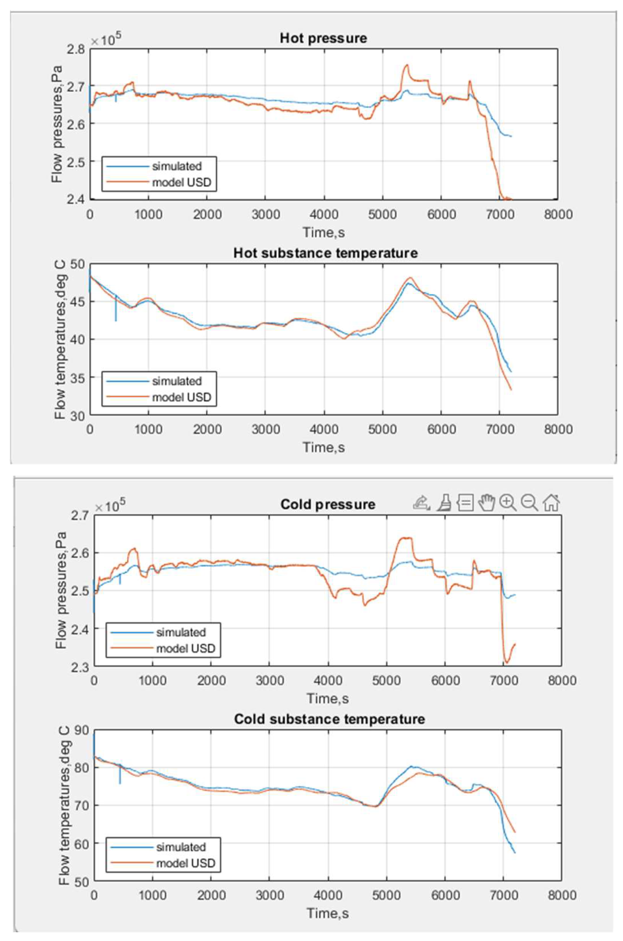
Figure 2. Autocorrelation functions of residual errors of parameter estimates.

Figure 2. Autocorrelation functions of residual errors of parameter estimates.

The correlation is small for all lags except 0. The average correlation is close to zero, and the correlation does not show any significant non-random variation. These characteristics increase confidence in the effectiveness of the model parameter estimation.

4. Conclusions

The problem of practical identification of a direct-flow heat exchanger model is investigated. The use of algorithms for simultaneous estimation of the state and parameters of the model leads to the need to study the problem of practical identifiability associated with incomplete measurement of output variables. Regularization methods associated with poor conditioning of the estimation problem are considered, the capabilities of algorithms for selecting a set of identifiable parameters are studied. To meet the requirements of low correlation of information about the parameters and high effect of their influence on the output variables, the methods of orthogonalization and optimization are applied to the experimental material obtained as a result of modeling the heat exchanger in the Unisim Design software environment. Illustrative materials of the results of applying the specified algorithms for selecting the identified parameters of the model using the sigma-point filtering algorithm are provided.

References

- Valluru, J; Patwardhan, S.C. An Integrated Frequent RTO and Adaptive Nonlinear MPC Scheme Based on Simultaneous Bayesian State and Parameter Estimation. Industrial & Engineering Chemistry Research, 2019, 58(18), pp. 7561-7578. [CrossRef]
- Kamalapurkar, R. Simultaneous state and parameter estimation for second-order nonlinear systems. In Proceedings of the 2017 IEEE 56th Annual Conference on Decision and Control (CDC), Melbourne, VIC, Australia, 12-15 December 2017; pp. 2164–2169. [Google Scholar] [CrossRef]
- Song, Bo.; Soumya, R.S.; Xunyuan, Y.; Jinfeng, L.; Sirish, L.S. Parameter and state estimation of one-dimensional infiltration processes: A simultaneous approach. Mathematics, 2020, 8(1), p.134, pp.1-22. [CrossRef]
- Kalman, R.E.; Bucy, R.S. New results in linear filtering and prediction theory. Journal of Basic Engineering, 1961, 83(1), pp. 95–108. [CrossRef]
- Grewal, M.S.; Andrews, A.P. Kalman Filtering: Theory and Practice Using MATLAB, 2nd ed.; John Wiley and Sons, Inc.: New York, USA, 2001; p. 397. [Google Scholar] [CrossRef]
- Stojanovic, V.; He, S.P.; Zhang, B.Y. State and parameter joint estimation of linear stochastic systems in presence of faults and non-Gaussian noises. International Journal of Robust and Nonlinear Control, 2020, 30(16), pp. 6683-6700. [CrossRef]
- Liu, S.Y.; Ding, F.; Hayat, T. Moving data window gradient-based iterative algorithm of combined parameter and state estimation for bilinear systems. International Journal of Robust and Nonlinear Control, 2020, 30(6), pp. 2413-2429. [CrossRef]
- Sobol’, I.M. Global sensitivity indices for nonlinear mathematical models and their Monte Carlo estimates. Mathematics and Computers in Simulation, 2001, Vol.55., Issues 1-3, pp. 271– 280. [CrossRef]
- Saltelli, A.; Annoni, P. How to avoid a perfunctory sensitivity analysis. Environmental Modelling & Software, 2010, 25(12), pp. 1508– 1517. [CrossRef]
- Liu, J.B.; Gnanasekar, A.; Zhang, Y.; et al. Simultaneous state and parameter estimation: the role of sensitivity analysis. Industrial & Engineering Chemistry Research, 2021, 60(7), pp. 2971-2982. [CrossRef]
- Yao, K.Z.; Benjamin, M.Sh.; Bo, K.; McAuley, K.; Bacon, D.W. Modeling Ethylene/Butene Copolymerization with Multi-site Catalysts: Parameter Estimability and Experimental Design. Polymer reaction engineering, 2003, 11(3), pp. 563–588. [CrossRef]
- Bellman, R.; Åström K.J. On structural Identifiability. Mathematical Biosciences, 1970, Vol.7., Issues 3-4, pp. 329–339. [CrossRef]
- Ljung, L.; Glad, T. On global identifiability for arbitrary model parametrizations. Automatica, Pergamon Press, Inc.: New York, USA, 1994, 30(2), pp. 265–276. [CrossRef]
- Kravaris, C.; Hahn, J.; Chu, Y.F. Advances and selected recent developments in state and parameter estimation. Computers & Chemical Engineering, 2013, 51(5), pp. 111-123. [CrossRef]
- Tasanbayev, S.; Uskenbayeva, G.; Kulniyazova, K.; Slastenov, I. Simultaneous estimation of states and parameters of a heat exchanger model using an extended Kalman filter. Bulletin of KazATC, 2023, 6(129), pp.111-120. [CrossRef]
- Semushin, I.V. Computational methods of algebra and estimation. Study guide, UlSTU, Inc.: Ulyanovsk, Russia, 2011; p. 366. ISBN 978-5-9795-0902-0.
- Box, G. E.; Draper, N. R. Response surfaces, mixtures, and ridge analyses, 2nd ed.; John Wiley and Sons, Inc.: New York, USA, 2006; p. 880. [Google Scholar] [CrossRef]
- Jolliffe, I.T. Principal component analysis, 2nd ed.; Springer-Verglar: New-York, USA, 2002; p. 488. [Google Scholar] [CrossRef]
- Miller, A. J. Subset selection in regression, 2nd ed.; CRC: New-York, USA, 2002; p. 256. [Google Scholar] [CrossRef]
- Krivorotko, O.I.; Andornaya, D.V.; Kabanikhin, S.I. Sensitivity analysis and practical identifiability of mathematical models of biology, Journal of Applied and Industr. Math., 2020, Vol.14, pp.115–130. [CrossRef]
- Lund, B.F.; Foss, B.A. Parameter ranking by orthogonalization - Applied to nonlinear mechanistic models, Automatica, 2008, 44(1), pp. 278-281. [CrossRef]
- Brun, R.; Reichert, P.; Kunsch, H.R. Practical identifiability analysis of large environmental simulation models, Water Resources Research., 2001; 37(4), pp. 1015-1030. [CrossRef]
- Omlin, M.; Brun, R.; Reichert P. Biogeochemical model of Lake Zurich: sensitivity, identifiability and uncertainty analysis, Ecological Modelling, 2001; 141(1-3), pp. 77-103. [CrossRef]
- Turanyi, T.; Nagy, T. Reduction of very large reaction mechanisms using methods based on simulation error minimization, Combustion and Flame., 2009; 156(2), pp. 417-428. [CrossRef]
- Degenring, D.; Froemel, C.; Dikta G.; Takors R. Sensitivity analysis for the reduction of complex metabolism models, J Process Control, 2004, 14(7), pp. 729-745. [CrossRef]
- Schittkowski, K. Experimental design tools for ordinary and algebraic differential equations, Ind Eng. Chem Res, 2007, 46(26), pp. 9137-9147. [CrossRef]
- Quaiser, T.; Monningmann, M. Systematic identifiability testing for unambiguous mechanistic modeling - application to JAK-STAT, MAP kinase, and NF-kappa B signaling pathway models. BMC Systems Biology, 2009, 3(50), pp. 1-21. [CrossRef]
- Sandink, C.A.; McAuley, K.B.; McLellan, P.J. Selection of parameters for updating in on-line models, Ind Eng Chem Res., 2001, 40(18), pp. 3936-3950. [CrossRef]
- Chu, Y.F.; Hahn, J. Parameter Set Selection via Clustering of Parameters into Pairwise Indistinguishable Groups of Parameters, Ind Eng Chem Res., 2009, 48(13), pp. 6000-6009. [CrossRef]
- Li, R.J.; Henson, M.A.; Kurtz, M.J. Selection of model parameters for off-line parameter estimation, IEEE Trans Control Syst Technol, 2004, 12(3), pp. 402-412. [CrossRef]
- Sun, C.L.; Hahn, J. Parameter reduction for stable dynamical systems based on Hankel singular values and sensitivity analysis, Chem Eng Sci., 2006, 61(16), pp. 5393-5403. [CrossRef]
- Latyshenko, V.; Krivorotko, O.; Kabanikhin, S.; Zhang, Sh.; Kashtanova, V.; Yermolenko, D. Identifiability analysis of inverse problems in biology, In Proceedings of the 2nd International Conference on Computational Modeling, Simulation, and Applied Mathematics (CMSAM-2017), Beijing, China, October 22-23, 2017, pp. 567–571. [CrossRef]
- Franceschini, G.; Macchietto, S. Model-based design of experiments for parameter precision: State of the art, Chem Eng Sci., 2008, 63(19), pp. 4846-4872. [CrossRef]
- Miao, H.Y.; Xia, X.H.; Perelson, A.S.; Wu, H.L. On identifiability of nonlinear ODE models and applications in viral dynamics, SIAM Review, 2011, 53(1), pp. 3-39. [CrossRef]
- Haghtalab, A.; Mahmoodi, P, Mazloumi, S.H. A modified Peng–Robinson equation of state for phase equilibrium calculation of liquefied, synthetic natural gas, and gas condensate mixtures, The Canadian Journal of Chemical Engineering, 2011, 89(6), pp. 1376-1387. [CrossRef]
- Peng, D.Y.; Robinson, D.B. A new two-constant equation of state, Ind. Eng. Chem. Fundam., 1976, 15(1), pp. 59–64. [CrossRef]
- Peng D.Y., Robinson D.B. Two and three phase equilibrium calculations for systems containing water, The Canadian Journal of Chemical Engineering, 1976, 54(5), pp.595–599. [CrossRef]