
Submitted:
15 July 2025
Posted:
15 July 2025
You are already at the latest version
Abstract
The various forms of Airy’s differential equation are discussed in this work together with the special functions that arise in the processes of their solutions. Further properties of the arising integral functions are discussed and their connections to existing special functions are derived. A generalized form of the Scorer function is obtained and expressed in terms of the generalized Airy’s and Nield-Kuznetsov functions. Complementary functions to the Nield-Kuznetsov functions are discussed, and higher derivatives of all generalized functions arising in this work are obtained together with their associated generalized Airy’s polynomials. A computational procedure for the generalized Scorer function is introduced and applied to computing and graphing it for different values of its index. Solution of an initial value problem involving the generalized Scorer function is obtained.
Keywords:
Inhomogeneous Airy’s equation
; Generalized Scorer function
; Generalized Airy’s polynomials
; Nield-Kuznetsov functions
1. Introduction
Airy’s differential equation and its associated Airy’s functions date back to the nineteenth century, [1]. They are as relevant today as they were then due to their many applications in mathematical physics, optics, electromagnetism and fluid dynamic modeling, among other fields of endeavour (cf. [2,3,4] and the references therein). A large number of differential equations in quantum theory can be reduced to Airy’s equation by an appropriate change of variables, thus adding to the importance and relevance of studies of Airy’s functions and other related special functions, [3,4].
Although Airy’s equation has been largely studied in its homogeneous form, it is considered in this work in the following inhomogeneous form, suggested by Miller and Mursi [5], wherein is a continuous function of the non-negative, real variable , and prime notation denotes ordinary differentiation with respect to the independent variable:
When , general solution to Equation (1) can be expressed in the form:
where are arbitrary constants, and and are Airy’s functions of the first- and second-kind, respectively, [2].
When , Scorer [6] obtained the following general solutions using variation of parameters. For , general solution to Equation (1) is given by:
and when , general solution is given by:
where are arbitrary constants.
The functions and are known as the Scorer functions, [2,4], or the inhomogeneous Airy’s functions, and arise in Raman scattering in chemical physics and in some engineering applications, [7,8]. The Scorer functions are related to Airy’s functions by:
When , where is any constant, general solution to Equation (1) has been obtained in the following form, [9,10]:
where and are arbitrary constants, and is defined by:
The function was introduced by Nield and Kuznetsov [10] in their analysis of flow in the transition layer where the governing Brinkman’s equation was reduced to the inhomogeneous Airy’s equation by a special choice of the permeability function. The function is referred to as the standard Nield-Kuznetsov function of the first-kind, and its main properties were studied by Hamdan and Kamel [9], including the following relationships between and :
Using (10) and (11) in (3) and (4), respectively, it is easily seen that solutions (3) and (8) are equivalent when , while solutions (4) and (8) are equivalent when
In an attempt to offer modelling flexibility in the study of flow through the transition layer, Abu Zaytoon and Hamdan [11] introduced a permeability model that reduced Brinkman’s equation to the following generalized inhomogeneous Airy’s equation of integer index :
The homogeneous part of (12), that is when , was studied by Swanson and Headley [12] who expressed its general solution as:
wherein and are arbitrary constants, and the functions and are the generalized Airy’s functions of the first- and second-kind, respectively, defined as:
where , , and is the gamma function. The Wronskian of and is given by:
and the terms are the modified Bessel functions defined by the following formulas in which :
It should be noted that when the index in Equations (12)–(15), Airy’s equation and its solutions are recovered, although subscript is used instead of 1 for consistency with notation in the literature.
When , Abu Zaytoon and Hamdan [11] obtained and expressed the general solution to the inhomogeneous generalized Airy’s Equation (12) as:
where the function is the generalized Nield-Kuznetsov function of the first-kind, defined as:
Related to the Nield-Kuznetsov functions, , that arise and play a significant role in the solution to the inhomogeneous Airy’s equations, is the parametric Nield-Kuznetsov function of the first-kind, , with parameter a, which arises in the particular solution of the inhomogeneous Weber’s equation of the form:
General solution to (21) is expressed as:
where is defined by:
The functions are known as the Nield-Kuznetsov functions of the first kind. Their analysis and applications have been extensivley discussed and documented, [9,10,13], and include solution methodologies and methods of computations of the inhomogeneous Airy’s and Weber’s equations with initial and boundary conditions.
Recent work in this field includes the elegant work of Dunster, (cf. [14] and the references therein), on the Nield-Kuznetsov functions and the use of Laplace transform and uniform asymptotic expansions. Dunster [14] introduced the concept of a compelemtary function to the parametric Nield-Kuznetsov function and studied its convergence and its favourable properties, and discussed its role in the solution of (21).
Analysis of Airy’s polynomials that arise in higher derivatives of Airy’s functions has been carried out in the elaborate work of Abramochkin and Razueva, [15]. The same Airy’s polynomials, together with other polynomials, arise in the higher derivatives of and are important from both a theoretical and a practical point of view, as discussed by Hamdan et.al. [16].
Recent developments in the field include analysis of generalized forms of Airy’s equations due to either their associated applications or due to the arise of many interesting associated special functions. These include the work of Askari and Ansari (cf. [17] and the references therein) on higher-order differential equations and the Mainardi function, and the work of Cinque and Orsingher (cf. [18] and the references therein) on higher-order, Airy-type equations.
The recent work reported in [11,14,15,17,18], and the references therein, clearly represents an advancement of the state of knowledge in this field of Airy’s and generalized Airy’s equations, their solutions and applications. It motivate the current work in which we derive further properties and representations of these functions, and relate them to other special functions. In particular, specific objectives of the current work are as follows:
- Fill-in some knowledge gaps that exit in the available literature. To this end, the Scorer solutions to Equation (1), as given by Equations (3) and (4), are used to obtain solutions to Equation (1) when .
- Introduce complementary functions, albeit divergent, to and that might be of importance in asymptotic analysis.
- Provide representations of all special functions arising in this work in terms of modified Bessel functions.
- Advance the state of knowledge by introducing a generalized Scorer function, .
- Discuss higher derivatives of all generalized functions arising in this work and obtain their associated polynomials.
- Introduce a computational procedure for the newly introduced generalized Scorer function and applying it to computing and graphing the generalized Scorer function over a subinterval of the X-axis.
- Provide a solution to an initial value problem involving the generalized Scorer function.
In order to accomplish the above objectives, this work is organized as follows. In Section 2, solutions to Equation (1) when are expressed in terms of the Scorer functions and . The function is expressed in terms of the primitives of the Scorer functions, and its complement is derived. The Nield-Kuznetsov and Scorer functions are then expressed in terms of the modified Bessel functions.
In Section 3, the generalized Scorer function, , is derived and expressed it in terms of generalized Airy’s functions and the generalized Nield-Kuznetsov function . General solution to Equation (12) when is then derived and discussed. All generalized functions are expressed in terms of the modified Bessel functions, and a computational procedure for and is derived and applied to graphing for different values of . Solution to an initial value problem involving is obtained.
In Section 4, higher derivatives of all generalized functions appearing in this work are discussed, and generalizations of these derivatives are derived and expressed in terms of generalized Airy’s and other polynomials. Degrees of the resulting polynomials are and expressed in terms of the orders of the derivatives. Dependence of the polynomials on index , of the generalized Airy’s equation, is discussed.
A conclusion to the current work is provided to summarize the key findings, and to define a direction for future work.
2. Further Representations of Airy’s Related Special Functions
2.1. Solutions to Equation (1) when
Solutions to Equation (1) when are not readily available in terms of the Scorer functions. However, with the help of the Nield-Kuznetsov function and its connections to the Scorer functions the following proposition provides the form of solutions.
Proposition 1.
General solutions to the inhomogeneous Airy’s Equation (1) with
are given by:
Proof.
Substituting from (10) in (8), and from (11) in (8), yields (24) and (25), respectively. □
2.2. Relationship of to the Primatives of the Scorer Functions
In what follows, the relationships between and the Wronskians that involve Airy’s and Scorer’s functions are established. The following Wronskians have been reported in [4]:
Using (30)-(33) in (9) renders the following expressions for :
2.3. Bessel Function Representation of Airy’s, Scorer’s and the Nield-Kuznetsov Functions
Airy’s functions, their derivatives and integrals take the following forms in terms of the modified Bessel functions, [2,4], obtained from (14) and (15) with , , and
where the function is obtained from (17) and (18) as:
Using (36), (37), (40) and (41) in (9)-(11), the functions , and can be written in the following forms:
2.4. Complementary Function of
Aspnes [19,20] introduced a function that can be thought of as the complement of , and is defined by:
Dunster [14] introduced the concept of a complementary function to by extending its definition to , and discussed its convergence and favourable properties. This complement is defined by:
Now, defining , equations (23) and (47) give
Following the definition introduced by Dunster, [14], the complement of is defined as:
From (30) the integral is expressed as:
and using (50) in (49) yields:
Defining , the following expression is obtained:
Equation (52) can be written, with the help of the value as:
Both functions and , defined by Equations (51) and (53), respectively, involve a divergent integral, namely . However, they might be of value in future study of asymptotic behaviour and could serve as comparison functions of other improper integrals or infinite series.
3. Generalized Airy’s Inhomogeneous Equation
3.1. Generalized Airy’s and Nield-Kuznetsov Functions
Consider the generalized, inhomogeneous Airy’s Equation (12) in which is an integer and is a smooth function of its real, non-negative variable . Solution to the homogeneous part of this equation is given by (13), with the generalized Airy’s functions given by (14) and (15). The following derivatives of the functions and are obtained from Equations (14) and (15), respectively:
Integrals of the generalized Airy’s functions, obtained from (14) and (15), can be written as:
Upon using (14), (15), (20) and (54)-(57), the following expressions for and are obtained:
Complementary function to the generalized Nield-Kuznetsov function of the first-kind is defined by:
and the sum of and its complement is the function , defined by:
Again, both and involve the divergent integral , hence both are divergent.
3.2. Generalized Scorer Function
For the special cases of , general solutions to the inhomogeneous Airy’s equation (1) are expressed in terms of Airy’s and Scorer’s functions given by (6) and (7). When , the function satisfies equation (1) and when , then both and satisfy Airy’s inhomogeneous equation (1). In what follows, a generalized Scorer function , valid for , is introduced to satisfy the generalized Airy’s Equation (12) for any , including Define the generalized Scorer function in terms of the generalized Airy’s functions as:
in such a way that when , equation (6) is recovered. An expression for is provided by the following proposition.
Proposition 2.
The generalized Scorer function
is expressed in terms of
and
as:
Proof.
Equation (62) can be written as:
Using (20), Equation (64) takes the form:
The integral can be evaluated by applying formula 10.43.19 from DLMF( NIST), [21]. Using (14), takes the form:
Using the substitution , integral (66) takes the form:
Applying the following integral identity for the modified Bessel function of the second kind, valid for , namely:
with integral (67) takes the form:
Equation (69) reduces to the known value when and
Upon using (69) in (65), the expression for in (63) is obtained. □
With given by (63), general solution to Equation (12) can be obtained according to the following proposition.
Proposition 3.
General solution to the inhomogeneous generalized Airy’s Equation (12) when
is given by:
Proof.
Equation (63) provides the following expression for :
Using (70) in (19) yields:
Letting in (72), result (70) follows. □
It is worth noting that when , the general solution (72) becomes:
and when , the general solution (72) takes the form:
3.3. Bessel Function Representation of the Generalized Scorer Function
The generalized Scorer function, and its first derivative take the following forms, respectively, in terms of Bessel’s modified functions, obtained by substituting (15) and (59) in (63), then differentiating:
3.4. Values at of the Generalized Scorer Function and Its Derivative
The value is obtained from (63) as:
where and have been used. With the knowledge that for a non-integer p, , Equation (77) can be written as:
First derivative of is given by:
with value at zero given by:
wherein the values and have been used.
3.5. Computational Algorithm of the Generalized Functions
Following Swanson and Headley, [12], the generalized Airy’s functions are evaluated using the following relationships:
Based on the above, the generalized Nield-Kuznetsov function of the first-kind and the generalized Scorer function can be evaluated using the following expressions, obtained using (81)-(85) in (20) and (63), respectively:
where
For the sake of illustrating the above computational procedure, the generalized Scorer function is computed for the index values , over the interval , and plotted in Figure 1, which shows the possibility of turning points at values However, verification of turning points requires more extensive calculations using the above procedure. It should be noted that all computations were carried out using Maple.
3.6. Initial Value Problem Involving the Generalized Scorer Function
Consider the problem of solving Equation (12) with subject to the conditions: and , where and are real numbers. From general solution (74) and the given initial conditions, the following system of two equations in the two arbitrary constants and is obtained:
Solution of the above system of equations is given by:
Determination of values of and requires a knowledge of the values at zero of , , and , which are given by:
and and , which are given by (78) and (80), respectively. For the sake of illustration, computations have been carried using the values of . Once and are calculated, solution , as given by (74), is computed using the computational procedure of Section 3.5, above.
Solutions to the given initial value problem are shown in Figure 2, below, for
4. Higher Derivatives of
In a previous article, Hamdan et.al. [16] discussed higher derivatives of the Nield-Kuznetsov function and the polynomials arising from its derivatives. In what follows, expressions for higher derivatives of the generalized functions , , and are obtained.
4.1. Higher Derivatives of
Consider the homogeneous generalized Airy’s equation, written in the form
The following few higher derivatives are obtained by repeated differentiation of (96):
Each of the above derivatives of is expressed in terms of and , whose coefficients are polynomials. The generalized Airy’s functions, and satisfy Equation (96) and the derivatives above. The kth derivatives of and can thus be expressed in the following forms:
where is the polynomial coefficient of and of , and is the polynomial coefficient of and of in the kth derivative of and . A few of these polynomials are shown in the Table 1, below.
4.2. Higher Derivatives of
The inhomogeneous generalized Airy’s Equation (1), with , can be written as:
and the function satisfies the particular solution to the inhomogeneous generalized Airy’s Equation (104). We thus have:
The following few higher derivatives are obtained by repeated differentiation of (105):
Each of the above derivatives of is expressed in terms of and . The kth derivatives of is thus expressed in the following form:
where , and are the polynomial coefficients of , and the Wronskian , respectively, in the kth derivative of . A few of these polynomials are shown in the Table 1, below.
4.3. Higher Derivatives of
The generalized Scorer function is defined by Equation (67), which can be written in the form:
where is defined by Equation (88). The following few higher derivatives of are obtained by repeated differentiation of (112):
Each of the above derivatives of is expressed in terms of and . The kth derivatives of is thus expressed in the following form:
where , and are the polynomial coefficients of , and , respectively, in the kth derivative of . A few of these polynomials are shown in Table 1, below.
4.4. The Polynomial Coefficients and Iterative Definition of the Higher Derivatives
Polynomial coefficients , and obtained in the above higher derivatives are presented in Table 1. Degrees of the polynomials , and are shown in Table 2 and are expressed in terms of the order of the derivative, k, and the index, n, of the generalized Airy’s equation. These polynomials are needed to define higher derivatives iteratively, as discussed in what follows.
The k+1st derivatives of the generalized functions , , and take the following forms:
The polynomial coefficients , and , in the k+1st derivative are obtained from , and , in the kth derivative using the following relationships:
Equations (120)-(123) can thus be written in the following final forms that include the value of the Wronskian, , as given by Equation (16):
It is worth noting that the k+1st derivatives of the generalized Scorer function can be obtained in terms of the k+1st derivatives of and by differentiating (112) as follows:
Using (121) and (122) in (131) yields:
and using (124)-(126) in (132) gives:
4.5. Dependence of the Coefficient Polynomials on Index n
5. Conclusions
The main theme of this work has been the study and analysis of Airy’s and generalized Airy’s differential equations, and the integral functions that define their particular solutions. An attempt was made to fill in gaps that exit in the knowledge-base of the Nield-Kuznetsov and the Scorer functions. This includes defining the generalized Scorer function and studying some of its properties and its relationship to other special functions. A computational procedure was introduced for the generalized Scorer function and used in the solution of an initial value problem involving this function. Further properties of the Nield-Kuznetsov and the generalized Nield-Kuznetsov functions, and their relationships to the generalized Airy’s functions, have been discussed. All functions have been expressed in terms of modified Bessel functions. Furthermore, as higher derivatives of the Nield-Kuznetsov and Scorer functions give rise to important Airy’s polynomials and generalized Airy’s polynomials, iterative definitions of the higher derivatives together with iterative methods of generating these polynomials, have been introduced. While in this work the focus has been on the generalized Airy’s function with a constant forcing function, future directions in this work will consider non-linear, variable forcing functions.
Author Contributions
Authors contributed equally to this research from inception to calculations and writing, and reviewing of manuscript. Both authors have read and agreed to the published version of the manuscript.”
Funding
This research received no external funding
Data Availability Statement
Minor calculations are included. No additional data is available.
Acknowledgment
The authors wish to extend their sincere gratitude to the referees of this work. Their suggestions, recommendations, and constructive comments enhanced this work and resulted in elimination of errors.
Conflicts of Interest
The authors declare no conflicts of interest.
References
- Airy, G.B. On the intensity of light in the neighbourhood of a caustic. Trans. Cambridge Phil. Soc. 1838, 379–401. [Google Scholar]
- Abramowitz, M.; Stegun, I.A. Handbook of Mathematical Functions. Dover, New York,1984.
- Temme, N.M. Special Functions: An introduction to the Classical Functions of Mathematical Physics. John Wiley & Sons, New York, 1996.
- Vallée, O.; Soares, M. Airy Functions and Applications to Physics. World Scientific, London, 2004.
- Miller, J. C. P.; Mursi, Z. Notes on the Solution of the Equation . Quarterly J. Mech. Appl. Math., 3 (1950), pp. 113-118.
- Scorer, R.S. Numerical evaluation of integrals of the form and the tabulation of the function . Quarterly J. Mech. Appl. Math. 1950, 3, 107–112. [Google Scholar] [CrossRef]
- Gil, A.; Segura, J.; Temme, N.M. On non-oscillating integrals for computing inhomogeneous Airy functions. Math. Comput. 2001, 70, 1183–1194. [Google Scholar] [CrossRef]
- Lee, S.-Y. The inhomogeneous Airy functions, Gi(z) and Hi(z). J. Chem. Phys. 1980, 72, 332–336. [Google Scholar] [CrossRef]
- Hamdan, M.H.; Kamel, M.T. On the Ni(x) integral function and its application to the Airy’s non homogeneous equation Appl. Math. Comput. 2011, 21, 7349–7360. [Google Scholar]
- Nield, D.A.; Kuznetsov, A.V. The effect of a transition layer between a fluid and a porous medium: shear flow in a channel. Transp. Porous Med. 2009, 78, 477–487. [Google Scholar] [CrossRef]
- Abu Zaytoon, M. S.; Hamdan, M. H. On modeling laminar flow through variable permeability transition layer, Fluids 2025, 10(6), 151-168.
- Swanson, C. A.; Headley, V. B. An extension of Airy’s equation. SIAM J. Appl. Math. 1967, 15, 1400–1412. [Google Scholar] [CrossRef]
- Hamdan, M.H.; Alzahrani, S.M.; Abu Zaytoon, M.S.; Jayyousi Dajani, S. Inhomogeneous Airy’s and generalized Airy’s equations with initial and boundary conditions, Int. J. Circuits, Systems and Signal Processing 2021, 15, 1486–1496. [Google Scholar] [CrossRef]
- Dunster, T.M. Nield-Kuznetsov functions and Laplace transforms of parabolic cylinder functions. SIAM J. Math. Analysis 2021, 53, 5915–5947. [Google Scholar] [CrossRef]
- Abramochkin, E.G.; Razueva, E.V. Higher derivatives of Airy’s functions and of their products. SIGMA 2018, 14, 1–26. [Google Scholar]
- Hamdan, M.H.; Jayyousi Dajani, S.; Abu Zaytoon, M.S. Higher derivatives and polynomials of the standard Nield-Kuznetsov function of the first kind. Int. J. Circuits, Systems and Signal Processing 2021, 15, 1737–1743. [Google Scholar] [CrossRef]
- Askari, H.; Ansari, A. (2025),Stokes phenomenon for the M-wright function of order 1/n. Appl. Math. Comput. 2025, 487, 129088. [Google Scholar]
- Cinque, F.; Orsingher, E. General Airy-type equations, heat-type equations and pseudo-processes. 2025, J. Evol. Equ., 25, 17.
- Aspnes, D.E. (1966). Electric-field effects on optical absorption near thresholds in solids, Phys. Rev. 1966, 147, 554–566. [Google Scholar]
- Aspnes, D.E. Electric-field effects on the dielectric constant of solids, Phys. Rev. 1967, 153, 972–982. [Google Scholar]
- Olver, F.W.J.; Maximon, L.C. Chapter 10, Bessel Functions, Digital Library of Mathematical Functions, NIST, Version 1.2.4; Release date 2025-03-15. U.S. Department of Commerce.
Figure 1.
Graphs of for .
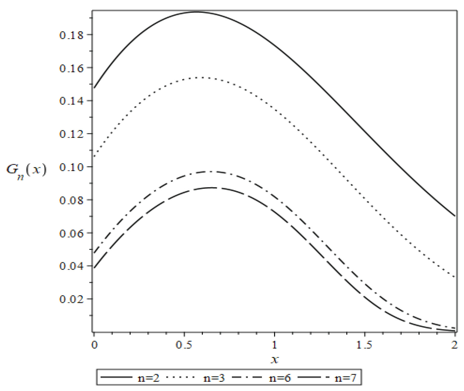
Figure 2.
Solution to the Initial Value Problem for .
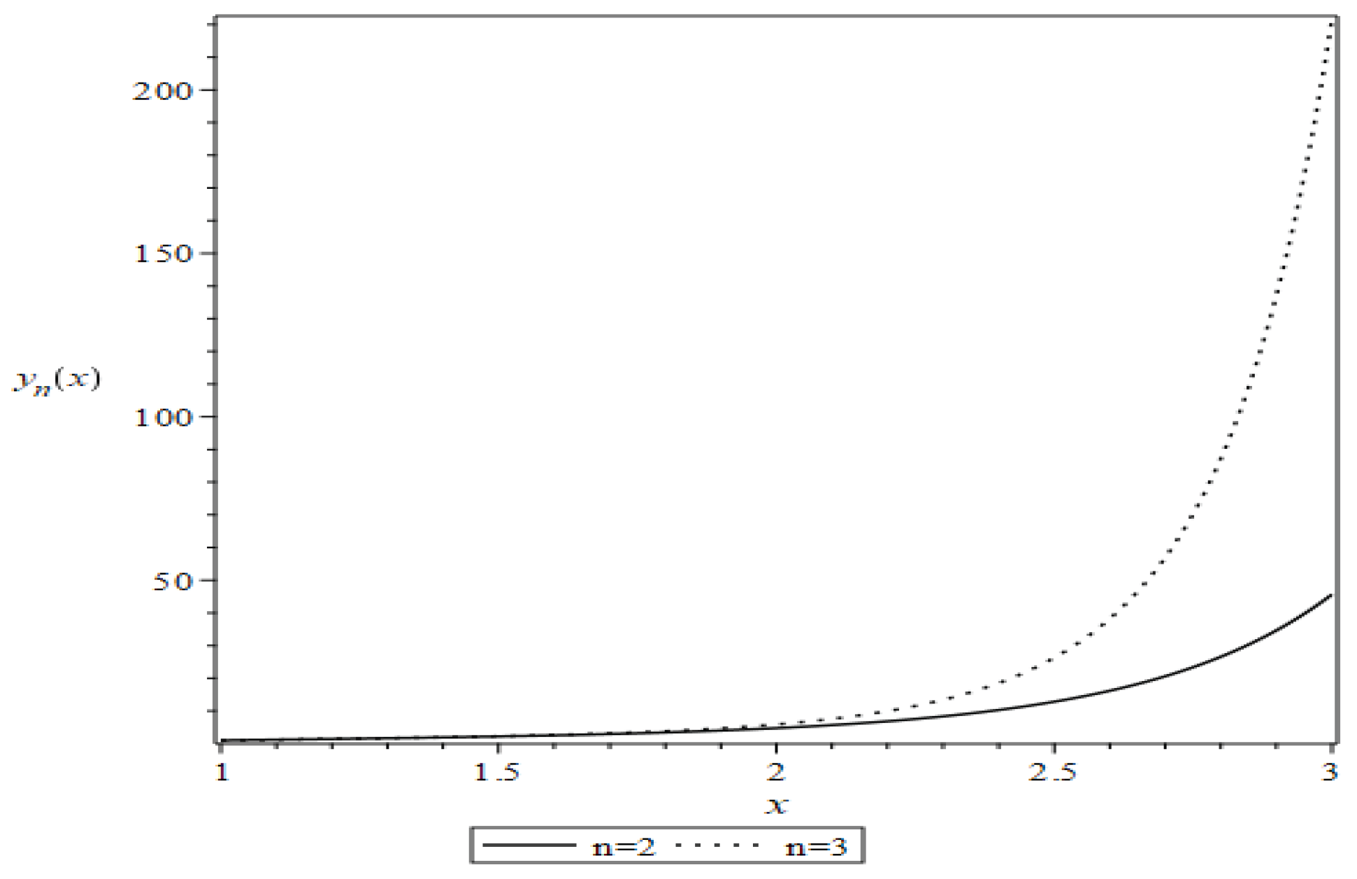

Table 1.
The Polynomials , and
| 0 | 0 | 1 | 0 |
| 1 | 1 | 0 | 0 |
| 2 | 0 | -1 | |
| 3 | 0 | ||
| 4 | |||
| 5 | |||
| 6 |
|
|
|
| 7 |
|
|
Table 2.
Degrees of the Polynomials , and
| Polynomial | Degree is even) |
Degree is odd) |
|---|---|---|
Table 3.
The Polynomials , and for .
| 0 | 0 | 1 | 0 |
| 1 | 1 | 0 | 0 |
| 2 | 0 | -1 | |
| 3 | 0 | ||
| 4 | |||
| 5 | |||
| 6 | |||
| 7 |
Disclaimer/Publisher’s Note: The statements, opinions and data contained in all publications are solely those of the individual author(s) and contributor(s) and not of MDPI and/or the editor(s). MDPI and/or the editor(s) disclaim responsibility for any injury to people or property resulting from any ideas, methods, instructions or products referred to in the content. |
© 2025 by the authors. Licensee MDPI, Basel, Switzerland. This article is an open access article distributed under the terms and conditions of the Creative Commons Attribution (CC BY) license (http://creativecommons.org/licenses/by/4.0/).
Copyright: This open access article is published under a Creative Commons CC BY 4.0 license, which permit the free download, distribution, and reuse, provided that the author and preprint are cited in any reuse.


