
Submitted:
18 May 2025
Posted:
19 May 2025
You are already at the latest version
Abstract
Cochin backwater region in Southern India is one of the most dynamic estuaries, strongly influenced by seasonal river runoff and seawater intrusion. This study explores the rela-tionship between monsoonal rains, salinity, and stable isotopic composition (δ¹⁸O and δ¹³C) to estimate the contribution of freshwater fluxes at different seasonal intervals for the Cochin Backwater (CBW) estuary. Seasonal variations in oxygen isotopes and salinity re-vealed distinct trends indicative of freshwater-seawater mixing dynamics. The compari-son of Local and Global Meteoric Water Lines highlighted enriched isotope values during the pre-monsoon season, showing significant evaporation effects. Carbon (C) isotopic analysis in dissolved inorganic matter (δ¹³CDIC) at 17 stations during the pre-monsoon season revealed spatially distinct carbon dynamics zones, influenced by various sources. These characteristic zones were Zone 1, dominated by seawater, exhibited heavier δ¹³CDIC values; Zone 2 showing significant contributions of lighter terrestrial δ¹³C; while Zone 3 reflected inputs from regional and local paddy fields with a distinct C3 isotopic signature (-25‰), modified by estuarine productivity. In addition, different advanced machine learning techniques were tested to improve analysis and prediction of seasonal variations in isotopic composition and salinity. The combination of these advanced machine learn-ing models not only improved the predictive accuracy of seasonal freshwater fluxes but also provided a robust framework for understanding the estuarine ecosystem and would pave way for better management and conservation strategies.
Keywords:
Seasonal Freshwater Flux
; Stable Isotopes
; Machine Learning
; Salinity
; Estuarine Dynamics
1. Introduction
Estuaries are dynamic systems adjacent to coastal regions that exhibit seasonal variability in productivity due to differential fluxes of freshwater from rivers. Globally, estuaries function as crucial interfaces between terrestrial and marine ecosystems, supporting high biodiversity and providing ecosystem services such as nutrient cycling, carbon sequestration, and fisheries support [1]. Monsoonal estuaries, a semi-enclosed coastal body of water that has a free or regulated connection with the open sea, is a unique feature in southern India. These monsoonal estuaries offer an environment for understanding freshwater fluxes due to the characteristic mixing pattern denoting differential seawater influx, and freshwater input from continental runoff. The seasonal hydrological variability observed in monsoonal estuaries of southern India mirrors patterns in other estuarine systems worldwide, such as the Mekong Delta in Southeast Asia and the Amazon Estuary in South America, where freshwater influx, tidal regimes, and anthropogenic pressures collectively shape estuarine dynamics [1,2]. Comparative studies across these diverse geographic regions can enhance our understanding of estuarine resilience and responses to climate change and human activities on a global scale [3]. In that context, the current study was conducted in one of the largest monsoonal estuaries in southern Indian i.e., Cochin Back Water (CBW) estuary [4,5]. Tides in these estuaries are semi-diurnal with an average tidal height of 1 m, and the impact of anthropogenic interventions on the estuarine system is rather high and its geochemical dynamics is well-studied [5,6,7,8].
Freshwater entry into the CBW estuary occurs primarily through six rivers, Periyar, Muvattupuzha, Pampa, Achankovil, Manimala, and Meenachil. During the dry season, the runoff from the upstream area is minimal, promoting saline water intrusion into the low-lying paddy fields of CBW [9]. Unlike perennial rivers, such as Hooghly, which drain into the Bay of Bengal, forming an estuary near Sunderban [10], Southern Indian rivers are devoid of any glacial meltwater input during dry seasons. The contribution of freshwater to the estuary can be estimated at seasonal time intervals by differential mixing of seawater and freshwater, and this process can be quantified using data on salinity and δ18O ratio in estuary water [11,12]. Stable isotopic approaches, particularly the use of δ18O, δD, and δ13C signatures, have proven to be robust tools in tracing water sources, salinity gradients, and biogeochemical dynamics across diverse estuarine systems worldwide, providing critical insights into the effects of climate variability, land use change, and anthropogenic pressure on estuarine carbon cycling [13,14]. While δ18O and δD ratios are useful in predicting the mixing and evaporation processes, δ13C in Dissolved Inorganic Carbon (DIC) enable an understanding of both mixing and productivity or carbon uptake by the biota in the estuarine system [10].
Analysis of stable isotope data coupled with advanced machine learning techniques will enhance the analysis and prediction of seasonal variations in isotopic composition and salinity [15,16]. AI techniques, such as Artificial Neural Networks (ANN), Adaptive Neuro-Fuzzy Inference Systems (ANFIS), Support Vector Machines (SVM), Radial Function Based Neural Network (RBNN), Random Forest (RF), K-Nearest Neighbour (KNN) have become increasingly popular for addressing complex problems across various research domains [15,16,17,18,19]. These techniques excel at modeling complex nonlinear systems, effectively compensating for the limitations of traditional numerical models. ANN, ANFIS, and SVM are advanced computational techniques increasingly applied in the study of stable isotopes in estuarine environments. These methods enhance the understanding of complex ecological interactions and isotopic compositions, providing valuable insights into environmental changes. ANNs are effective in modelling complex ecosystems, as demonstrated in studies predicting phytoplankton blooms in estuaries [18]. SVMs have been utilized alongside ANNs to estimate isotopic compositions, salinity, and temperature, showing competitive accuracy in predictions [15].
In a particular case study from the Mediterranean Sea, three predictive models were developed using ANN, RF and SVM involving five key variables: (i–ii) geographic coordinates (longitude and latitude), (iii) year, (iv) month, and (v) depth. Among these, RF model demonstrated the highest prediction accuracy during the querying phase, achieving a mean absolute percentage error (MAPE) of approximately 4.98% for isotope composition, below 0.20% for salinity, and around 2.44% for temperature. Despite the advantages of these computational techniques and their predication accuracy, traditional methods still play a crucial role in hydro-environmental research, particularly in validating and complementing findings from machine learning models [15]. Employing AI models for δD and δ¹⁸O estimation of freshwater seawater interplay in the estuarine system in the Asian context is very much lacking, and the current study would represent a novel and valuable contribution to the costal research literature in the Asian region. The objective of using machine learning algorithms in this study was to develop a simple, and accurate model for estimating δ¹⁸O and δ¹³C isotopes in the CBW estuary. This was achieved by employing advanced machine learning techniques, including Gradient Boosting Machines (GBM), Gaussian Process Regression (GPR), Classification and Regression Tree (CART), and Extreme Learning Machines (ELM) [20,21,22]. These models were chosen for their ability to capture non-linear relationships, handle high-dimensional data, and quantify uncertainties in predictions. The models were rigorously evaluated for their accuracy, efficiency, and potential to serve as reliable alternatives to traditional isotope analysis methods, offering a robust framework for understanding seasonal freshwater fluxes and estuarine dynamics of the India sub-continent.
In the current study, we explored the relationship between salinity, stable isotopic composition, and freshwater fluxes in the CBW estuary across different seasons. We used existing data from the Arabian Sea to establish seawater δ18O and salinity baselines [23,24] and adopted seasonal rainwater composition from previous studies [25]. By analyzing productivity patterns and their link to salinity and freshwater input (δ18O), we identified distinct zones within the estuary based on varying freshwater influence and productivity levels. To classify these estuarine zones, we combined salinity and isotope data with spatial and temporal patterns, and used applied machine learning techniques like GBM, GPR, CART and ELM, and conventional machine learning techniques like RF, KNN, SVM to model and predict changes in isotopic composition, and evaluate the performance metrics of the used techniques
2. Materials and Methods
2.1. Study Area
Based on its dimensions, CBW is the largest estuarine system along the west coast of India and belongs to the Vembanad-Kol wetland system, one of the three Ramsar sites in Kerala that extends from Munambam (10° 10ʹ 00ʺ N, 76°10ʹ 15ʺ E) in the north to Alappuzha (09° 30ʹ 00ʺ N, 76° 28ʹ 10ʺ E) in the south for 96.5 km in length (Figure 1). The width varies from 450 m to 4 km, and the depth ranges from 15 m at the Cochin Inlet to 3 m near the head, with an average depth of 1.5 meters. The barrier spits are interrupted by tidal inlets at two locations (i) Munambam inlet in the north and (ii) Cochin inlet in the middle.
The present study was conducted on CBW and Vembanad Lake, situated at the southern tip of the Indian subcontinent. This region experiences three distinct seasons: Pre-Monsoon (PM, April–May), Southwest Monsoon (SWM, June–September), and Northeast Monsoon (NEM, October–December). During the monsoon season, the influx of freshwater significantly increases due to heavy precipitation, while the non-monsoon season (January–March) is characterized by reduced riverine input and dominant tidal forcing, leading to higher salinity levels in the estuary [11,26]. Water samples for δ¹⁸O and salinity analysis were collected fortnightly during high and low tides for a 1-year period between October to September of subsequent year (Table 1). Additionally, a spatial survey covering 17 sites (Figure 1, Table 2) was conducted in the pre-monsoon period (March-May) to document variability in isotopic composition and salinity.
Figure 1.
Map of the Cochin backwater with sampling locations. Temporal sampling location is given in filled circles (samples in Table 1); whereas, hollow circles represent locations of spatial sampling (samples in Table 2).
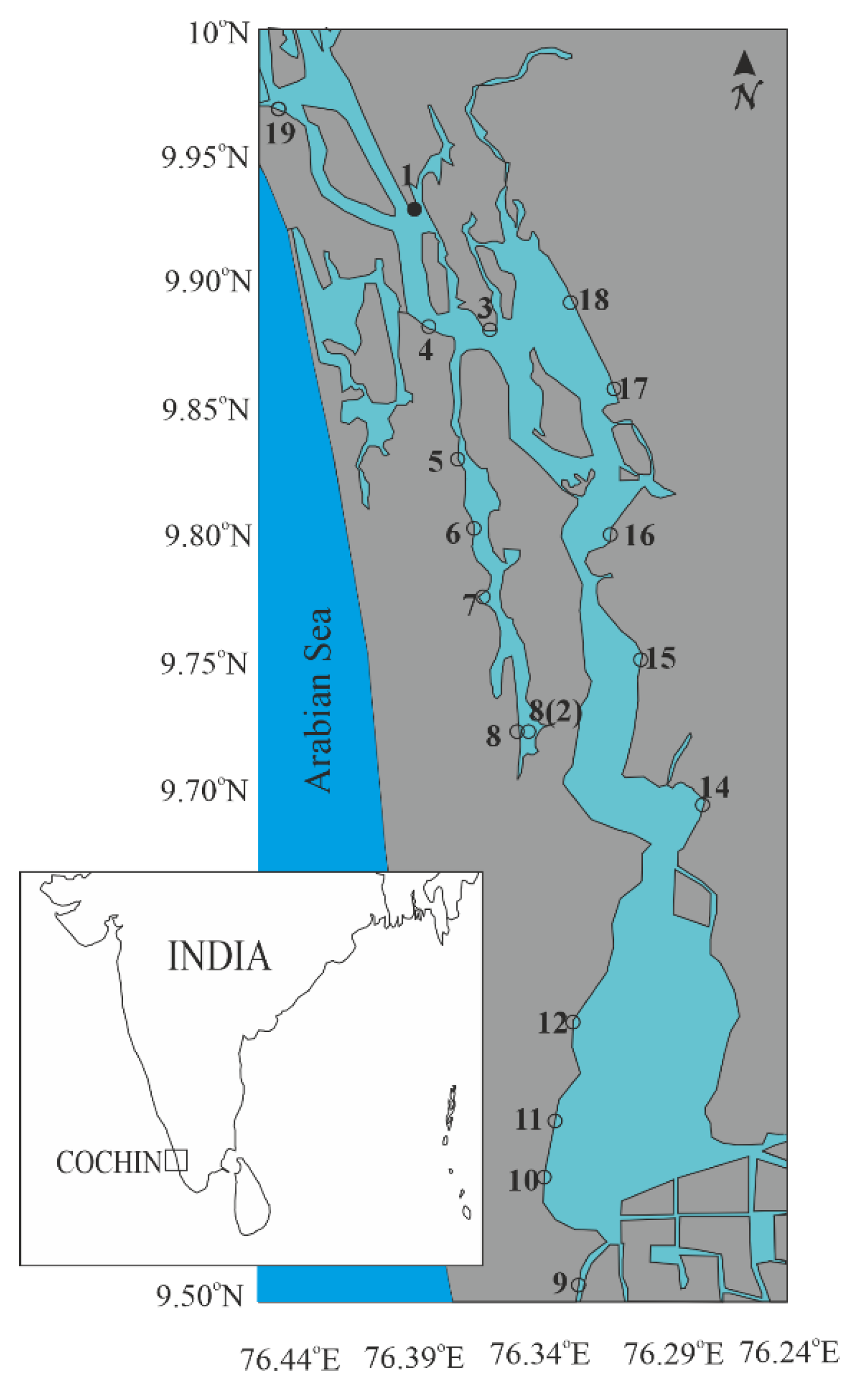

Table 1.
Measured salinity and oxygen isotopic composition of Cochin backwater collected biweekly during both low tide and high tides at sample site 1 as indicated in Figure 1.
Table 1.
Measured salinity and oxygen isotopic composition of Cochin backwater collected biweekly during both low tide and high tides at sample site 1 as indicated in Figure 1.
| Date of Sample Collection | Seasons | δ18OVSMOW (‰) | Salinity | ||
| High tide | Low tide | High tide | Low tide | ||
| 4-Oct | North-East Monsoon | -2.84 | 0.2 | ||
| 18-Oct | -1.87 | -1.9 | 8.5 | 5.1 | |
| 2-Nov | -1.19 | -3.49 | 12.6 | 11.1 | |
| 16-Nov | -4.69 | -4.21 | 1.9 | 1.3 | |
| 2-Dec | -2.44 | -3 | 11.5 | 7.1 | |
| 16-Dec | -1.15 | -2.22 | 19.4 | 12.3 | |
| 31-Dec | -1.15 | -1.54 | 20 | 16.2 | |
| 15-Jan | -0.96 | -1.86 | 19.6 | 17.8 | |
| 30-Jan | -1.23 | -0.7 | 21.1 | 18 | |
| 13-Feb | Pre-Monsoon | -0.41 | -0.74 | 21.7 | 17.1 |
| 28-Feb | -0.3 | -1.24 | 20.5 | 18.6 | |
| 15-Mar | -0.58 | -0.78 | 18.5 | 18.1 | |
| 15-Apr | -0.75 | -1.1 | 20.5 | 16.6 | |
| 14-May | -0.72 | -0.47 | 21.6 | 20.3 | |
| 27-May | -1.01 | -1.09 | 7.8 | 4.9 | |
| 14-Jun | South West Monsoon | -3.72 | -3.69 | 0.2 | 0.1 |
| 27-Jun | -3.2 | -3.29 | 0.2 | 0.2 | |
| 11-Jul | -2.83 | -2.68 | 1 | 2.6 | |
| 26-Jul | -2.66 | -2.58 | 2.5 | 0.5 | |
| 11-Aug | -2.26 | -2.2 | 2.8 | 4 | |
| 26-Aug | -2.74 | -2.58 | 0.7 | 0.7 | |
| 8-Sep | -2.01 | -2.42 | 10.2 | 2.9 | |
| 25-Sep | -5.01 | 0.1 | |||
Table 2.
Hydrological parameters of Cochin backwater collected during pre-monsoon season.
| Sl. No | Location | Lat (oN) | Long (oE) | Salinity (PSU) |
δ18O (‰ VSMOW) |
δ13CDIC (‰ VPDB) |
| 1 | Thevara ferry | 9.93 | 76.30 | 0.10 | 0.42 | -5.60 |
| 2 | Panangad | 9.88 | 76.33 | 18.80 | 0.54 | -5.64 |
| 3 | Arror | 9.88 | 76.31 | 17.60 | 0.89 | -10.52 |
| 4 | Kudapuram (Eramallor) | 9.83 | 76.32 | 15.70 | NA | -9.01 |
| 5 | Kodamthuruthu (Kuthiathodu) | 9.80 | 76.33 | 13.10 | 2.49 | -9.60 |
| 6 | Thykkatusherry | 9.77 | 76.33 | 11.70 | 3.31 | -11.10 |
| 7A | Vyalar | 9.72 | 76.43 | 10.40 | 1.52 | -9.62 |
| 7B | Vyalar | 9.72 | 76.43 | 10.40 | 0.43 | -8.58 |
| 8 | Punnamada | 9.51 | 76.35 | 2.10 | 0.50 | -14.09 |
| 9 | Aaryad | 9.54 | 76.35 | 0.10 | 1.76 | -17.23 |
| 10 | Pallathuserry | 9.56 | 76.36 | 0.10 | 0.53 | -21.34 |
| 11 | Muhamma | 9.60 | 76.36 | 3.40 | 1.23 | -17.03 |
| 12 | Thalayazham (Puthanpalam) | 9.69 | 76.41 | 10.40 | 2.00 | -11.97 |
| 13 | Vaikom | 9.75 | 76.39 | 11.60 | 3.06 | -9.33 |
| 14 | Kulasekaramagalam (Mekara) | 9.80 | 76.38 | 11.90 | 0.78 | -8.04 |
| 15 | Punnakkaveli (South Paravoor) | 9.86 | 76.38 | 12.45 | 2.45 | -7.74 |
| 16 | Chavakakadavuamera (Udayamperoor) | 9.89 | 76.36 | 16.40 | 1.59 | -7.20 |
| 17 | Fort Kochi | 9.97 | 76.24 | 28.00 | -1.75 | -2.90 |
2.2. Sample collection and Analysis
Water samples were collected in 50 ml HDPE bottles and stored until analysis. Measurements were conducted using the CO2-H2O equilibration method [27,28] on a Thermo Fisher MAT-253 isotope ratio mass spectrometer coupled with a GasBench II. Reproducibility values for δ¹⁸O were 0.08‰. Water samples were analyzed immediately after collection using a conductivity probe (Orion, range 0.1 to 42, accuracy ±0.1) connected to a Thermo Scientific Orion 5-star multi-meter. The conductivity probe was standardized with Orion conductivity standards (147 μS/cm, 1413 μS/cm, and 12.9 mS/cm). For δ¹³C-DIC, water samples were collected in glass amber bottles with butyl rubber septa, treated with 1 ml of saturated HgCl₂ solution to inhibit biological activity, and stored. δ¹³C-DIC was measured by acidifying 2 ml of water with 0.5 ml of 100% orthophosphoric acid [29]. Standards, including NBS19 and MARJ1, were analyzed for calibration with a standard deviation of 0.09‰ for δ¹³C [30]. Rainfall data were obtained from the nearest weather station on Willingdon Island (latitude 9° 57ʹ 14ʺ N, longitude 76° 16ʹ 06ʺ E) (http://www.tutiempo.net).
2.3. Machine Learning Methodology
Advanced machine learning techniques were employed to estimate and predict δ¹⁸O and δ¹³C isotopic compositions and salinity in the estuary as shown in the Figure 2. The models used include GBM for feature importance analysis and capturing non-linear relationships, GPR for uncertainty quantification and high prediction accuracy, ELM for efficient processing of high-dimensional data, RBNN for modeling non-linear patterns in isotopic and hydrological data, and CART for interpretable classification of estuarine zones. In addition, established conventional machine learning techniques like RF, KNN, SVM that have been sued in established isotopic predication studies were also used to model and predict changes in isotopic composition.
The data preprocessing included all continuous variables, including salinity and isotopic ratios. All the data were normalized to ensure compatibility across models. All the missing values were addressed using statistical imputation methods. Model Training and Evaluation step included dividing the data into training (60%), validation (20%), and test (20%) subsets. K-fold cross-validation was employed to ensure robust model evaluation. Determination of performance metrics included Root Mean Square Error (RMSE), Mean Absolute Percentage Error (MAPE), and Coefficient of Determination (R²). Feature Analysis and Interpretation was done using GBM, that provided feature importance rankings to identify key drivers of isotopic and salinity variations. GPR and CART enabled spatial and temporal classification of estuarine zones, revealing insights into monsoonal and non-monsoonal dynamics.
3. Results
3.1. Seasonal and Spatial Variations in δ¹⁸O and Salinity
The seasonal data revealed significant oscillations in δ¹⁸O and salinity values, irrespective of tidal phases as shown in Figure 3. During the North East Monsoon (NEM) period (October–December), δ¹⁸O values ranged from -4.69‰ to -1.15‰, with salinity values between 20 and 0.2. The Pre-Monsoon (April–May) period exhibited δ¹⁸O values from -1.1‰ to -0.47‰, with corresponding salinity values from 21.6 to 4.9. In the South West Monsoon (SWM), δ¹⁸O reached its lowest value of -5‰ during low tide and increased to -1‰ during high tide. The positive correlation between δ¹⁸O and salinity was evident across all seasons, though the slope of the best-fit line during the SWM was shallower than in other periods. Spatial variations were pronounced, with δ¹⁸O values ranging from -1.75‰ to 3.31‰ and salinity values spanning from 0.1 to 28.0 across different stations. Salinity and isotopic values varied significantly across the studied area and three distinct zones were evident. These were classified as Zone 1 (influenced by the Periyar River): salinity ranged from 0.1 to 28.0, δ¹⁸O varied between 0.7‰ and -0.6‰, and δ¹³C ranged from -2.9‰ to -10.5‰. Zone 2 (other freshwater sources): salinity ranged from 10.3 to 15.7, δ¹⁸O varied from 2.2‰ to -0.5‰, and δ¹³C ranged from -7.7‰ to -11.9‰. And Zone 3 (Vembanad Lake): Salinity ranged from 0.1 to 3.4, δ¹⁸O varied from 2.03‰ to -0.65‰, and δ¹³C ranged from -14.08‰ to -21.3‰.
3.2. Performance Metrics for Machine Learning Models
The performance metrics of all the used machine learning models are summarized in Table 3. For salinity prediction, the GBM model showed the highest accuracy, with the lowest RMSE (0.0993) and the highest R² (0.9563). For δ¹⁸O prediction, the KNN model performed best, achieving an RMSE of 0.1703, an R² of 0.5039, and a MAPE of 29.87%. The RF model also showed competitive performance (RMSE: 0.2101, R²: 0.2451), while the SVM model exhibited lower predictive power with reduced R² values. For δ¹³C prediction, models such as CART, ELM, and RBNN performed poorly, with negative R² values suggesting overfitting or insufficient training data. Low tide salinity was identified as the most significant predictor for high tide salinity in the GBM model. Geographic factors, including latitude and longitude, played a crucial role in δ¹⁸O and δ¹³C predictions. Models like GPR, CART, and RBNN also displayed negative R² values, indicating the necessity for further dataset expansion and model refinement.
4. Discussion
4.1. Seasonal and Spatial Variations in δ¹⁸O and Salinity
The salinity-δ18O relationship is a valuable tool for understanding the temporal mixing pattern of freshwater and seawater in estuaries around the world [31,32,33]. The surface-water salinity-oxygen isotopes of CBW showed two distinct trends defining the summer and winter composition. This large difference between salinity and water δ18O is due to the mixing of a variable amount of fresh water by the rivers draining the catchment and the saline Arabian Sea water. The rainwater δ18O during the monsoon season dominates the river water value, which varies between -1.0 ‰ and -3 ‰, while groundwater remains nearly invariant seasonally with a composition of -3.7 to -5.2 ‰ [34]. The seawater input into the estuary is isotopically heavier, with values between 1 and 0 ‰ in the Arabian Sea region. The difference between the salinity values measured during high and low tides was maximum during the summer season and minimum during the monsoon season. This implies that the extent of mixing of surface water is maximum in the monsoon season and minimum in the summer. The overall relationship between water δ18O and salinity is defined by δ18O = 0.1259 (salinity) -3.31, with a regression coefficient value of 0.7 (Figure 4).
4.2. δ18O Relationship with Salinity
Surface water salinity depends mainly on freshwater drainage, which carries a signature of rainwater during the wet period and groundwater during the dry period. The annual salinity varies from 21.7 to 0.1 (Table 1). The lowest surface salinity coincides with a period of SWM, where precipitation and catchment runoff reach their maximum. Maximum salinity was observed during the pre-monsoon period, wherein seawater intrusion was prominent. It was evident that the CBW region experienced diurnal and monthly tidal influences, which varied seasonally with the extent of seawater intrusion into the coastal area. As a function of these influences, the CBW estuary was classified into three zones based on its physiographical and hydrographical aspects. Zone 1, the region from the Cochin inlet to Perumpalam Island, is influenced by seawater from the Arabian Sea. Zone 2, From Perumpalam Island to Thanneermukkam Bund, is characterized by the mixing of freshwater from riverine input and seawater from the Arabian Sea. Zone 3 is dominated by freshwater. As seen in Figure 5, Zone 1 has a δ18O-Salinity relationship slope of 0.03 with a positive correlation with an R2 of 0.37. In comparison, Zone 2 had a steep slope of 0.5, with a positive correlation with an R2 of 0.6. Zone 3 had a negative slope of -0.9 with a weak R2 value of 0.05.
4.3. δ18O-δD Relationship of CBW Estuary
A total of 17 surface water samples collected during the pre-monsoon season were analyzed for δD and δ18O. The results are plotted in Figure 6 and compared with the Global Meteoric Water Line (GMWL) and the Local Meteoric Water Line (LMWL) from published literature [35]. In a previous study, the stable isotopes of Vembanad Lake water samples have been documented to range from -20.2 to +17.0 ‰ and -5.6 to +3.3 ‰ for δD and δ18O, respectively [11]. The most isotopically depleted values were observed during the monsoon season, which could be attributed to the amount effect. In contrast, an enrichment in isotopic values was observed during the pre-monsoon period due to salinity mixing or evaporation. In our study, we carried out spatial sampling only during the pre-monsoon season, and the δD vs. δ18O plot is characterized by enriched δ values similar to earlier observations as shown in Figure 6 [11]. The ingression of saline seawater with enriched isotope values also contributed to overall isotope observations in the estuary. The gradual decrease in the δ18O and δD values suggests that either excess evaporation or the enhanced contribution of seawater caused a compositional shift during the pre-monsoon season.
4.4. Freshwater Flux in Comparison with the Seasonal Rainfall
In an estuarine setting, the source of freshwater can vary and each of these freshwater sources have unique δ18O values, although the salinity of these sources is minimal. Previously reported δ18O values of the NEM from this region are -10‰ and -2‰ for the Premonsoon and -5‰ for the SWM [25,35]. These values are close (-1.8 to -5‰) to the river water composition measured at a seasonal interval in the region [34]. Using these δ18O values as freshwater end members, and measured average δ18O of estuarine waters, the relative contribution of freshwater can be ascertained using the below mass balance equation.
where sw, rw, and ew refer to seawater, rainwater, and estuarine water, respectively, and F indicates the flux parameter.
Fsw × δ18Osw + Frw × δ18Orw = δ18Oew
Fsw + Frw = 100
Percentage (%) = [δ18Oew − δ18Osw]/ [δ18Orw − δ18Osw]
The region receives rainfall distributed across three distinct rainfall seasons and is characterized by unique isotopic ratios [25,35,36]. The monthly mean and daily rainfall data of the study region was obtained from the Willingdon station, located ~3 km from the site of monthly observation. The indicated that in almost all years, rainfall is maximum from June to August coinciding with the SW monsoon (Figure 7 - Bottom panel). Based on the amount of rainfall and δ18O offset, the percentage contribution of freshwater was estimated and is shown in Figure 7 (Top panel). It was evident that freshwater flux into CBW estuary is primarily driven by runoff, which is major contributor during the monsoon season but drops significantly during the pre-monsoon and post-monsoon periods The water δ18O values of seasonal surface water was adapted from the tropical Chaliyar River basin to constrain the end-member composition. The catchment of this river is the Western Ghats in India, which receives the same rain source that feeds the rivers flowing into the Cochin estuary [34]. The surface water δ18O values for the river were -1.8 ‰, -1.2 ‰, and -4.5 ‰ for the NE monsoon, pre-monsoon, and monsoon seasons, respectively, while the freshwater percentages estimated were 25 %, 73 %, and 92 %, respectively. Furthermore, the estimates indicated that the fractional contribution (in %) of freshwater varies from 20-52 to% during the NE monsoon, 53-67 % during the pre-monsoon, and 50-100 % during the monsoon. High tide (HT) allows more seawater mixing in comparison to low tides.
4.5. Carbon Dynamics Using Salinity and δ13CDIC
Freshwater input to the estuary affects the net carbon isotopic composition of dissolved inorganic carbon, which is either derived from the degradation of organic matter present in the regional soil ecosystem or further modified due to water column productivity. Thus, δ13CDIC acts as a proxy for productivity in estuarine systems. However, the inorganic carbon reservoir in estuary water varies throughout the season, recording the flux of carbon due to silicate weathering [36]. The δ13CDIC observed during the present study (-2.9 ‰ to -21.34 ‰), with an average of -10.36 ‰, is comparable to a previous study in the region [12,37]. Figure 8 shows the conservative mixing curve of δ13CDIC, along with their respective actual values and salinity in three different zones of the Cochin Estuary. Among the five stations sampled in Zone 1, four stations were generally closer to the conservative mixing line, indicating the role of mixing of freshwater and seawater end members. The samples from Zone 2 were characterized by lower δ13CDIC values relative to the respective conservative mixing curve values. As observed in previous studies [12,37], the possible reason for the low δ13CDIC at these stations might be the dominant contribution from terrestrial inorganic carbon from the degradation of organics. The samples from Zone 3 are characterized by a lower δ13CDIC relative to the respective conservative mixing curves. This indicates that the carbon dynamics in Zone 3 are dictated by the runoff from the nearby paddy fields with a lighter C3 signature (-25 ‰), which is further modified owing to the productivity of the estuary [38].
4.6. Evaluating Machine Learning Models for Salinity and Isotopic Predictions
The study compared multiple machines learning models, including GBM, KNN, RF, SVM, CART, ELM, and RBNN, to predict salinity and isotopic ratios. The study’s comparison of various machine learning models highlights the challenges and opportunities in predicting salinity and isotopic compositions [15,16]. The GBM model emerged as the most reliable for salinity prediction, demonstrating the highest accuracy and predictive strength (Table 3). The strong performance of GBM can be attributed to its ability to capture complex, non-linear relationships between predictor variables, including tidal influence, temperature, and spatial factors. For δ¹⁸O prediction, the KNN model outperformed others, although overall performance metrics indicated room for improvement. The low performance of models like SVM for δ¹⁸O prediction suggests that certain machine learning approaches may not be well-suited for isotopic modeling without extensive parameter tuning and preprocessing (Table 3).
δ¹³C prediction faced significant challenges, with models like CART, ELM, and RBNN yielding negative R² values, suggesting overfitting or insufficient training data (Table 3). The poor performance of certain models highlights the need for expanded dataset and improved feature selection to enhance predictive accuracy. Given the complexity of δ¹³C variations, which are influenced by multiple environmental and biological factors, the integration of additional explanatory variables, such as dissolved organic carbon sources could enhance prediction accuracy. Additionally, the strong correlation between δ¹⁸O and salinity reinforces the utility of isotopes in tracing hydrochemical processes. Geographic parameters could also play a crucial role in model performance, indicating spatial influences on isotopic variations. The findings emphasize that while machine learning can be a powerful tool for hydrochemical predictions, robust data collection and model refinement are essential to improve generalizability and reliability across different environmental conditions.
5. Conclusions
The current study analyzed the seasonal variations in freshwater flux and isotopic compositions in the Cochin Backwater Estuary (CBW). It sheds light on the intricate interactions between monsoonal rains, salinity, and the use of stable isotopic markers and machine learning models. Seasonal monitoring revealed that the monsoon season contributes significantly (~77%) to the freshwater flux due to intense rainfall and riverine input, making the estuary predominantly freshwater during this period. The seasonal isotopic fingerprints revealed significant geographical and temporal patterns of intermixing at high and low tides. Detailed studies of δ¹³C in dissolved inorganic carbon (DIC) at 17 locations throughout the pre-monsoon season indicated regional diversity and zonation in biogeochemical processes. Zone 1 is predominantly impacted by saltwater enriched in δ¹³CDIC, whereas Zone 2 reflects terrestrial input from local sources. Zone 3 revealed the input of terrestrial runoff, mainly from rice fields, with lighter C3 plant signatures, which were further influenced by estuarine productivity. Comparison of the Local Meteoric Water Line to the Global Meteoric Water Line revealed the impacts of salinity mixing and evaporation, particularly during the pre-monsoon season, providing important insights into estuarine hydrology. In addition, we used machine learning models to improve our understanding of the predictive relationships between δ¹⁸O, salinity, and seasonal freshwater fluxes. The used models accurately captured the nonlinear dynamics of estuarine systems, providing powerful tools for analyzing the effects of seasonal variability and salinity mixing (GBM, KNN) on estuarine ecosystems. The study’s comparison of various machine learning models highlights that although machine learning could be a powerful tool for hydrochemical predictions, robust data collection and model refinement are crucial for improving reliability. In conclusion, the findings highlight the CBW’s distinctive function as an ecological hotspot in southern India, where monsoon and terrestrial inputs influence biogeochemical and production dynamics. The current study not only enhances our understanding of estuarine processes in the CBW but also provides a framework for employing advanced analytical and machine learning approaches in coastal ecosystem research.
Author Contributions
Conceptualization, P.K., P.G. and R.R.; methodology, H.R., P.K., F.T.; writing—original draft preparation, P.K., R.R., P.G. and H.R.; writing—review and editing, R.R. and P.K. All authors have read and agreed to the published version of the manuscript.
Funding
This research received no external funding.
Data Availability Statement
The data presented in this study are available on request from the corresponding author.
Acknowledgments
The authors are thankful to all the help obtained during the sampling and analysis throughout the project from the project members. RR is thankful to the research support provided through the grant CCEC01-1108-230167 from Qatar Research Development and Innovation Council.
Conflicts of Interest
The authors declare no conflicts of interest.
Abbreviations
The following abbreviations are used in this manuscript:
| CBW | Cochin Back Water |
| DIC | Dissolved Inorganic Carbon |
| PM | Pre-Monsoon |
| SWM | South West Monsoon |
| NEM | Northeast Monsoon |
| HT | High Tide |
| LT | Low Tide |
| NBS19 | National Bureau of Standards -19 |
| HDPE | High Density Polyethylene |
| ANN | Artificial Neural Networks |
| ANFIS | Adaptive Neuro-Fuzzy Inference Systems |
| SVM | Support Vector Machines |
| RBNN | Radial Function Based Neural Network |
| RF | Random Forest |
| KNN | K-Nearest Neighbor |
| GBM | Gradient Boosting Machines |
| GPR | Gaussian Process regression |
| CART | Classification and Regression Tree |
| ELM | Extreme Learning Machines |
| RMSE | Root Mean Square Error |
| MAPE | Mean Absolute Percentage Error |
References
- Day Jr, J.W., Kemp, W.M., Yáñez-Arancibia, A. and Crump, B.C. eds., 2012. Estuarine ecology. John Wiley & Sons.
- Dittmar, T. and Lara, R.J., 2001. Driving forces behind nutrient and organic matter dynamics in a mangrove tidal creek in North Brazil. Estuarine, Coastal and Shelf Science, 52(2), pp.249-259. [CrossRef]
- Cloern, J.E. and Jassby, A.D., 2010. Patterns and scales of phytoplankton variability in estuarine–coastal ecosystems. Estuaries and coasts, 33, pp.230-241. [CrossRef]
- Vijith V, Sundar D, Shetye SR (2009) Time-dependence of salinity in monsoonal estuaries. Estuar Coast Shelf Sci 85:601–608. [CrossRef]
- Qasim S, Gopinathan C (1969) Tidal cycle and the environmental features of Cochin Backwater (a tropical estuary). Proc Indian Acad Sci - Sect A Part 3, Math Sci 69:336–348. [CrossRef]
- Haldar, R., Khosa, R., Gosain, A.K. (2019). Impact of Anthropogenic Interventions on the Vembanad Lake System. In: Rathinasamy, M., Chandramouli, S., Phanindra, K., Mahesh, U. (eds) Water Resources and Environmental Engineering I. Springer, Singapore. [CrossRef]
- Kulk, G., George, G., Abdulaziz, A., Menon, N., Theenathayalan, V., Jayaram, C., Brewin, R. J., & Sathyendranath, S. (2020). Effect of Reduced Anthropogenic Activities on Water Quality in Lake Vembanad, India. Remote Sensing, 13(9), 1631. [CrossRef]
- Pranav, P., Roy, R., Jayaram, C., D’Costa, P. M., Choudhury, S. B., Menon, N. N., Nagamani, P., Sathyendranath, S., Abdulaziz, A., Sai, M. S., Sajhunneesa, T., & George, G. (2021). Seasonality in carbon chemistry of Cochin backwaters. Regional Studies in Marine Science, 46, 101893. [CrossRef]
- Shivaprasad A, Vinita J, Revichandran C, et al. (2013) Seasonal stratification and property distributions in a tropical estuary (Cochin estuary, west coast, India).
- Ghosh P, Chakrabarti R, Bhattacharya SK (2013) Short- and long-term temporal variations in salinity and the oxygen, carbon and hydrogen isotopic compositions of the Hooghly Estuary water, India. Chem Geol 335:118–127. [CrossRef]
- Nasir UP, Harikumar PS (2012) Hydrochemical and isotopic investigation of a tropical wetland system in the Indian sub-continent. Environ Earth Sci 66:111–119.
- Bhavya PS, Kumar S, Gupta GVM, et al. (2016) Carbon isotopic composition of suspended particulate matter and dissolved inorganic carbon in the Cochin estuary during post-monsoon. Curr Sci 110:.
- Raymond, P.A., Bauer, J.E., Caraco, N.F., Cole, J.J., Longworth, B. and Petsch, S.T., 2004. Controls on the variability of organic matter and dissolved inorganic carbon ages in northeast US rivers. Marine chemistry, 92(1-4), pp.353-366. [CrossRef]
- Bouillon, S., Borges, A.V., Castañeda-Moya, E., Diele, K., Dittmar, T., Duke, N.C., Kristensen, E., Lee, S.Y., Marchand, C., Middelburg, J.J. and Rivera-Monroy, V.H., 2008. Mangrove production and carbon sinks: a revision of global budget estimates. Global biogeochemical cycles, 22(2). [CrossRef]
- Astray, G., Soto, B., Barreiro, E., Gálvez, J. F., & Mejuto, J. C. (2021). Machine learning applied to the oxygen-18 isotopic composition, salinity and temperature/potential temperature in the mediterranean sea. Mathematics. [CrossRef]
- Cemek, B., Arslan, H., Küçüktopcu, E., & Simsek, H. (2022). Comparative analysis of machine learning techniques for estimating groundwater deuterium and oxygen-18 isotopes. Stochastic Environmental Research and Risk Assessment. [CrossRef]
- Noori, N., Kalin, L., & Isik, S. (2020). Water quality prediction using SWAT-ANN coupled approach. Journal of Hydrology. [CrossRef]
- Ly, Q. V., Nguyen, X. C., Lê, N. C., Truong, T. D., Hoang, T. H. T., Park, T. J., ... & Hur, J. (2021). Application of Machine Learning for eutrophication analysis and algal bloom prediction in an urban river: A 10-year study of the Han River, South Korea. Science of The Total Environment, 797, 149040. [CrossRef]
- Samalavičius, V., Gadeikienė, S., Žaržojus, G., Gadeikis, S., & Lekstutytė, I. (2024). Oxygen-18 prediction using machine learning in the Baltic Artesian Basin groundwater. Stochastic Environmental Research and Risk Assessment, 1-23. [CrossRef]
- Albuquerque, L. G., de Oliveira Roque, F., Valente-Neto, F., Koroiva, R., Buss, D. F., Baptista, D. F., Hepp, L. U., Kuhlmann, M. L., Sundar, S., Covich, A. P., & Pinto, J. O. P. (2021). Large-scale prediction of tropical stream water quality using Rough Sets Theory. Ecological Informatics. [CrossRef]
- Al Sudani, Z. A., & Salem, G. S. A. (2022). Evaporation rate prediction using advanced machine learning models: a comparative study. Advances in Meteorology, 2022(1), 1433835. [CrossRef]
- Dagher, D. H. (2024). Assessment of Using Machine and Deep Learning Applications in Surface Water Quantity and Quality Predictions: A Review. Journal of Water Resources and Geosciences, 3(2), 18-48.
- Singh A, Jani RA, Ramesh R (2010) Spatiotemporal variations of the δ18O-salinity relation in the northern Indian Ocean. Deep Sea Res Part I Oceanogr Res Pap 57:1422–1431. [CrossRef]
- Deshpande RD, Muraleedharan PM, Singh RL, et al. (2013) Spatio-temporal distributions of δ18O, δD and salinity in the Arabian Sea: Identifying processes and controls. Mar Chem 157:144–161.
- Lekshmy, P.R., Midhun, M., Ramesh, R. and Jani, R.A., 2014. 18O depletion in monsoon rain relates to large scale organized convection rather than the amount of rainfall. Scientific reports, 4, p.5661. [CrossRef]
- Rasheed K, Joseph KA, Balchand AN (1995) Impacts of harbour dredging on the coastal shoreline features around Cochin. In: Proceedings of the international conference on ‘Coastal Change. pp 943–948.
- Epstein S, Mayeda T (1953) Variation of O18 content of waters from natural sources. Geochim Cosmochim Acta 4:213–224. [CrossRef]
- Rangarajan R, Ghosh P (2011) Role of water contamination within the GC column of a GasBench II peripheral on the re-producibility of 18O/16O ratios in water samples. Isotopes Environ Health Stud 47:498–511. [CrossRef]
- Assayag N, Rivé K, Ader M, et al. (2006) Improved method for isotopic and quantitative analysis of dissolved inorganic carbon in natural water samples. Rapid Commun Mass Spectrom 20:2243–2251. [CrossRef]
- Rangarajan, R., Pathak, P., Banerjee, S. and Ghosh, P. (2021). Floating boat method for carbonate stable isotopic ratio determination in a GasBench II peripheral. Rapid Communications in Mass Spectrometry, 35(15), p.e9115. [CrossRef]
- Torgersen T (1979) Isotopic composition of river runoff on the US East Coast: Evaluation of stable isotope versus salinity plots for coastal water mass identification. J Geophys Res Ocean 84:3773–3775. [CrossRef]
- Fairbanks RG, Sverdlove M, Free R, et al. (1982) Vertical distribution and isotopic fractionation of living planktonic forami-nifera from the Panama Basin. Nature 298:841.
- Khim B-K, Park B-K, Yoon H Il (1997) Oxygen isotopic compositions of seawater in the Maxwell Bay of King George Island, west Antarctica. Geosci J 1:115.
- Hameed AS, Resmi TR, Suraj S, et al. (2015) Isotopic characterization and mass balance reveals groundwater recharge pattern in Chaliyar river basin, Kerala, India. J Hydrol Reg Stud 4:48–58. [CrossRef]
- Rahul, P. and Ghosh, P., 2019. Long term observations on stable isotope ratios in rainwater samples from twin stations over Southern India; identifying the role of amount effect, moisture source and rainout during the dual monsoons. Climate Dynamics, 52(11). [CrossRef]
- Warrier, C.U., Babu, M.P., Manjula, P., Velayudhan, K.T., Hameed, A.S. and Vasu, K., 2010. Isotopic characterization of dual monsoon precipitation–evidence from Kerala, India. Current Science, pp.1487-1495.
- Samanta S, Dalai TK, Tiwari SK, Rai SK (2018) Quantification of source contributions to the water budgets of the Ganga (Hooghly) River estuary, India. Mar Chem 207:42–54. [CrossRef]
- Bhavya PS, Kumar S, Gupta GVM, et al. (2018) Spatio-temporal variation in δ13CDIC of a tropical eutrophic estuary (Cochin estuary, India) and adjacent Arabian Sea. Cont Shelf Res 153:75–85. [CrossRef]
- Kaushal R, Ghosh P, Geilmann H (2016) Fingerprinting environmental conditions and related stress using stable isotopic composition of rice (Oryza sativa L.) grain organic matter. Ecol Indic 61:941–951. [CrossRef]
Figure 2.
Work flow of advanced machine learning techniques that were employed to estimate and predict δ¹⁸O and δ¹³C isotopic compositions and salinity in the estuary.
Figure 2.
Work flow of advanced machine learning techniques that were employed to estimate and predict δ¹⁸O and δ¹³C isotopic compositions and salinity in the estuary.
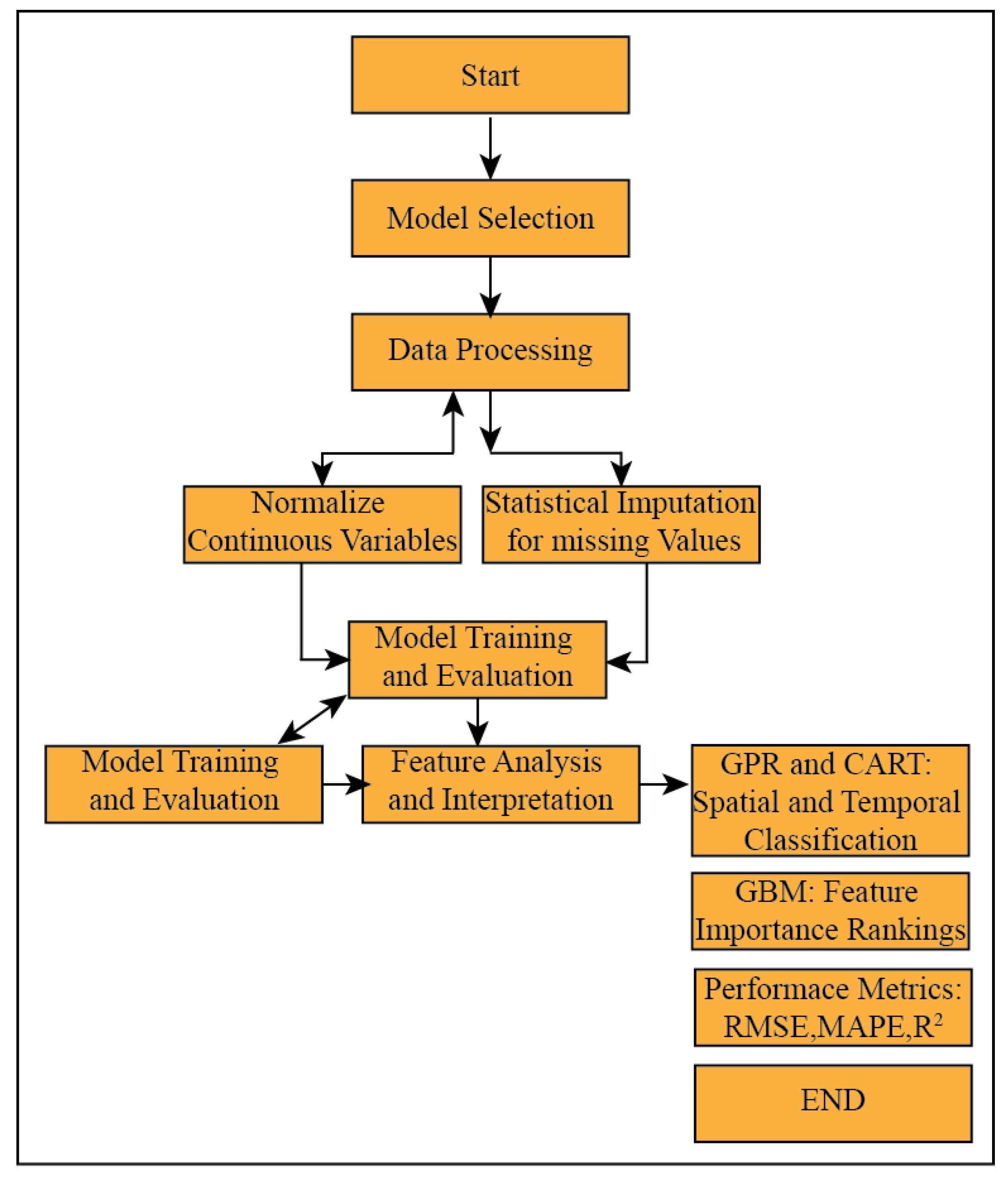
Figure 3.
The top panel shows high tide and low tide water δ18O measured, while the bottom panel shows salinity data measured in the collected water samples.
Figure 3.
The top panel shows high tide and low tide water δ18O measured, while the bottom panel shows salinity data measured in the collected water samples.
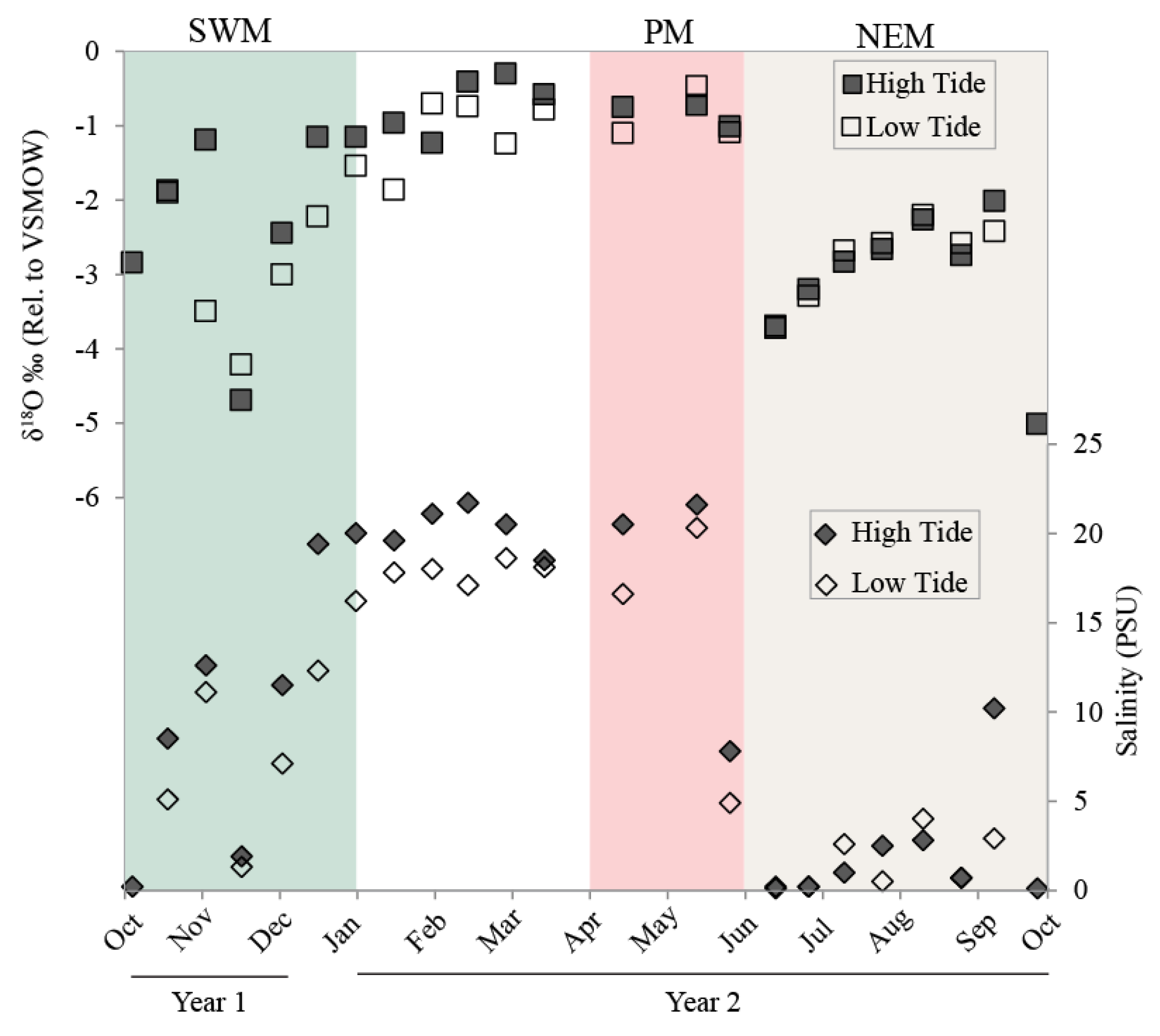
Figure 4.
Correlation plot between δ18O and salinity in the collected CBW samples indicating the mixing between freshwater and saline water.
Figure 4.
Correlation plot between δ18O and salinity in the collected CBW samples indicating the mixing between freshwater and saline water.
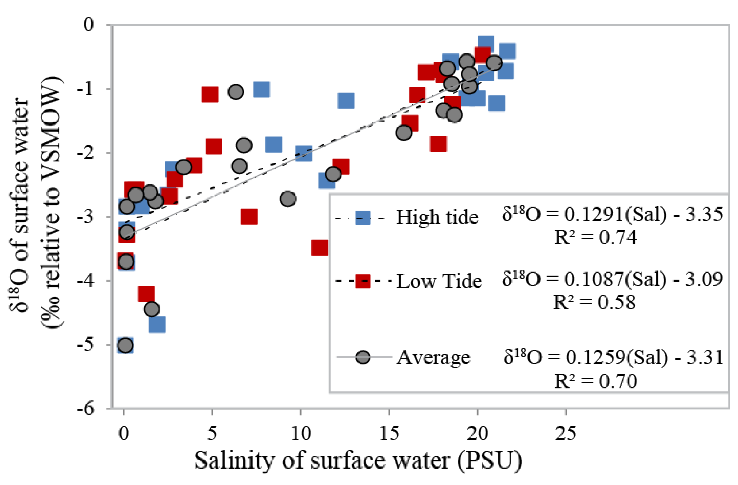
Figure 5.
δ18O-Salinity relationship indicating three different zones for collected pre-monsoon sample is shown.
Figure 5.
δ18O-Salinity relationship indicating three different zones for collected pre-monsoon sample is shown.
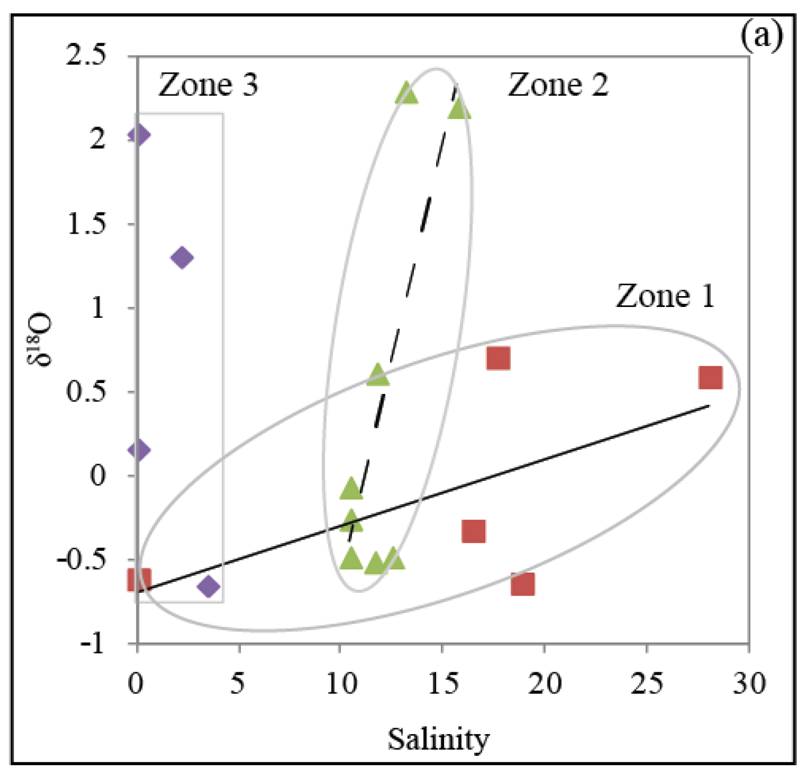
Figure 6.
Comparison of δ18O-δD regression line based on 18 surface water samples (Table 1) collected and compared with GMWL and LMWL.
Figure 6.
Comparison of δ18O-δD regression line based on 18 surface water samples (Table 1) collected and compared with GMWL and LMWL.
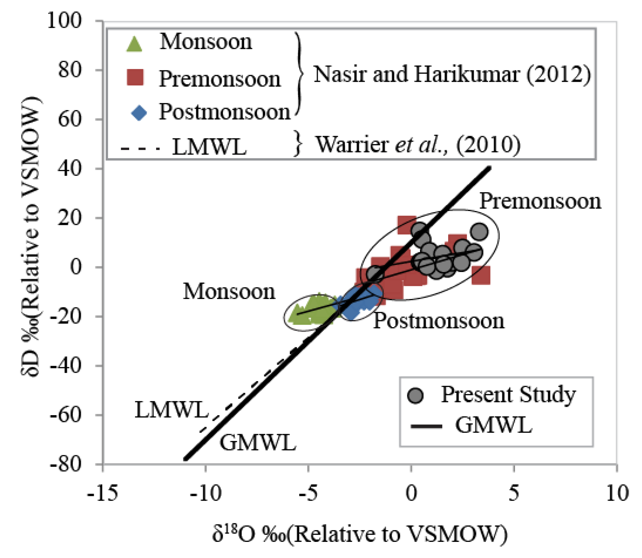
Figure 7.
Relative contribution of freshwater to the Cochin backwater at different times of the year calculated using δ18O of the freshwater end-member (Seasonal rainwater δ18O) and seawater.
Figure 7.
Relative contribution of freshwater to the Cochin backwater at different times of the year calculated using δ18O of the freshwater end-member (Seasonal rainwater δ18O) and seawater.
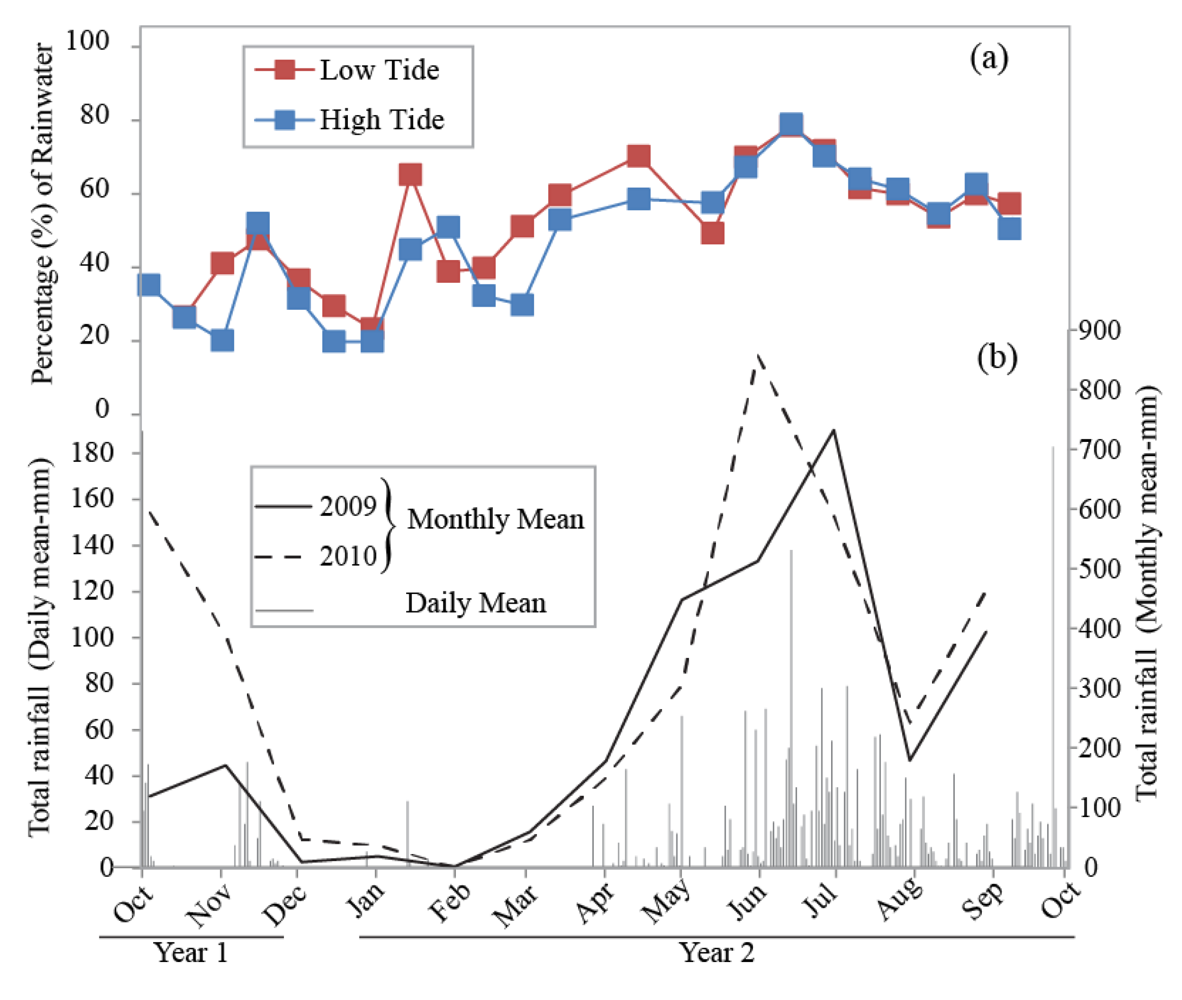
Figure 8.
δ13C-Salinity relationship along with the conservative mixing curve for CBW estuary.
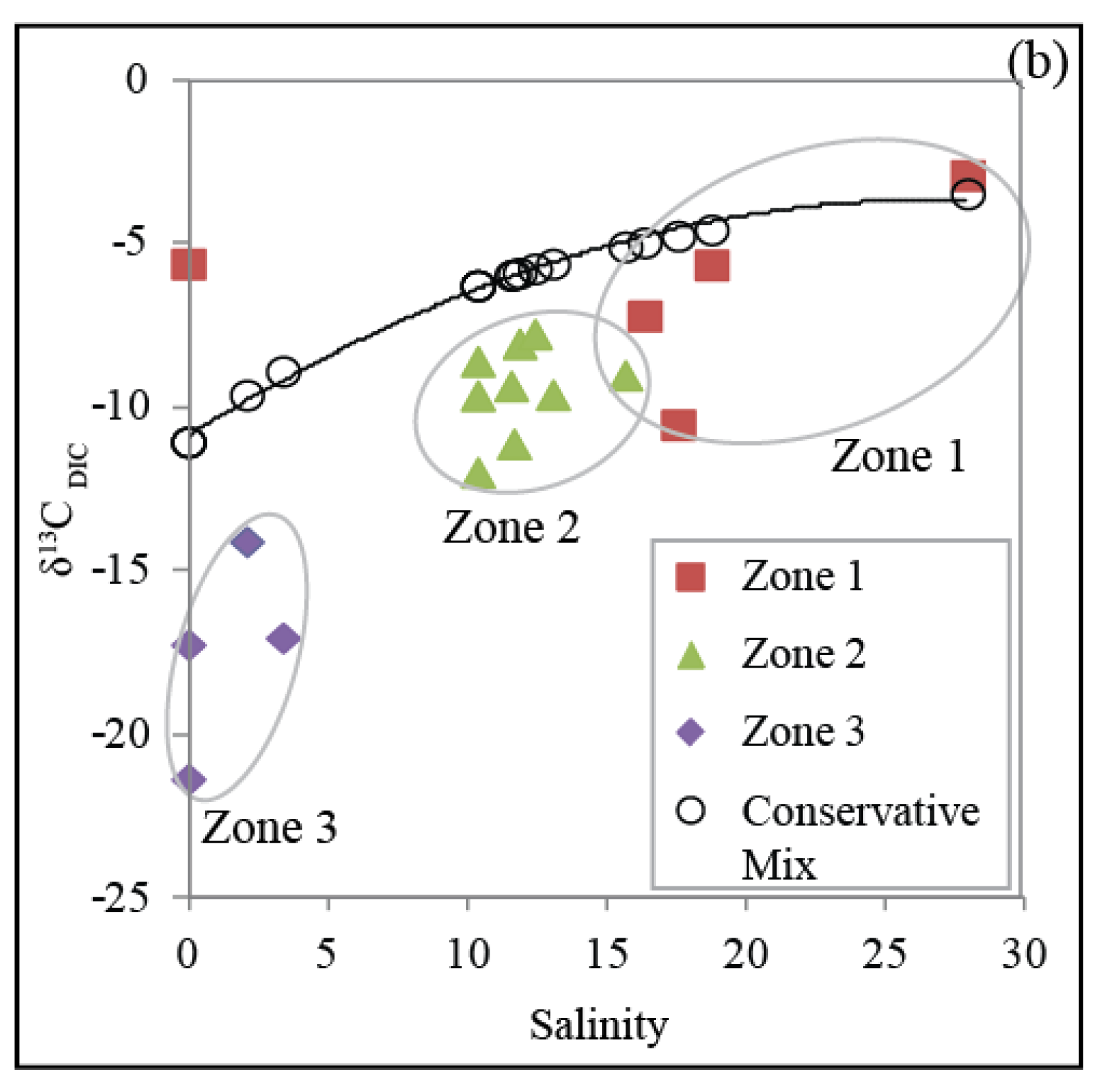
Table 3.
Performance Metrics of all machine learning models used in the study and the target parameter modelled.
Table 3.
Performance Metrics of all machine learning models used in the study and the target parameter modelled.
| Model | Target | RMSE | R² | MAPE (%) | T-Test (p-value) |
| GBM | Salinity | 0.0993 | 0.9563 | N/A | <0.001 |
| GPR | δ¹⁸O | 0.6298 | -5.7860 | N/A | 0.045 |
| CART | δ¹³C | 0.3449 | -2.0460 | N/A | 0.089 |
| ELM | δ¹⁸O | 0.9187 | -13.440 | N/A | 0.103 |
| ELM | δ¹³C | 0.7626 | -13.890 | N/A | 0.097 |
| RBNN | δ¹⁸O | 0.2869 | -0.4080 | N/A | <0.001 |
| RBNN | δ¹³C | 0.2626 | -0.7660 | N/A | <0.001 |
| RF | δ¹⁸O | 0.2101 | 0.2451 | 36.19 | <0.001 |
| RF | δ¹³C | 0.2489 | -0.5869 | 34.90 | 0.032 |
| SVM | δ¹⁸O | 0.2500 | -0.0695 | 39.16 | 0.071 |
| SVM | δ¹³C | 0.2556 | -0.6722 | 25.88 | 0.089 |
| KNN | δ¹⁸O | 0.1703 | 0.5039 | 29.87 | <0.001 |
Disclaimer/Publisher’s Note: The statements, opinions and data contained in all publications are solely those of the individual author(s) and contributor(s) and not of MDPI and/or the editor(s). MDPI and/or the editor(s) disclaim responsibility for any injury to people or property resulting from any ideas, methods, instructions or products referred to in the content. |
© 2025 by the authors. Licensee MDPI, Basel, Switzerland. This article is an open access article distributed under the terms and conditions of the Creative Commons Attribution (CC BY) license (http://creativecommons.org/licenses/by/4.0/).
Copyright: This open access article is published under a Creative Commons CC BY 4.0 license, which permit the free download, distribution, and reuse, provided that the author and preprint are cited in any reuse.


