
Submitted:
16 May 2025
Posted:
19 May 2025
You are already at the latest version
Abstract
To offer a viewpoint on convexity and connectedness inside intuitionistic fuzzy graphs (IFGs), the paper is devoted to the study of intuitionistic fuzzy geodetic convexity. The paper introduces an algorithm for precise identification and characterization of geodetic pathways in IFGs, supported by a Python program. Various properties of IF-geodetic convex sets such as IF-internal and IF-boundary vertices are obtained. Furthermore, this work introduces and characterizes the concepts of geodetic IF-cover, geodetic IF-basis, and geodetic IF-number. Additionally, the study develops the IF-geodetic Wiener index. The scope of the work explores the application of IF-geodetic cover in wireless mesh networks, focusing on the identification of gateway nodes. A practical implementation of the IF-geodetic Wiener index method in global human trading analysis underscores the real-world implications of the developed concepts.
Keywords:
intuitionistic fuzzy graph
; IF-geodetic convex
; geodetic IF-number
; geodetic IF-basis
; IF-internal vertices
; IF-boundary vertices
; IF-geodetic Wiener index
1. Introduction
The concept of fuzzy sets was introduced by Lotfi A. Zadeh [21] in 1965 and addresses ambiguity and imprecision in set theory. Zadeh researched fuzzy relations and how they work. Zadeh’s objective was to develop a theory that might regulate the imprecision and vagueness of a certain category in human thought, particularly in the areas of abstraction, information technology, and communication. In his study, Zadeh challenged a basic concept of probability theory. Each element in the universal set is assigned a value of 1 or 0 by the characteristic function in the crisp set. A generalized version of the characteristic function defined in a crisp set can be thought of as fuzzy set theory. Here, the items in the universal set are assigned within a predetermined range, indicating their membership grade. Subsequently, this function is referred to as a membership function, and the set that is produced is known as a fuzzy set. The membership function has a range of values from 0 to 1. Stated otherwise, the membership function’s values vary within the unit interval [0, 1].
Rosenfeld [1] is credited with organizing and developing the concept of fuzzy graphs. Yeh and Bang independently established fuzzy graph design in the meantime. Rosenfeld deduced the fuzzy equivalents of multiple concepts in graph theory. There is an extensive range of practical applications for fuzzy graphs. Numerous domains, including cluster analysis, group structure, pattern categorization, networking, management, and others, demonstrate their broad range of applications. Fuzzy graphs are more useful in real-world scenarios due to their extensive range of useful applications. Numerous other authors like P.S. Nair [5], Sunil Mathew and J.N. Mordeson [7,17], Sunitha and Vijayakumar [18] and R. Rajeshkumar and A. M. Anto [15] carried out many other groundbreaking studies in this area.
Atanassov [2] introduced a number of concepts related to intuitionistic fuzzy graphs (IFGs). The field of intuitionistic fuzzy sets and its applications has grown exponentially worldwide. This idea now encompasses the fields of information technology as well as traditional mathematics. The concept and associated features of intuitionistic fuzzy graphs were introduced by Parvathy and Karunambigai [14]. Additionally, Nagoor Gani covered a few more features of intuitionistic fuzzy graphs in [12]. In [8], Akram et al. offered various concepts and provided a precise definition of IFGs. Anto A.M. and Rajeshkumar R. [15] introduced the idea of IFGs having independent dominances.
This article starts with a brief description of the fundamentals of intuitionistic fuzzy graphs discussed in [10,15,20]. Later, based on a metric established in intuitionistic fuzzy graphs in [19], this study introduces novel ideas and approaches that make a substantial addition to the subject of intuitionistic fuzzy graph theory. We present the concept of intuitionistic fuzzy geodetic convexity, which offers an insightful view of convexity and connectedness in the context of intuitionistic fuzzy graphs (IFGs). A specially designed Python program for precisely finding and characterizing geodetic pathways in IFGs is presented along with a specialized algorithm for geodetic path identification in the study. The investigation also includes IF-internal and IF-boundary vertices in IF-geodetic convex sets. An important development in the field of IFGs is the creation of the Geodetic IF-Basis and Geodetic IF-number, providing tools for a thorough understanding and characterization of geodetic convexity. A novel concept, the Intuitionistic Fuzzy Geodetic Wiener Index (), is introduced, leveraging the framework of IF-geodesics. Furthermore, the application of IF-Geodetic Cover in a wireless mesh network is explored for the identification of gateway nodes, demonstrating its effectiveness in enhancing network connectivity and optimizing node placement for improved efficiency. In a practical application, the method is employed in global human trading analysis.
2. Preliminaries
We use the notion of Intuitionistic Fuzzy Graphs (IFGs) introduced by Karunambigai and Parvathi [14]. In this section, let us have a quick review of the basic concepts in intuitionistic fuzzy graph theory which were established in [8,14,15,19].
An IFG is a pair = where = be the vertex set, and represent membership degree and nonmembership degree of each element ∈, respectively, and varies over the range [0, 1] ∀∈. , where → [0,1] and ×→ [0,1] are given by ≤∧ and ≥∨, here varies over the range [0,1] for all . Let = and = be two IFGs, if and , we call as an IF-subgraph of . There doesn’t exist any edge between and if = 0 = for some i and j. In an IFG, a path is defined as a chain of distinct vertices and which satisfies any one of the three following conditions: (a) > 0 and = 0 for some i and j, (b) = 0 and > 0 for some i and j, (c) Both and are greater than zero for some i and j (i,j). Let be a path in an IFG, then we say that is a cycle if for , = . If two vertices are linked by a path then we say that they are connected. The -strength and -strength of a path is defined as and respectively. The strength of a path is the value of an edge with both the values of -strength and -strength and denoted as . = represents the -strength of connectedness and = represents the -strength of connectedness among all possible paths. An IFG is complete if = and = ∨. A connected IFG is an intuitionistic fuzzy tree if it has an intuitionistic fuzzy spanning subgraph = which is a tree, where for all arcs not in , < and >. In an IFG, the weight of a vertex u is defined by = and also the weight of an edge is defined = . In an IFG, the distance between two of its vertices is the length of the shortest path between them, i.e., = . The function d is called an intuitionistic fuzzy graph metric on .
3. Intuitionistic Fuzzy Geodetic Convexity
The concept of intuitionistic fuzzy geodetic convexity is introduced in this section, along with some of its characteristics. A particular algorithm for geodetic path identification in IFGs is described, with a specially constructed Python program.
Definition 1.
Let and be any two vertices in a connected IFG = . A path is called an IF geodesic if = where = .
Definition 2.
Given any two vertices and in a connected IFG = , the IF-geodetic closed set is defined to be the set which contains all the vertices in all IF-geodesics together with and and is denoted by .
Definition 3.
In a connected IFG = the IF-geodetic closure of is defined by the union of all IF-geodetic closed sets over each pair of vertices and denoted as .
Definition 4.
Let ρ be a subset of in a connected IFG = and is said to be an IF-geodetic convex if its IF-geodetic closure equals ρ, i.e. .
Definition 5.
The IF-geodetic eccentricity of a vertex in an IFG is defined by .
Definition 6.
The IF-geodetic radius of an IFG is given by = and the IF-geodetic diameter of is defined by .
Definition 7.
A vertex is a mid-vertex if . Similarly, a vertex is a geodetic IF-peripheral vertex if .
Example 1.
Consider the following IFG given in Figure 1.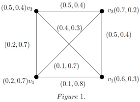
Here, let be an IF-geodetic convex set since . Similarly, and are IF-geodetic convex sets. The IF-geodetic eccentricity of a vertex is = . Also, = 0.25 and = 0.45.
The observations mentioned in the following proposition pass for obvious.
Proposition 1.
Let = be an IFG. Then the set of entire vertices, all singleton sets of vertices, and the null set are IF-geodetic convex.
Theorem 1.
For an IFG = , the intersection between two IF-geodetic convex sets is again IF-geodetic convex.
Proof.
Let’s assume ∈, we observe that both and are in X and Y. This leads to the desirable conclusion, that all the vertices in each IF-geodesics are both in X and Y.Therefore, is an IF-geodetic convex. □
Theorem 2.
If = be an IF-tree, there exists an IF-spanning subgraph and has a finite collection of nested sets = where each is IF-geodetic convex.
Proof.
Assume that is an IF tree, from the definition, there is an IF spanning subgraph, say = and which is a tree. Since is a tree, it assures the existence of a single path between any pair of vertices. This leads us to an important observation, that each path connecting any pair of vertices is a unique IF-geodesic. Thus the union of all vertices in every geodetic path is an IF-geodetic convex. Let be a subgraph of that is obtained from the set by removing a terminal vertex from . As a result, IF-subgraph is a tree. Similar justifications lead us to the conclusion that is an IF-geodetic convex. We keep going till we obtain a singleton set. Thus, it is undeniably true that the finite collection of nested sets exists in a manner that allows for = . □
4. Algorithm to Compute Geodetic Path of IFGs
Let = be an IFG with n vertices. In the literature of graph theory, various algorithms are available to compute the geodetic path between pairs of nodes. In this part, we created an algorithm for determining the geodetic path of an intuitionistic fuzzy graph and, more specifically, we offered a Python program initially for identifying all geodetic paths of IFGs.
4.1. Python Program for Identifying All Geodetic Paths of IFGs
# A program to find Geodetic Paths in an IFG
vertices = str(input("Enter the vertices : "))
# we will take all the vertices in graph
vertices = vertices.split("_")
def path_finder(vertices):
"""Find all the possible source-destinations"""
ver1 , ver2 = vertices, vertices
paths = []
for v in ver1:
for v_ in ver2:
if v != v_:
path_ = str(v)+"_"+str(v_)
if path_ in paths or str(v_)+"_"+str(v) in paths:
pass
else:
paths.append(path_)
#print(paths)
return paths
source_dest = path_finder(vertices)
PATH_SUBPATHS = {} # store source-destination : [path1,path2,path3...]
for src_des in source_dest:
v1,v2 = src_des.split("_")
print("Please enter the no of possible paths between ’{v1}’ and ’{v2}’
".format(v1 = v1, v2 = v2 ))
no_path = int(input(":=> "))
sub_path_list = []
for i in range(no_path):
sub_path = str(input("Enter path {path} : ".format(path = i )))
sub_path_list.append(sub_path)
PATH_SUBPATHS[src_des] = sub_path_list
print(PATH_SUBPATHS)
CALCULATED_PATHS = {} #{MAIN_PATH1:{PATH:distance},
MAIN_PATH2 : {PATH:distance}}
class Distance:
"""A class for distance calculation"""
def __init__(self):
pass
def get_weight(self,mu2,gama2):
weight = (1+mu2-gama2)/2
return weight
def distance(self,path):
no_edges = len(path.split("_")) - 1
weight_sum = 0
print("Enter the edges of subpath "+ path + " accordingly")
for i in range(no_edges):
edge = input("Enter the edge "+ str(i+1) + " : ")
edge = tuple(float(num) for num in edge.split())
weight = self.get_weight(mu2 = edge[0], gama2 = edge[1])
weight_sum += weight
return weight_sum
for MAIN_PATH in PATH_SUBPATHS.keys():
paths_mainpath = PATH_SUBPATHS[MAIN_PATH]
dist = Distance()
CALCULATED_PATHS[MAIN_PATH] = {}
for path in paths_mainpath:
CALCULATED_PATHS[MAIN_PATH][path] = dist.distance(path)
print(CALCULATED_PATHS)
FINAL_GEODETICS_PATHS = {} #{MAIN_PATH:{"GEODESIC_PATH":value}}
for MAIN_PATH in CALCULATED_PATHS.keys():
distances = list(CALCULATED_PATHS[MAIN_PATH].values())
keys = list(CALCULATED_PATHS[MAIN_PATH].keys())
min_distance = sorted(distances)[0]
min_index = distances.index(min_distance)
Gdesic_path = keys[min_index]
FINAL_GEODETICS_PATHS[MAIN_PATH] ={}
FINAL_GEODETICS_PATHS[MAIN_PATH][Gdesic_path] = min_distance
print(====================GEODESIC PATHS======================)
print(FINAL_GEODETICS_PATHS)
4.2. Algorithm
- Step 1. Determine how many vertices there are in the graph.
- Step 2. Identify the number of possible pathways between each pair of nodes.
- Step 3. Make a list of all possible pathways for each source and destination vertices.
- Step 4. Using the Python program to locate geodetic paths from the paths mentioned in Step 3. Enter the edge values of the sub-paths accordingly.
- Step 5. A distance class will be constructed using a predetermined distance formula.
- Step 6. Construct an matrix , where each row and column represent the vertices in IFG. If row i corresponds to vertex ui and column j corresponds to vertex , then the appropriate element in the array is = .
- Step 7. Obtain a list of every geodetic path and its associated distance between two vertices. So, in Step 7, we are able to obtain all of the geodetic pathways.
5. Intuitionistic Fuzzy Geodetic Blocks
In intuitionistic fuzzy graphs, the idea of blocks was established by Muhammad Akram and N. O. Akshehri in 2014. In this section, we present the notion of intuitionistic fuzzy geodetic blocks and some of its characterization.
Definition 8.
A connected intuitionistic fuzzy subgraph of is called an intuitionistic fuzzy geodetic block (IFGB) if there doesn’t exists a path such that .
A fact that should be evident from the definition is that in an IFGB there is only one IF-geodetic path between any pair of nodes. For a complete IF-subgraph, the edges themselves act as sole IF-geodetic path.
Example 2.
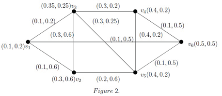
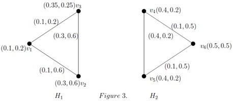
To familiarize ourselves with Definition 8, let’s consider an IFG in above Figure 2 and its subgraphs in Figure 3. Here the IF-subgraph is an IFGB. But on the other hand is not an IFGB, since there exist more than one IF-geodetic paths in between the vertices and .
Theorem 3.
If = be a complete IF-subgraph of a connected IFG . Then is an IFGB if and only if is IF-geodetic convex for any .
Proof.
Let = represent a connected IFG and = be a complete IF-subgraph of . For the forward direction, we begin with the assumption that is an IFGB. Since it is an IFGB and complete, every edge that connects two vertices serves as the only IF-geodetic path. This shows that is IF-geodetic convex.
To prove the other half of the theorem, suppose that is IF-geodetic convex for any . To prove there is only one IF-geodetic path between any pair of nodes, we assume for contradiction that there exists another IF-geodesic in , say . Suppose that has m edges. Infact, is complete, thus will exceeds , but which is not possible. This contradiction finishes the proof. □
Theorem 4.
Let = be a complete IF-subgraph of a connected IFG . If is an IFGB, then is an IF-geodetic convex.
Proof.
Let = be a complete IF - subgraph of a connected IFG . Since is an IFGB, there doesn’t exists a path in such that . Here, in this case is complete, leads to the conclusion that an edge connecting any pair of vertices in itself is the only IF -geodesic between them. Thus, the vertices in all IF geodesics are exactly and . This is obvious for any pair of vertices in , hence we are done. □
Theorem 5.
If a complete IF-subgraph of a connected IFG is an IFGB. Then every vertex removed IF-subgraph of an IFGB generates an IFGB again.
Proof.
Assume that = is an IFGB and a complete IF-subgraph of a connected IFG . Let and be the vertex removed IF-subgraph of generated by . Since is complete,leads to the conclusion that an edge linking any two vertices is the single IF-geodesic between them. As a result, removing any vertex has no effect on any IFGB property. This completes the proof. □
6. Geodetic Intuitionistic Fuzzy Boundary and Internal Vertices
In this section, the IF-boundary and IF-internal vertices of IF-geodetic convex sets are expounded. Let’s first state the relevant definition, and then look at some examples before their features are get examined.
Definition 9.
Given a connected IFG = and ρ be a non-empty subset of , which is an IF-geodetic convex. A node is called a Geodetic IF-boundary vertex of ρ if is an IF-geodetic convex. Otherwise, is referred to as a Geodetic IF-internal vertex of ρ.
Example 3.
Consider an IFG exhibited in Figure 4.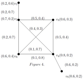
Observe that the direct edge is an IF-geodesic and the path is an IF geodesic. At this point, we let and which is an IF-geodetic convex, since . Similarly, is an IF-geodetic convex. Now we have is an IF-geodetic convex, vertex is a geodetic IF-boundary vertex of ρ. But vertex is a geodetic IF-internal vertex.
Example 4.
Looking back at our Example 1, is an IF-geodetic convex. Similarly, and are IF-geodetic convex. Here, the vertices and are geodetic IF-boundary vertices.
The following theorems are devoted to characterizing geodetic IF- boundary and geodetic IF- internal vertices.
Theorem 6.
Given any set of a connected IFG, and ρ be an IF-geodetic convex. Then a vertex is a geodetic IF-boundary vertex of ρ if and only if doesn’t cite on any IF-geodesic for all .
Proof.
Let of a connected IFG be an IF-geodetic convex. Assume that is a geodetic IF-boundary vertex of ρ and . Since is a geodetic IF-boundary vertex of ρ, we have is an IF-geodetic convex. By Definition 4, all the vertices in all IF-geodesics together with and are contained in . This implies all IF-geodesics are not dependent on . Hence doesn’t cite on any IF-geodesic for all .
For the reverse implication, suppose that doesn’t cite on any IF-geodesic for all . We show that is a geodetic IF-boundary vertex. Definition 9 insists that it is enough to establish that is an IF-geodetic convex. By hypothesis, all IF-geodesics are independent from . Notice that, , therefore all the vertices in an IF-geodesic connecting any two vertices of are contained in . Hence we are done. □
Theorem 7.
Given any set of a connected IFG, and ρ be an IF-geodetic convex. Then a vertex is a geodetic IF-internal vertex of ρ if and only if is sited in at least one IF-geodesic for some .
Proof.
Let be a geodetic IF-internal vertex of ρ and . Since is a geodetic IF-internal vertex, the set fails to be an IF-geodetic convex. By Definition 4, there exists at least one node in any of the IF-geodesics that is not a member of . Moreover, we observe that . This leads to the conclusion that is a part of at least one IF-geodesic.
For the converse statement, we may assume that lies on a IF-geodesic for some . Now it is just a matter of examining that is a geodetic IF-internal vertex of ρ. It is sufficient, if we show that fails to be an IF-geodetic convex. We begin by observing that the set , which is an IF-geodetic convex. By hypothesis, there is a presence of at least one IF-geodesic which contains . Hence the set is not an IF-geodetic convex, as desired. □
Theorem 8.
Let = be a complete IF-subgraph of = . If = is an IFGB, then every node of is a geodetic IF-boundary vertex of .
Proof.
Assume that is an IFGB. Let be any node in . In order to show is a geodetic IF-boundary vertex of , it suffices to prove is IF-geodetic convex. By Theorem 3, is an IF-geodetic convex for any . Since is arbitrary, it leads to our desired conclusion. □
7. Minimal IF-Geodetic Subgraph
There is no end to the remarkable characteristics of the IF geodesics. The introduction to the geodetic IF-cover, geodetic IF-basis, and geodetic IF-number of an IFG is the primary focus of this section. We introduce the idea of the minimal IF-geodetic subgraph in IFGs and its characterizations are presented.
Definition 10.
A subset ρ of in a connected IFG = is said to be a geodetic IF-cover of if .
Definition 11.
A Geodetic IF-Basis for = is any of with the fewest vertices, and the number of vertices in it is termed as the geodetic IF-number and denoted by .
Example 5.
To become acquainted with the above definition, let’s consider = as in Figure 5. Here the path is an IF geodesic. Let , then , so is an and observe that . Also serves the role of an .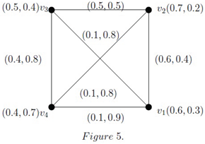
Theorem 9.
In a complete IFG, the full set of vertex is the only of .
Proof.
For a complete IFG, each edge between a pair of vertices acts as the sole IF-geodetic path. Hence, the theorem is obvious. □
An immediate corollary to Theorem 9 is as follow:
Corollary 1.
For a complete IFG , .
Theorem 10.
If = is an IF-tree, there exists an IF-subgraph that spans a unique consisting of its end nodes.
Proof.
An observation that should be immediately evident from Theorem 2, there exists an IF spanning subgraph and has a finite collection of nested sets that are IF geodetic convex. By construction of such a finite collection, it guarantees that there exists a unique for consisting of its end vertices. □
Based on the definitions and as well as the findings presented thus far, lower and upper bounds for the can be determined as follows.
Theorem 11.
Consider any non-trivial IFG with n vertices, .
Proof.
In a non-trivial IFG , of has to consist of at least two vertices in it and thus, . Also, full vertex set of is an of , clearly . This completes the proof. □
Definition 12.
An IF-graph = is called a minimal IF-geodetic subgraph if there exists an IF-graph containing such that .
Example 6.
To get a sense of the above definition, let’s once again take a look into the Figure 5 in Example 5 and here, we consider IF-subgraph = of given in Figure 6.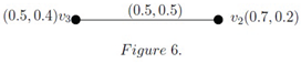
Clearly = a minimal IF-geodetic subgraph of , since, , then , so is an and at the same time with . Here,, and . Therefore, and are geodetic IF- peripheral vertices of .
The next theorem holds for obvious reasons.
Theorem 12.
Let = be a minimal IF-geodetic subgraph of with , then are geodetic IF- peripheral vertices of .
Theorem 13.
If = with n vertices, .
Proof.
Let = be a non-trivial IF-subgraph of with the number of vertices equal to . Then, using Theorem 11, it is apparent that . Since, by hypothesis, is a minimal IF-geodetic subgraph of , . Thus,, we conclude that . Again, by Theorem 7.7, it is clear that . □
The next theorem should be compared with Theorem 9 and Corollary 1.
Theorem 14.
The only minimal IF-geodetic subgraph of the complete IFG is itself.
Proof.
To argue for this, we use Theorem 9. For a complete IFG, each edge between pair of vertices acts as sole IF-geodetic path. Hence, is the entire set of vertex. Therefore, , which completes the proof. □
8. Intuitionistic Fuzzy Geodetic Wiener Index
The Wiener index is a well-known index that is utilized in a variety of sectors such as telecommunication, facility localization, chemical graphs, networking and so on. A connected IFG accurately models a wide range of circumstances. This section introduces the notion of the Intuitionistic Fuzzy Geodetic Wiener Index () using the IF-geodesics, and the formal formulation is as follows.
Definition 13.
If : is a path in an IFG, the Intuitionistic Fuzzy Geodetic Wiener Index is defined as = where is the IF-geodetic distance from to .
Example 7.
Let = be an IFG (Figure 1). The direct edges , and are IF-geodesics. The paths , and are IF-geodesics. Here, = .
Removing a node from a graph usually creates a subgraph of the original graph. As a result, the type of graph determines whether will increase, decrease, or remain constant. In most cases, the index will decrease. The effect of removing a bridge on will be discussed in the upcoming scenario.
Example 8.
In Figure 7 the path and have the strength and , respectively. Here, the edge that joins and serves as both a bridge and a geodesic. In this case = 2.2, but = 2.25.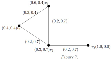
The above case will be generalized by the following theorem.
Theorem 15.
If a bridge is removed from an IFG, then increases only if it is an edge of any geodesic.
Proof.
Assume that there exist a bridge in an IFG, say . Now we consider two possibilities as follows. Case 1: Suppose that itself a geodesic for some i and j. Then, . Thus deletion of will increase the value of . Hence from the definition of , we are done. Case 2: Take as an edge of any geodetic path joins any pair of vertices. Since the deletion of creates new geodetic path.Thus there will be an increase in . □
Theorem 16.
The of two isomorphic IFGs are equal.
Proof.
Let = and = be two isomorphic IFGs. Then there exists a bijective map such that for every and and . Similarly, for every there exists . As a result, we can categorically state that there is a path in that corresponds to the path in such that the sum of weights of edges is minimum among all the paths from . Hence = . Therefore, = = = = = , as desired. □
9. Applications
9.1. Application of in Wireless Mesh Network
In 2015, mesh networking for small networks made its debut with the promise of resolving Wi-Fi issues through increased coverage, faster networks, and less fuss. In order to prevent inactive and weak spots, it also claimed to eliminate the requirement for base stations to be placed precisely across a house or small workplace. Mesh networks also offer help in figuring out where to locate units. Mesh networks have the ability to scale effortlessly by incorporating additional nodes without requiring substantial alterations to the network infrastructure, making them well suited to extend coverage over expansive areas. In general, wireless mesh networks provide a robust and decentralized networking solution that is applicable in numerous scenarios where traditional wired networks are not viable or feasible.
For instance, in a University campus environment, setting up a wireless mesh network can help increase network coverage and efficiency. Every node in a wireless mesh network communicates with other nodes in the area, creating a scalable and self-healing network. For stability and to prevent wireless congestion, certain nodes could still require a wired Ethernet connection to the main router to accomplish this. In order to plan and configure a wireless mesh network (WMN), follow these general steps. The first step is to survey the area, where we identify areas that need Wi-Fi coverage and make note of any obstacles such as walls and other structural constraints. The second factor, node location, guarantees that the wireless mesh is strategically placed and that the entire region is adequately covered. Lastly, the types of node are crucial in designating specific nodes as "gateway" nodes that provide a direct Ethernet connection to the main router. The remaining nodes will be "mesh" nodes that establish wireless connections with both the gateway and other nodes. Use Ethernet connections to link gateway nodes to the main router. In a wireless mesh network, not all nodes necessarily need a wired connection. We need to identify gateway nodes, or the nodes that need to be linked to the cable in order to cover the entire area. With the help of geodetic IF-cover, we can now tackle the issue. To make computations easier, we have taken . Take a look at the fuzzified WMN model shown in Figure 8.
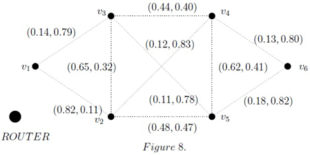
Here we have, 16 geodetic pathways in total, in particular consider the pathway, : is an IF geodesic and = 0.83, likewise, : is an IF - geodesic. Let , then , so is an for the WMN mentioned above. Consequently, we may identify and as our gateway nodes, enabling them to cover the whole region of the network. Here act as as well. The following Figure 9 depicts the finalized structure of a wireless mesh network, where gateway nodes are highlighted in red, mesh nodes are identified with green labels, dotted lines in the figure symbolize wireless connections, while solid lines without breaks indicate wired connections with the router.
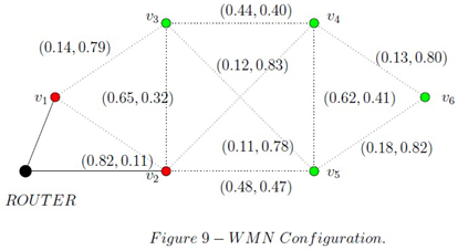
Note that depending on the hardware and software solutions you select for your wireless mesh network, there may be differences in the precise processes and required equipment. For the finest implementation, it is also a good idea to speak with network or IT specialists. More coverage, better connectivity, and an increase in total network capabilities can be achieved by expanding and improving a WMN to create a more complex and sophisticated network configuration.
9.2. Application of in Global Human Trading
Human trading often involves intricate networks of individuals and organizations. Taking into account the ambiguity and uncertainty in the connections, IFG theory can be used to examine and visualize these networks. Law enforcement and policymakers may find this analysis useful in understanding the dynamics and structure of trafficking networks. In this paper, we use the major illegal human trade routes to the United States as mentioned in [3,6].
Several approaches were applied to fuzzy graphs to assess the likelihood of illegal immigration along various routes from the countries of origin to the United States. In this study, we quantify the susceptibility to trafficking with respect to a directed IFG using . We interpret as flow from distinct locations and represents government measures to control internal transit fluxes. Consider Figure 11 in [9] as a model of directed IFG. Thus, Table 1 can be constructed as follows.
It is important to emphasize that the Wiener indices fall as the effectiveness of a path in preventing trafficking rises. Consider the path from India to U.S., = = 0.265 + 0.325 + 0.47 = 1.06. Using analogous computations along the path from Somalia to our desired destination reveals two distinct pathways. One is through Guatemala with is 3.485 and the other one is directly through Mexico from Colombia and its index is 1.745. An of 1.37 linked to the route originating from China as the country of origin. Along Nigeria to U.S via Guatemala, =2.04. Directly traversing the route via Colombia through Mexico to the United States from country origin Nigeria registered an of 1.6. It has been determined that along the path from Ethiopia, there is an of 1.84.
Measures of a route’s vulnerability to illegal human trading are established by applying the principles and results. One potential such metric is the , which is introduced.Three techniques were employed in fuzzy graphs to assess the likelihood of illegal immigration along certain routes from the countries of origin to the United States. The method in this research and the other methods in article [3,6,9] concur that the path leading to the United States with the highest susceptibility originates in Somalia. The source nation with the second-highest likelihood is Nigeria. The newfound method proves to be more accurate, as it takes into account internal transit flow. Upon comparing the average Wiener index in fuzzy graphs with the indexes obtained in this paper, it can be concluded that this method is more precise and accurate.
10. Conclusions
A notion of intuitionistic fuzzy geodetic convexity within the framework of intuitionistic fuzzy graph metric is discussed in this article. This paper culminated in the development of a specialized algorithm for identifying the geodetic path of an IFG. Also we presented a Python program crafted for the precise identification of all geodetic paths. This article is devoted in the development of IF-boundary vertices, IF-internal vertices, geodetic IF-basis and geodetic IF-number within IF-geodetic convex sets. A lower and upper bounds for the geodetic IF-number is also identified in this article. Later, we introduced the idea of the minimal IF-geodetic subgraph in IFGs. We introduced a novel concept, the intuitionistic fuzzy geodetic Wiener index, leveraging the framework of IF-geodesics. Finally, the application of IF-geodetic cover in a wireless mesh network for identifying gateway nodes. Additionally, the introduction of the intuitionistic fuzzy geodetic Wiener index has found practical application in the domain of global human trading analysis in certain trafficking channels to the U.S. The findings coincide with those reported in earlier studies.
Author Contributions
Conceptualization, A.M.A., R.R., L.E.P and V.M.M.R.; methodology, A.M.A., R.R and L.E.P; writing—original draft preparation, A.M.A., R.R. and L.E.P; writing—review and editing, A.M.A., R.R., L.E.P and V.M.M.R.; supervision, A.M.A. All authors have read and agreed to the published version of the manuscript.
Funding
This research received no external funding.
Data Availability Statement
The original contributions presented in this study are included in the article. Further inquiries can be directed to the corresponding author.
Acknowledgments
The authors would like to thank the reviewers for their valuable suggestions in improving the quality of this paper.
Conflicts of Interest
The authors of this paper declare that they have no conflicts of interest.
References
- Rosenfeld, A. Fuzzy graphs. In Fuzzy Sets and Their Applications; Academic Press: New York, NY, USA, 1975; pp. 77–95. [Google Scholar]
- Atanassov, K.T. In: Intuitionistic fuzzy sets: theory and applications. Physica, NewYork.
- Darabian, E.; Borzooei, R.A. . Results on vague graphs with applications to human trafficking. New Math. Nat. Comput. 2018, 14, 37–52. [Google Scholar] [CrossRef]
- Gary Chartrand; Gamy, L. J.; Songlin Tian. Detour Distance in Graphs. Annals of Discrete Mathematics. 1993, 55, 127–136. [Google Scholar]
- Mordeson, J.N.; Nair, P.S. Fuzzy Graphs and Fuzzy Hypergraphs; Physica: Heidelberg, Germany, 2012. [Google Scholar]
- Mordeson, J.N.; Mathew, S. t-Norm fuzzy graphs. New Math. Nat. Comput. 2018, 14, 129–143. [Google Scholar] [CrossRef]
- Mordeson, J.N.; Mathew, S. Advanced Topics in Fuzzy Graph Theory; Springer International Publishing: 2019.
- Akram, M.; Davvaz, B. Strong intuitionistic fuzzy graphs. Filomat. 2012, 26, 177–196. [Google Scholar] [CrossRef]
- Binu, M.; Mathew, S.; Mordeson, J.N. Wiener index of a fuzzy graph and application to illegal immigration networks. Fuzzy Sets Syst. 2020, 384, 132–147. [Google Scholar]
- Karunambigai, M.G.; Parvathi, R.; Buvaneswari, R. Arcs in intuitionistic fuzzy graphs. Notes on Intuitionistic Fuzzy Sets. 2011, 17, 37–47. [Google Scholar]
- Nagoor Gani, A.; Radha, K. On Regular Fuzzy Graphs. Journal of Physical sciences. 2008, 12, 33–40. [Google Scholar]
- Nagoor Gani, A.; Shajitha Begum, S. Degree, Order and Size in Intuitionistic Fuzzy Graphs. International Journal of Algorithms, Computing and Mathematics. 2010, 3. [Google Scholar]
- Nagoor Gani, A.; Akram, M.; Anupriya, S. Degree, Double domination on intuitionistic fuzzy graphs. Journal of Applied Mathematics and Computing . 2015, 52. [Google Scholar]
- Parvathy, R.; Karunambigai, M.G. Intuitionistic Fuzzy Graphs. Computational Intelligence, Theory and applications; Springer: Berlin, Heidelberg, 2006; pp. 139–150. [Google Scholar]
- Rajeshkumar, R.; Anto, A.M. Some domination parameters in intuitionistic fuzzy graphs. AIP Conf. Proc. 2022, 2516, 200016. [Google Scholar]
- Rajeshkumar, R.; Anto, A.M. Fuzzy Detour Convexity and Fuzzy Detour Covering in Fuzzy Graphs. Turkish Journal of Computer and Mathematics Education. 2021, 12, 2170–2175. [Google Scholar]
- Mathew, S.; Mordeson, J.N.; Malik, D.S. Fuzzy Graph Theory; Springer International Publishing: 2018.
- Sunitha, M.S.; Vijayakumar, A. Complement of a fuzzy graph. Indian Journal of Pure and applied Mathematics. 2002, 33, 1451–1464. [Google Scholar]
- Mohamed, S.Y.; Mohamed Ali, A. Intuitionistic Fuzzy Graph Metric Space. International Journal of Pure and Applied Mathematics. 2018, 118, 67–74. [Google Scholar]
- Naeem, T.; Gumaei, A.; Kamran Jamil, M.; Alsanad, A.; Ullah,K. Connectivity Indices of Intuitionistic Fuzzy Graphs and Their Applications in Internet Routing and Transport Network Flow. Mathematical Problems in Engineering. 2021, 2021, 4156879. [Google Scholar] [CrossRef]
- Zadeh, L.A.; Fu, K.S.; Shimura, M. Fuzzy sets and their applications; Academic Press: 1975; pp. 125-149.
- Zadeh, L.A. Fuzzy sets. Information and Control. 1965, 8, 338–353. [Google Scholar] [CrossRef]

| Country | Vulnerability ( ) | Government Measure() | () | () |
|---|---|---|---|---|
| India | 0.46 | 0.53 | 0.26 | 0.73 |
| China | 0.36 | 0.45 | 0.19 | 0.68 |
| Russia | 0.3 | 0.42 | 0.06 | 0.61 |
| UAE | 0.56 | 0.26 | 0.17 | 0.57 |
| Somalia | 0.28 | 0.72 | 0.16 | 0.79 |
| Ethiopia | 0.42 | 0.58 | 0.21 | 0.79 |
| South Africa | 0.49 | 0.49 | 0.32 | 0.65 |
| Nigeria | 0.44 | 0.56 | 0.31 | 0.65 |
| Spain | 0.71 | 0.2 | 0.15 | 0.46 |
| Cuba | 0.21 | 0.32 | 0.11 | 0.61 |
| Colombia | 0.53 | 0.42 | 0.30 | 0.66 |
| Brazil | 0.66 | 0.31 | 0.34 | 0.55 |
| Ecuador | 0.51 | 0.35 | 0.29 | 0.63 |
| Guatemala | 0.56 | 0.42 | 0.3 | 0.67 |
| Mexico | 0.57 | 0.43 | 0.47 | 0.53 |
| United States | 0.82 | 0.18 | 0 | 0 |
Disclaimer/Publisher’s Note: The statements, opinions and data contained in all publications are solely those of the individual author(s) and contributor(s) and not of MDPI and/or the editor(s). MDPI and/or the editor(s) disclaim responsibility for any injury to people or property resulting from any ideas, methods, instructions or products referred to in the content. |
© 2025 by the authors. Licensee MDPI, Basel, Switzerland. This article is an open access article distributed under the terms and conditions of the Creative Commons Attribution (CC BY) license (http://creativecommons.org/licenses/by/4.0/).
Copyright: This open access article is published under a Creative Commons CC BY 4.0 license, which permit the free download, distribution, and reuse, provided that the author and preprint are cited in any reuse.


