
Submitted:
29 April 2025
Posted:
19 May 2025
You are already at the latest version
Abstract
Outlier testing and elimination can be avoided via application of robust estimators. Amongst robust estimators, the Q/Hampel method displays the best performance (in terms of breakdown point and efficiency). While the formulas and correction factors for Q/Hampel in the case of the design with two variance components (e.g. within- and between-laboratory variance) have already been made available, corresponding formulas for other designs have not. A case in point is the staggered-nested design, which is a highly efficient design for e.g. the estimation of intermediate precision in method validation studies. Accordingly, the formulas and correction factors for the use of Q/Hampel in the staggered-nested design are provided here.
Keywords:
interlaboratory study
; staggered-nested design
; reproducibility precision
; intermediate precision
; robust estimator
1. Introduction
In the case of quantitative methods, the aim of interlaboratory validation studies is to characterize method performance in terms of trueness and precision. ISO 5725-2/-3/-4 ([1], [2], [3]) provide a number of different designs allowing the evaluation of these two performance characteristics.
A particularly powerful design is the staggered-nested design described in ISO 5725-3 [2]. The simplest such design is the two-factor staggered-nested design, where each laboratory obtains three test results. For laboratory , test results and are obtained under repeatability conditions, and under intermediate conditions, e.g. on a different day.
The standard calculation method for precision is analysis of variance (ANOVA), preceded by outlier testing. While ANOVA, under the normal distribution assumption, is very efficient in the case of balanced designs, in the case of unbalanced designs, such as the staggered-nested design, the usual ANOVA does not use all the information available in the data. This is related to the fact that the reproducibility standard deviation is not calculated directly, but rather from the laboratory and intermediate standard deviation values; while the latter, in turn, is calculated from the standard deviation under intermediate conditions and the repeatability standard deviation. Another disadvantage of ANOVA and other conventional methods is that they very much depend on the data following a normal distribution and are thus highly sensitive to outliers. This can only be partially offset via outlier tests, since even if conspicuous values are not yet statistically significant outliers, considerable deviations can result in the determined precision data.
The advantage of robust estimators is that no outlier testing is required. For the estimation of means and standard deviation values, different robust estimators exist. The performance of a given robust estimators can be characterized via breakdown point (proportion of data that can be outliers without the estimate being affected) and efficiency (ratio of the statistical uncertainty of the estimate to that of the classical estimator under the normal distribution assumption). An overview of different breakdown point and efficiency values is provided in ISO 13528 [4].
The Q/Hampel and Qn methods have both the highest breakdown point and the best efficiency.
The Q/Hampel method uses the Q method for the calculation of the robust reproducibility standard deviation and repeatability standard deviation together with the Hampel estimator for the calculation of the location parameter as described in ISO 13528 [4]. The theoretical basis for the Q method, including asymptotic performance and finite sample breakdown, is described in Müller et al. [5] and Uhlig [6].
The Q method is not only robust against outlying results, but also against a situation where many test results are identical, e.g. due to quantitative data on a discontinuous scale or due to rounding distortions. In such a situation other Q-like methods (e.g. the Qn method originally introduced by Rousseeuw et al. [8] for univariate data) can fail because many pairwise differences are zero.
The Q method was introduced for the one-way random effect model and later modified – for ISO 13528 [4] – to deal with the situation that that there are many equal data, e.g., for the case where the number of significant digits is too small.
The Q/Hampel method is typically used for conventional designs, but it can also be applied for the staggered-nested design with two factors according to ISO 5725-3 [2] – in particular for estimating the intermediate standard deviation in addition to the reproducibility and repeatability standard deviation.
2. Robust Statistical Analysis of Results by Means of the Q/Hampel Method in a Staggered-Nested Design with Two Factors
For each level, the data obtained in the experiment are denoted (with representing factor 0, i.e. laboratory, ; representing factor 1, ; and representing the replicate, with ranging from to , with and ), i.e. for laboratory there are three measurement results , , In summary, test results, grouped by laboratory, are denoted as follows:
2.1. Determination of the Robust Reproducibility Standard Deviation
Using the Q Method
The calculation relies on the use of pairwise differences within the data set and, thus, does not depend on the estimate of the mean or median.
The algorithm can be described as follows.
Based on the measurement results as structured in equation (1), the cumulative distribution function of all absolute between-laboratory differences is calculated as follows:
where denotes the indicator function.
Discontinuity points of are denoted
For each positive discontinuity points , define
and let
For each within the interval , is obtained by linear interpolation between discontinuity points .
Finally, the robust reproducibility standard deviation is obtained as
where is calculated as in equation (2) and is set equal to zero unless there are identical values in the data set.
In Equation (4), denotes the quantile of the standard normal distribution and denotes the correction factor corresponding to the number of laboratories .
The correction factors were obtained via a simulation study, which will now be briefly described. In each simulation step, normally () distributed data corresponding to laboratories were generated and the robust reproducibility standard deviation was calculated in accordance with the Q method from the formulas given above. Taking the mean value across simulation steps – separately for each – it was possible to calculate the expected value for the reproducibility standard deviation . For a given , the correction factor was then obtained by taking the reciprocate of the expected value. For each value between 4 and 100, Table 1 provides the expected value for the reproducibility standard deviation along with the corresponding relative standard error and correction factor .
For , it was possible to derive a functional relationship between and the correction factor via nonlinear optimization. This functional relationship is given in equation (5) and presented in Figure 1 for .
2.2. Determination of the Robust Intermediate Standard Deviation Using the Q Method
Take the case that factor 1 is day. As explained above, in the two-factor staggered-nested design, there are two results for day 1, and one for day 2. For a given laboratory, there are thus two within-laboratory differences corresponding to factor 1. Accordingly, the cumulative distribution function corresponding to factor 1 is calculated as follows:
where denotes the indicator function.
As above, the discontinuity points of are denoted
For each positive discontinuity points , define
and let
For each within the interval , is obtained via linear interpolation between discontinuity points .
Finally, the robust intermediate standard deviation is obtained as
where is calculated as in equation (6) and is set equal to zero unless there are identical values in the data set.
As above, denotes the quantile of the standard normal distribution.
Similarly to in the previous section, for a given number of laboratories , the correction factor was calculated via a simulation study.
For each value between 4 and 100, Table 2 provides the expected value for the intermediate standard deviation along with the corresponding relative standard error and correction factor .
For , it was possible to derive a functional relationship between the number of laboratories and the correction factor via nonlinear optimization. The functional relationship for is given in equation (9) and shown in Figure 2.
If results in a value greater than , then is set to .
2.3. Determination of the Robust Repeatability Standard Deviation
Using the Q Method
As far as repeatability is concerned, there is only one difference which can be calculated per laboratory in the two-factor staggered-nested design: namely, that corresponding to the this first level of factor 1 (e.g. the two results obtained on day 1, if factor 1 is day). Accordingly, the cumulative distribution function corresponding to repeatability precision is calculated as follows::
where denotes the indicator function.
As above, the discontinuity points, the discontinuity points of are denoted
For each positive discontinuity points , define
and let
For each within the interval , the function is calculated via linear interpolation between discontinuity points .
Finally, the robust repeatability standard deviation is obtained as
where is calculated as in equation (10) and is equal to zero unless there are identical values in the data set.
As above, denotes the quantile of the standard normal distribution.
The correction factor is the same as in the previous section, see Table 2 and equation (9).
If is greater than , then is set equal to .
2.4. Determination of the Robust Mean
Using the Hampel Estimator
Calculate the weighted means for each laboratory, denoted , i.e.
Calculate the robust mean, , by solving the equation
where
and
where , and denote the robust reproducibility, intermediate and repeatability standard deviations obtained in accordance with the Q method (as described in 2.1, 2.2 and 2.3), respectively.
The exact solution may be obtained in a finite number of steps (not iteratively) using the property that is partially linear in and by means of the interpolation nodes of the left side of equation (14) (interpreted here as a function of ).
The interpolation nodes are obtained as follows
- for the first value :
, , , , ,
- for the first value :
, , , , ,
- and so on for all values .
The notes are sorted in ascending order: .
For each , the following quantity is then calculated:
It is then checked whether
. If so, is a solution of equation (14).
. If so, is a solution of equation (14).
. If so, is a solution of equation (14).
Let denote the set of all solutions of equation (14).
The solution nearest to the median is taken as the location parameter , i.e
Several solutions may exist. If there are two solutions nearest the median, or if there is no solution at all, the median itself is taken as the location parameter .
This implementation of Hampel’s estimator has approximately 96 % efficiency for normally distributed data.
If this estimation method is used, laboratory results differing from the mean by more than 4,5 times the reproducibility standard deviation no longer have any effect on the calculation result, i.e. they are treated as outliers.
3. Conclusion
The Q/Hampel procedure described in this paper extends the range of robust statistical methods to staggered-nested designs, providing for the first time an adequate approach for handling outliers in such complex experimental formats. In conventional ISO 5725 approaches, especially under unbalanced conditions, the absence of a straightforward outlier identification process at the intermediate stage often necessitates the exclusion of all results from a laboratory, resulting in significant information loss. By contrast, the robust approach presented here allows the retention of valuable data from all laboratories, maximizing the information available for the estimation of precision parameters and means. Thus, the introduction of robust estimators in staggered-nested designs ensures both the integrity of statistical analysis and the efficient use of all available data in method validation studies.
Conflicts of Interest
The authors declared no potential conflicts of interest with respect to the research, authorship, and/or publication of this article.
References
- ISO 5725-2, Accuracy (trueness and precision) of measurement methods and results — Part 2: Basic method for the determination of repeatability and reproducibility of a standard measurement method.
- ISO 5725-3, Accuracy (trueness and precision) of measurement methods and results — Part 3: Intermediate measures of the precision of a standard measurement method. -.
- ISO 5725-5, Accuracy (trueness and precision) of measurement methods and results — Part 5: Alternative methods for the determination of the precision of a standard measurement method.
- ISO 13528, Statistical methods for use in proficiency testing by interlaboratory comparisons.
- Müller, C.H. Müller C.H. and Uhlig S., Estimation of variance components with high breakdown point and high efficiency; Biometrika; 88: Vol. 2, pp. 353-366, 2001.
- Uhlig S., Robust estimation of variance components with high breakdown point in the 1-way random effect model. In: Kitsos, C.P. and Edler, L.; Industrial Statistics; Physica, S. 65-73, 1997.
- Uhlig S., Robust estimation of between and within laboratory standard deviation measurement results below the detection limit, Journal of Consumer Protection and Food Safety, 2015.
- Rousseeuw, P.J. and Croux, C., Alternatives to the Median Absolute Deviation. Journal of the American Statistical Association, 88, 1273-1283, 1993.
Figure 1.
Functional relationship between the number of laboratories and the correction factor bp for sR.
Figure 1.
Functional relationship between the number of laboratories and the correction factor bp for sR.
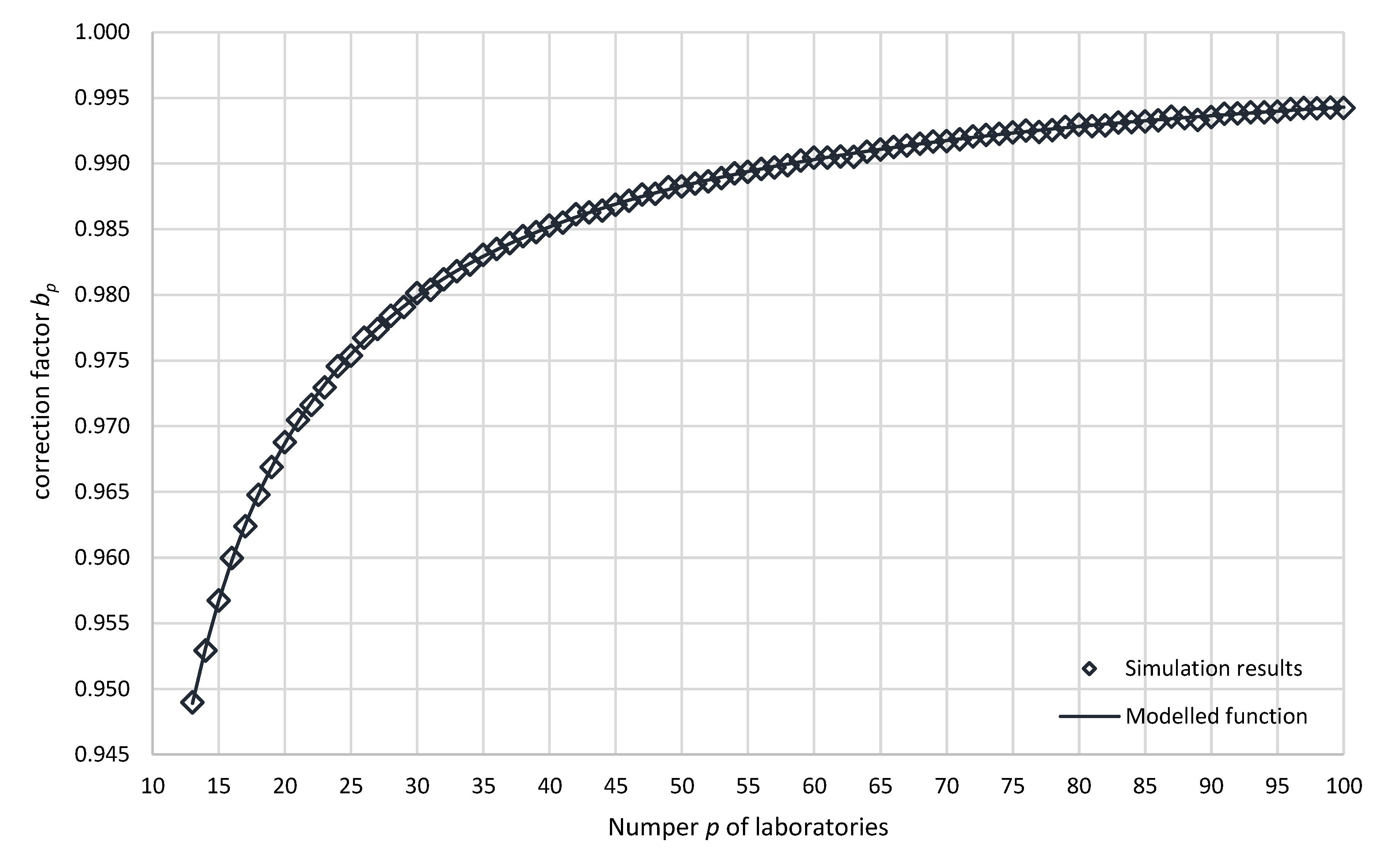
Figure 2.
Functional relationship between the number of laboratories and the correction factor for


Table 1.
Simulation results for each value of : Expected value and relative standard error for as well as the correction factor .
Table 1.
Simulation results for each value of : Expected value and relative standard error for as well as the correction factor .
| ) | ) | ) | |||||||||
|---|---|---|---|---|---|---|---|---|---|---|---|
| 4 | 1.3212 | 0.058% | 0.7569 | 37 | 1.0163 | 0.014% | 0.9839 | 70 | 1.0084 | 0.010% | 0.9917 |
| 5 | 1.1864 | 0.054% | 0.8429 | 38 | 1.0158 | 0.014% | 0.9845 | 71 | 1.0082 | 0.010% | 0.9919 |
| 6 | 1.1490 | 0.044% | 0.8703 | 39 | 1.0154 | 0.014% | 0.9848 | 72 | 1.0080 | 0.010% | 0.9921 |
| 7 | 1.1173 | 0.041% | 0.8950 | 40 | 1.0149 | 0.013% | 0.9853 | 73 | 1.0079 | 0.010% | 0.9922 |
| 8 | 1.1001 | 0.036% | 0.9090 | 41 | 1.0147 | 0.013% | 0.9855 | 74 | 1.0078 | 0.009% | 0.9922 |
| 9 | 1.0857 | 0.034% | 0.9211 | 42 | 1.0140 | 0.013% | 0.9861 | 75 | 1.0077 | 0.009% | 0.9924 |
| 10 | 1.0737 | 0.032% | 0.9313 | 43 | 1.0139 | 0.013% | 0.9863 | 76 | 1.0075 | 0.009% | 0.9925 |
| 11 | 1.0657 | 0.030% | 0.9384 | 44 | 1.0138 | 0.013% | 0.9864 | 77 | 1.0077 | 0.009% | 0.9924 |
| 12 | 1.0586 | 0.028% | 0.9446 | 45 | 1.0133 | 0.013% | 0.9869 | 78 | 1.0075 | 0.009% | 0.9925 |
| 13 | 1.0538 | 0.027% | 0.9490 | 46 | 1.0130 | 0.012% | 0.9872 | 79 | 1.0073 | 0.009% | 0.9928 |
| 14 | 1.0494 | 0.026% | 0.9529 | 47 | 1.0125 | 0.012% | 0.9876 | 80 | 1.0071 | 0.009% | 0.9930 |
| 15 | 1.0452 | 0.024% | 0.9568 | 48 | 1.0124 | 0.012% | 0.9877 | 81 | 1.0072 | 0.009% | 0.9928 |
| 16 | 1.0417 | 0.023% | 0.9600 | 49 | 1.0119 | 0.012% | 0.9882 | 82 | 1.0071 | 0.009% | 0.9929 |
| 17 | 1.0391 | 0.022% | 0.9624 | 50 | 1.0119 | 0.012% | 0.9883 | 83 | 1.0069 | 0.009% | 0.9931 |
| 18 | 1.0365 | 0.022% | 0.9648 | 51 | 1.0117 | 0.012% | 0.9885 | 84 | 1.0069 | 0.009% | 0.9931 |
| 19 | 1.0342 | 0.021% | 0.9669 | 52 | 1.0115 | 0.012% | 0.9886 | 85 | 1.0068 | 0.009% | 0.9932 |
| 20 | 1.0322 | 0.020% | 0.9688 | 53 | 1.0112 | 0.011% | 0.9889 | 86 | 1.0067 | 0.009% | 0.9933 |
| 21 | 1.0304 | 0.020% | 0.9705 | 54 | 1.0109 | 0.011% | 0.9892 | 87 | 1.0065 | 0.009% | 0.9936 |
| 22 | 1.0292 | 0.019% | 0.9716 | 55 | 1.0107 | 0.011% | 0.9894 | 88 | 1.0066 | 0.009% | 0.9935 |
| 23 | 1.0278 | 0.019% | 0.9730 | 56 | 1.0105 | 0.011% | 0.9896 | 89 | 1.0067 | 0.009% | 0.9933 |
| 24 | 1.0261 | 0.018% | 0.9746 | 57 | 1.0104 | 0.011% | 0.9897 | 90 | 1.0065 | 0.009% | 0.9935 |
| 25 | 1.0252 | 0.018% | 0.9754 | 58 | 1.0102 | 0.011% | 0.9899 | 91 | 1.0063 | 0.008% | 0.9938 |
| 26 | 1.0238 | 0.017% | 0.9768 | 59 | 1.0099 | 0.011% | 0.9902 | 92 | 1.0062 | 0.008% | 0.9938 |
| 27 | 1.0231 | 0.017% | 0.9774 | 60 | 1.0096 | 0.011% | 0.9905 | 93 | 1.0061 | 0.008% | 0.9939 |
| 28 | 1.0221 | 0.017% | 0.9784 | 61 | 1.0096 | 0.011% | 0.9905 | 94 | 1.0061 | 0.008% | 0.9939 |
| 29 | 1.0214 | 0.016% | 0.9791 | 62 | 1.0095 | 0.010% | 0.9905 | 95 | 1.0061 | 0.008% | 0.9939 |
| 30 | 1.0203 | 0.016% | 0.9801 | 63 | 1.0096 | 0.010% | 0.9905 | 96 | 1.0059 | 0.008% | 0.9941 |
| 31 | 1.0200 | 0.016% | 0.9804 | 64 | 1.0092 | 0.010% | 0.9909 | 97 | 1.0058 | 0.008% | 0.9942 |
| 32 | 1.0192 | 0.015% | 0.9812 | 65 | 1.0090 | 0.010% | 0.9911 | 98 | 1.0058 | 0.008% | 0.9942 |
| 33 | 1.0185 | 0.015% | 0.9818 | 66 | 1.0088 | 0.010% | 0.9913 | 99 | 1.0058 | 0.008% | 0.9943 |
| 34 | 1.0180 | 0.015% | 0.9823 | 67 | 1.0087 | 0.010% | 0.9914 | 100 | 1.0058 | 0.008% | 0.9942 |
| 35 | 1.0172 | 0.014% | 0.9830 | 68 | 1.0086 | 0.010% | 0.9915 | ||||
| 36 | 1.0168 | 0.014% | 0.9835 | 69 | 1.0084 | 0.010% | 0.9917 |
Table 2.
Simulation results for each value of : Expected value and relative standard error for as well as the correction factor .
Table 2.
Simulation results for each value of : Expected value and relative standard error for as well as the correction factor .
| ) | ) | ) | |||||||||
|---|---|---|---|---|---|---|---|---|---|---|---|
| 4 | 1.0855 | 0.046% | 0.9212 | 37 | 1.0081 | 0.019% | 0.9920 | 70 | 1.0043 | 0.014% | 0.9957 |
| 5 | 1.0561 | 0.046% | 0.9469 | 38 | 1.0080 | 0.018% | 0.9920 | 71 | 1.0041 | 0.014% | 0.9959 |
| 6 | 1.0550 | 0.040% | 0.9479 | 39 | 1.0077 | 0.018% | 0.9924 | 72 | 1.0043 | 0.014% | 0.9957 |
| 7 | 1.0409 | 0.040% | 0.9607 | 40 | 1.0077 | 0.018% | 0.9923 | 73 | 1.0040 | 0.014% | 0.9960 |
| 8 | 1.0410 | 0.036% | 0.9606 | 41 | 1.0074 | 0.018% | 0.9927 | 74 | 1.0041 | 0.013% | 0.9959 |
| 9 | 1.0324 | 0.036% | 0.9686 | 42 | 1.0073 | 0.018% | 0.9928 | 75 | 1.0039 | 0.013% | 0.9961 |
| 10 | 1.0321 | 0.033% | 0.9689 | 43 | 1.0072 | 0.017% | 0.9929 | 76 | 1.0040 | 0.013% | 0.9960 |
| 11 | 1.0272 | 0.033% | 0.9735 | 44 | 1.0068 | 0.017% | 0.9932 | 77 | 1.0038 | 0.013% | 0.9963 |
| 12 | 1.0270 | 0.031% | 0.9737 | 45 | 1.0064 | 0.017% | 0.9936 | 78 | 1.0040 | 0.013% | 0.9960 |
| 13 | 1.0233 | 0.031% | 0.9772 | 46 | 1.0068 | 0.017% | 0.9933 | 79 | 1.0039 | 0.013% | 0.9961 |
| 14 | 1.0231 | 0.029% | 0.9774 | 47 | 1.0066 | 0.017% | 0.9935 | 80 | 1.0038 | 0.013% | 0.9962 |
| 15 | 1.0206 | 0.029% | 0.9798 | 48 | 1.0064 | 0.016% | 0.9937 | 81 | 1.0039 | 0.013% | 0.9962 |
| 16 | 1.0200 | 0.027% | 0.9804 | 49 | 1.0064 | 0.016% | 0.9937 | 82 | 1.0034 | 0.013% | 0.9966 |
| 17 | 1.0178 | 0.027% | 0.9825 | 50 | 1.0063 | 0.016% | 0.9937 | 83 | 1.0035 | 0.013% | 0.9965 |
| 18 | 1.0173 | 0.026% | 0.9830 | 51 | 1.0057 | 0.016% | 0.9943 | 84 | 1.0037 | 0.013% | 0.9963 |
| 19 | 1.0157 | 0.026% | 0.9846 | 52 | 1.0059 | 0.016% | 0.9941 | 85 | 1.0035 | 0.013% | 0.9965 |
| 20 | 1.0157 | 0.025% | 0.9845 | 53 | 1.0058 | 0.016% | 0.9942 | 86 | 1.0036 | 0.012% | 0.9964 |
| 21 | 1.0147 | 0.025% | 0.9855 | 54 | 1.0055 | 0.016% | 0.9946 | 87 | 1.0034 | 0.012% | 0.9966 |
| 22 | 1.0140 | 0.024% | 0.9862 | 55 | 1.0053 | 0.016% | 0.9947 | 88 | 1.0036 | 0.012% | 0.9964 |
| 23 | 1.0131 | 0.024% | 0.9870 | 56 | 1.0055 | 0.015% | 0.9946 | 89 | 1.0035 | 0.012% | 0.9965 |
| 24 | 1.0134 | 0.023% | 0.9867 | 57 | 1.0052 | 0.015% | 0.9948 | 90 | 1.0036 | 0.012% | 0.9964 |
| 25 | 1.0122 | 0.023% | 0.9880 | 58 | 1.0054 | 0.015% | 0.9946 | 91 | 1.0033 | 0.012% | 0.9967 |
| 26 | 1.0121 | 0.022% | 0.9880 | 59 | 1.0050 | 0.015% | 0.9950 | 92 | 1.0034 | 0.012% | 0.9966 |
| 27 | 1.0109 | 0.022% | 0.9893 | 60 | 1.0051 | 0.015% | 0.9949 | 93 | 1.0031 | 0.012% | 0.9969 |
| 28 | 1.0112 | 0.021% | 0.9889 | 61 | 1.0052 | 0.015% | 0.9948 | 94 | 1.0032 | 0.012% | 0.9968 |
| 29 | 1.0102 | 0.021% | 0.9899 | 62 | 1.0050 | 0.015% | 0.9950 | 95 | 1.0031 | 0.012% | 0.9969 |
| 30 | 1.0102 | 0.021% | 0.9899 | 63 | 1.0048 | 0.015% | 0.9952 | 96 | 1.0031 | 0.012% | 0.9969 |
| 31 | 1.0099 | 0.020% | 0.9902 | 64 | 1.0051 | 0.014% | 0.9949 | 97 | 1.0031 | 0.012% | 0.9969 |
| 32 | 1.0095 | 0.020% | 0.9906 | 65 | 1.0046 | 0.014% | 0.9954 | 98 | 1.0031 | 0.012% | 0.9969 |
| 33 | 1.0091 | 0.020% | 0.9909 | 66 | 1.0048 | 0.014% | 0.9952 | 99 | 1.0029 | 0.012% | 0.9971 |
| 34 | 1.0092 | 0.019% | 0.9909 | 67 | 1.0046 | 0.014% | 0.9954 | 100 | 1.0032 | 0.012% | 0.9968 |
| 35 | 1.0084 | 0.019% | 0.9917 | 68 | 1.0044 | 0.014% | 0.9956 | ||||
| 36 | 1.0088 | 0.019% | 0.9913 | 69 | 1.0043 | 0.014% | 0.9958 |
Disclaimer/Publisher’s Note: The statements, opinions and data contained in all publications are solely those of the individual author(s) and contributor(s) and not of MDPI and/or the editor(s). MDPI and/or the editor(s) disclaim responsibility for any injury to people or property resulting from any ideas, methods, instructions or products referred to in the content. |
© 2025 by the authors. Licensee MDPI, Basel, Switzerland. This article is an open access article distributed under the terms and conditions of the Creative Commons Attribution (CC BY) license (http://creativecommons.org/licenses/by/4.0/).
Copyright: This open access article is published under a Creative Commons CC BY 4.0 license, which permit the free download, distribution, and reuse, provided that the author and preprint are cited in any reuse.