Detection of Tomato Diseases Using Deep Learning Methods

Hakan Terzioğlu; Adem Gölcük; Adnan Mohammad Anwer Shakarji; Mateen Yilmaz Al-Bayati

doi:10.20944/preprints202505.1315.v1

Submitted:

16 May 2025

Posted:

19 May 2025

You are already at the latest version

Abstract

In recent years, significant advancements in artificial intelligence, particularly in the field of deep learning, have increasingly been integrated into agricultural applications, including critical pro-cesses such as disease detection. Tomato, being one of the most widely consumed agricultural products globally and highly susceptible to a variety of fungal, bacterial, and viral pathogens, remains a prominent focus in disease detection research. In the present study, a five-class classi-fication was conducted to distinguish between healthy tomatoes and those affected by the most common diseases: tomato late blight, early blight, gray mold, and bacterial cancer. The dataset used in this study is entirely original and consists of images captured in the production envi-ronment, covering three different categories: leaves, red tomatoes, and green tomatoes. Through twofold data augmentation, the dataset was expanded to include a total of 6,414 samples. The data was split into training and testing sets with a ratio of 80% to 20%, respectively, and 21 deep learning models were evaluated. Among these, the five best-performing models (NasNet-Large, ResNet-50, DenseNet-201, EfficientNet-b0, and Places365-GoogLeNet) were selected, and 1,000 features were extracted from each. From these extracted features, the top 100 most discriminative features were selected using three different feature selection algorithms: Minimum Redundancy Maximum Relevance (MRMR), Chi-Square (Chi²), and ReliefF. These features were subsequently used for reclassification with machine learning algorithms, employing five-fold cross-validation while maintaining the same train-test split. The highest test accuracy of 92.0% was achieved using the EfficientNet-b0 model combined with Chi² feature selection and the Fine K-Nearest Neighbors (KNN) classifier. Overall, EfficientNet-b0 emerged as the most effective deep learning model, while the ReliefF feature selection method and the Subspace KNN classifier yielded higher accu-racies compared to other methods. In contrast, the combination of NasNet-Large and the Wide Neural Network classifier demonstrated the weakest performance with the lowest test accuracy. These findings indicate that features extracted via deep learning, when combined with appropriate feature selection methods and traditional classifiers, can be highly effective in the detection of tomato diseases.

Keywords:

Deep learning

;

tomato disease detection

;

image processing

Subject:

Engineering - Electrical and Electronic Engineering

1. Introduction

Tomatoes rank at the top of the list of the most consumed vegetables worldwide, with an average per capita consumption of approximately 20 kg per year. One of the most significant factors negatively affecting yield and quality in tomato production is diseases caused by harmful organisms. Due to climate and environmental factors, tomatoes are susceptible to various diseases during the sowing and growing processes. Detecting these diseases and taking necessary precautions is crucial for producers.

Improving agricultural productivity and reducing crop losses are of great importance for global food security. Especially tomatoes (Solanum lycopersicum), due to their economic value and widespread consumption, are among the most widely cultivated vegetables worldwide. However, tomato production faces serious threats from various plant diseases. These diseases, caused by fungal, bacterial, and viral agents, can result in yield losses ranging from 20% to 80% if not diagnosed in a timely and accurate manner [1]. Early detection of tomato diseases not only increases yield but also helps reduce pesticide use. Unconscious and excessive use of chemical treatments poses significant risks to environmental pollution, soil health, and human health. In this context, fast and reliable detection of diseases is of critical importance for sustainable agricultural practices [2].

Traditional visual diagnostic methods require expertise, are time-consuming, and prone to errors. Therefore, the use of artificial intelligence-based methods such as image processing and machine learning in agriculture has significantly increased in recent years. Systems employing deep learning techniques have particularly attracted attention for their high accuracy in the automatic recognition and classification of diseases [3].

Many studies on detecting tomato diseases using image processing and machine learning techniques have shown that early diagnosis can improve productivity. For instance, common tomato diseases such as Alternaria alternata and Phytophthora infestans were classified with 97% accuracy using the ResNet50 architecture. This study demonstrated the high performance of deep learning-based models [4]. Similarly, the Inception-V3 architecture achieved 87.2% accuracy in detecting Tuta absoluta (tomato leafminer) pests [5].

Studies using the YOLOv4 architecture have also produced successful results, with a 96.29% accuracy rate in detecting tomato leaf diseases [6]. Using the Transformer-based TomFormer model, accuracy (mAP) scores of 87%, 81%, and 83% were achieved on the KUTomaDATA, PlantDoc, and PlantVillage datasets, respectively [7]. The MobileNetV2 architecture, developed for mobile and embedded systems, was evaluated with a 99.30% accuracy rate. These results show that even systems with low computational power can achieve high accuracy [8]. In a comparative analysis using DenseNet, ResNet50, and MobileNet architectures, the highest accuracy (99%) was achieved with DenseNet, highlighting the superior performance of densely connected networks in processing health data [9]. Zhang et al. (2020) classified tomato diseases with 98.7% accuracy using the EfficientNet-B4 architecture [10].

Molecular biotechnology-based studies have also provided important findings in identifying tomato diseases. A real-time PCR method developed using an LNA probe was shown to detect Dickeya chrysanthemi with a sensitivity of 2 cells [11]. Using a multiplex RT-PCR method, the tomato viral diseases ToMV and PVY were detected with a 20.1% infection rate [12]. Another study combining morphological and molecular analyses reported a 27.23% occurrence rate of Alternaria alternata [13]. In tomato fields in Elazığ, phytoplasma diseases were detected using qPCR and Nested qPCR methods [14].

Another study focused on creating and analyzing an image-based dataset for classifying diseases in Agaricus bisporus (J.E. Lange) Imbach cultures. The dataset included images of healthy mushrooms and those affected by various disease classes. The study aimed to create a dataset useful for identifying and classifying mushroom diseases using deep learning or other machine learning techniques. During dataset creation, a portable mushroom imaging system developed for the study was used during visits to mushroom farms, resulting in approximately 7,250 diseased mushroom images and 1,800 healthy images (about 3,000 images for each lighting condition). Four different disease classes commonly found in cultivated mushrooms were observed, and each mushroom was imaged under three different lighting conditions [15].

Wheat is one of the most widely produced and consumed cereal products globally. A CNN-based pretrained hybrid model was proposed to classify bread wheat varieties. Images of five registered bread wheat varieties were obtained and processed using image processing techniques to create a bread wheat image dataset for deep learning. These images were then classified using transfer learning by fine-tuning the Xception model, one of the pretrained CNN models. To improve classification accuracy, hybrid models combining the Xception CNN model and BiLSTM (Bidirectional Long Short-Term Memory) algorithms were developed. The highest classification accuracy, 97.73%, was achieved with the Xception + BiLSTM model. The results indicate that the proposed methods can be used in systems for classifying and automatically identifying pure bread wheat varieties [16].

Furthermore, a dataset was created using 8,354 images of certified bread wheat varieties such as ‘Ayten Abla,’ ‘Bayraktar 2000,’ ‘Hamitbey,’ ‘Şanlı,’ and ‘Tosunbey,’ which are staple food products. Classification of wheat genotypes was carried out in four stages using the images. In the first stage, 90 color (C), 4 shape (S), and 12 morphological (M) features were extracted using image processing and feature selection methods. In the second stage, the extracted features were combined in different ways. In the third stage, features that significantly affected classification performance were selected using the Artificial Bee Colony (ABC) algorithm. Finally, the selected features were used in the fourth stage to classify bread wheat genotypes using machine learning algorithms such as Support Vector Machines (SVM), Decision Trees (DT), and Quadratic Discriminant (QD) classifiers [17].

In this study, five classifications were made using original data: late blight, early blight, gray mold, bacterial canker, and healthy tomatoes. Initially, the total dataset of 3,207 images was increased to 6,414 using data augmentation techniques. These 6,414 images were used to train models using 21 different deep learning algorithms, with an 80% training and 20% test split. The top five deep learning algorithms were identified based on the results. For these five algorithms, feature extraction was performed, and 100 features were selected using the MRMR, Chi2, ReliefF, ANOVA, and Kruskal-Wallis methods. With these 100 features, five-fold cross-validation was carried out using an 80% training and 20% test split. The resulting performance metrics were then evaluated.

2. Materials and Methods

In this article, diseases that can be detected using visual analysis methods were selected based on a literature review. Studies focusing on visually perceptible plant diseases were examined. Five categories were created from original data consisting of visually identifiable diseases commonly observed in tomatoes: late blight, early blight, gray mold, bacterial canker, and healthy tomatoes.

These diseases can be encountered at any stage of plant cultivation and typically appear as lesions on the leaves, stems, and fruits, and may cause root rot or stem collar rot in seedlings. Tomato Early Blight (Alternaria Solani) [18,19] causes infections in stems, fruits, and leaves. Tomato Gray Mold (Botrytis Cinerea) [20] leads to epidermal cracking and water loss in the host, and lesions on stems and fruit stalks that cause fruit drop. Tomato Late Blight (Phytophthora Infestans) [19,21] initially appears as small, pale green or yellowish spots on leaves, which turn brown to black as the disease progresses, spreading to petioles, branches, and stems. In advanced stages, lesions may tear, dry out, or cause rotting. Bacterial Spot in Tomato (Xanthomonas Vesicatoria) [19,22] starts with lesions on leaves resembling oil droplets, surrounded by yellow halos, which turn brownish-black and merge as the disease progresses, leading to yellowing and drying of leaves. Tomato Bacterial Canker and Wilt (Clavibacter michiganensis subsp. michiganensis) [19,23] shows early symptoms as inward curling, browning, and wilting of leaflets in a localized area of the plant. Infections occurring during the seedling stage can result in stunted growth or rapid wilting and death. In later stages, brown discoloration of vascular tissues may lead to cracks called "cankers" in the stem and branches. Bacterial Speck of Tomato (Pseudomonas syringae pv. tomato) [19,24] manifests as lesions on all above-ground organs, beginning during the seedling stage with numerous brown-black spots on leaves and stems, which can ultimately lead to complete drying of the seedling.

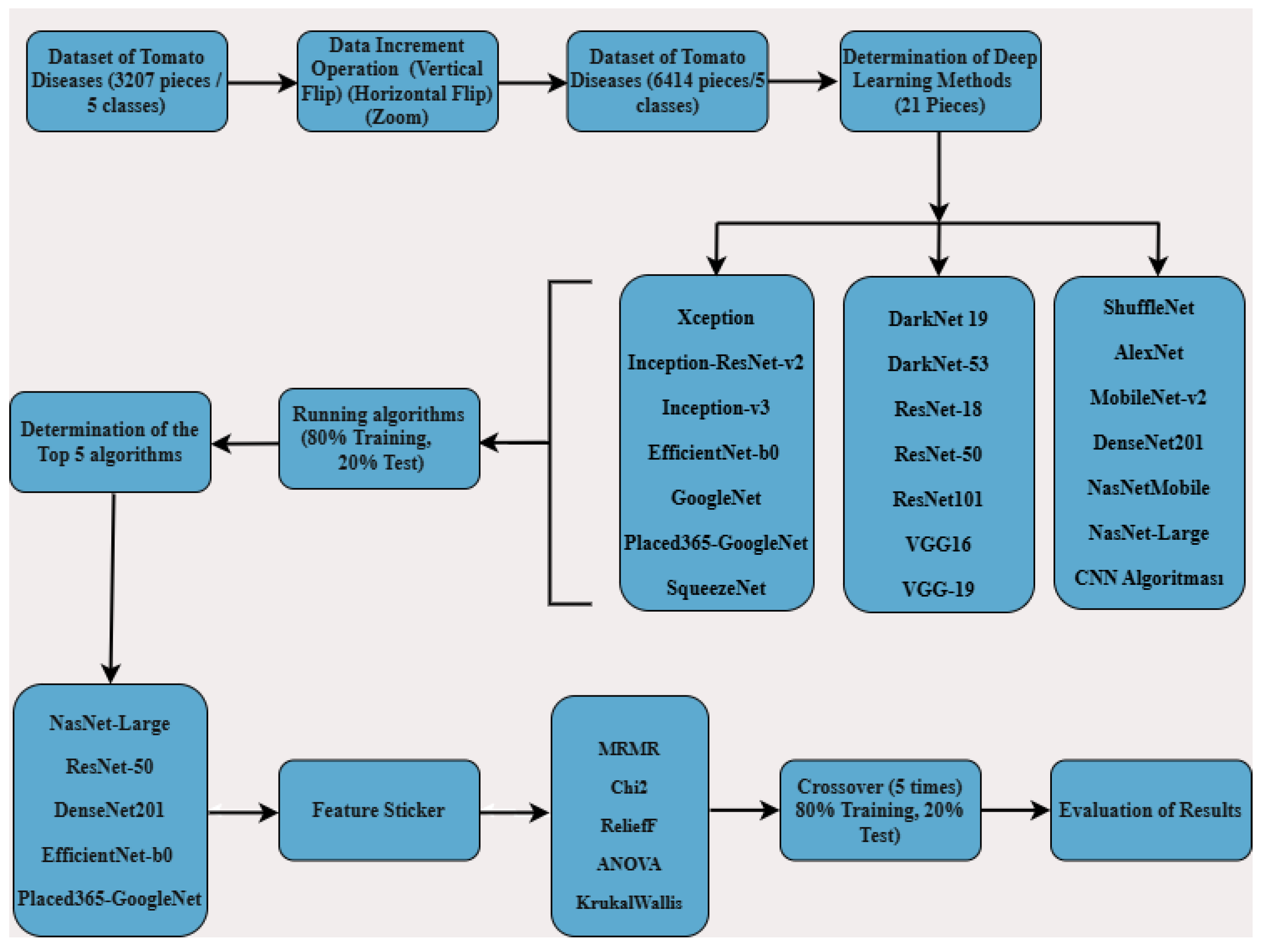
As shown in Figure 1 of the study, a five-class classification was carried out using original data of common tomato diseases—late blight, early blight, gray mold, bacterial canker—and healthy tomatoes. Initially, a total of 3,207 data samples were expanded to 6,414 using data augmentation techniques. These 6,414 data samples were then used to train models using 21 different deep learning algorithms, with 80% used for training and 20% for testing. From the results, the top 5 deep learning algorithms were identified. Feature extraction was applied using these 5 algorithms, resulting in the extraction of 1,000 features. Then, 100 features were selected using MRMR, Chi2, ReliefF, ANOVA, and Kruskal-Wallis methods. These selected features were split into 80% for training and 20% for testing, and reclassification was performed using machine learning algorithms with 5-fold cross-validation. The results obtained from this process were evaluated.

Figure 1. Tomato Disease Classification Block Diagram.

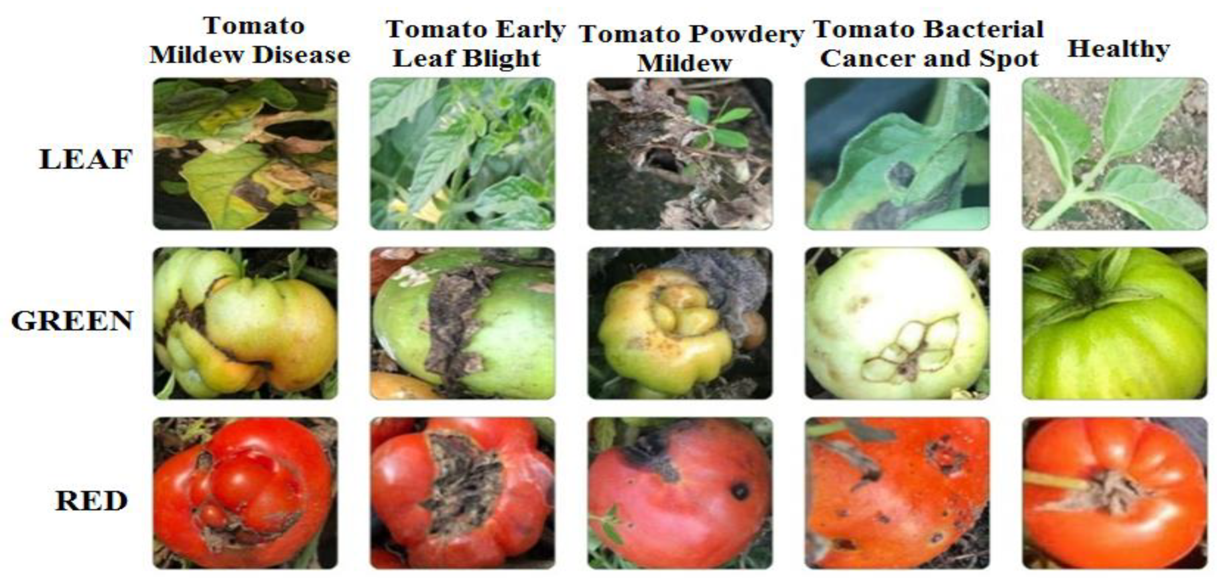
In this study, a dataset composed of unstructured images of red and green tomatoes and leaves, as shown in Figure 2, was used. This study aims to fill the gap in literature using this dataset and contribute to the development of more effective pest management strategies for agriculture.

Figure 2. Sample Images of Red and Green Tomatoes and Leaves.

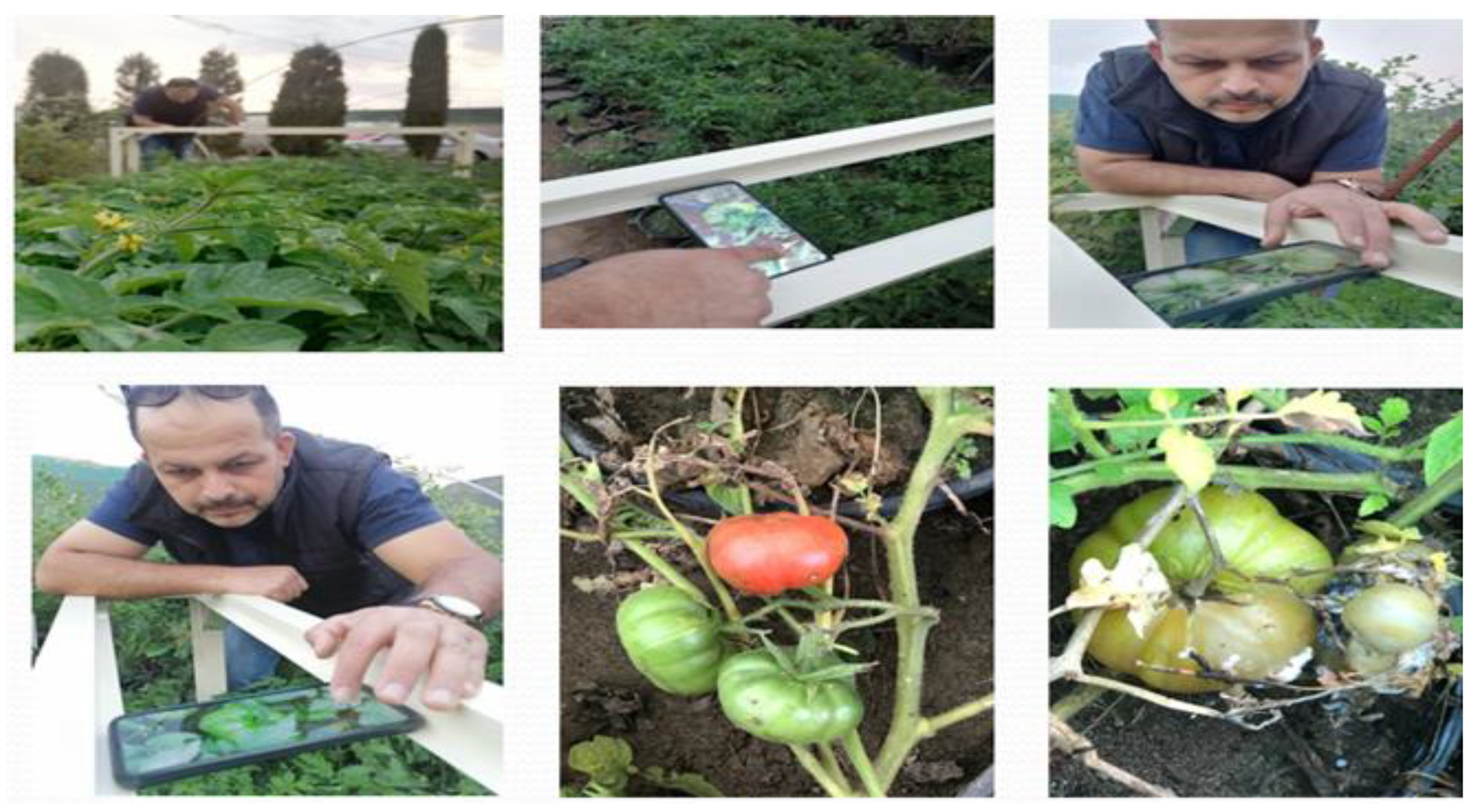
The tomato disease data were collected from the tomato greenhouse established in Kirkuk province, as shown in Figure 3. Tomato planting was carried out, and their development was monitored daily.

Figure 3. Images from the Greenhouse Where the Data Were Collected.

The images of the cultivated tomato plants were captured using the Redmi Note 9 Pro, which features an AI-powered quad-camera system. This system includes a 64-megapixel main camera with an f/1.89 aperture, an 8-megapixel ultra-wide-angle camera with an f/2.2 aperture, a 2-megapixel depth camera with an f/2.4 aperture, and a 5-megapixel macro camera also with an f/2.4 aperture and focal length.

As shown in Table 1, the dataset consists of 3,207 images of leaves affected by diseases such as late blight, early blight, gray mold, bacterial canker, and bacterial spot.

Table 1. Number of Original Data Samples.

Disease	Red	Leaf	Green	Total
Tomato Mildew Disease	374	369	122	865
Tomato Early Leaf Blight	110	277	97	484
Tomato Powdery Mildew	157	223	123	503
Tomato Bacterial Cancer and Spot	215	183	125	523
Normal Healthy Tomato	458	264	110	832
Total	1314	1316	577	3207

The data augmentation techniques used in this work are implemented through the ImageDataGenerator class of the TensorFlow Keras library. These techniques are designed to improve the ability of our model to recognize different image variations by increasing the diversity of our image-based data sets. The main data augmentation techniques used were rotation, shift, shear, zoom, flip, and brightness adjustment.

These parameters were used in the training process of the model and the ratios determined for each transformation technique were carefully selected to maximize the adaptability of the model to scenarios that the model may encounter on real world data. In terms of the number of data augmentations, approximately 2 to 4 augmented images were produced for each original image. This significantly increased the diversity of our dataset and allowed the model to learn from a wider range of data during training. As a result, these data augmentation techniques significantly improved the overall performance of our model and allowed it to work more effectively on complex image recognition tasks. As a result of the data augmentation method, as shown in Table 2, the study was carried out with a total of 6414 data, including Tomato Mildew Disease 1730, Tomato Early Leaf Blight 968, Tomato Canker Mildew 1006, Tomato Bacterial Cancer and Stain 1046 and Normal Healthy Tomato 1664.

Table 2. Augmented data counts.

Disease	Original Data				Augmented Data
Disease	Red	Leaf	Green	Total	Red	Leaf	Green	Total
Tomato Mildew Disease	374	369	122	865	748	738	244	1730
Tomato Early Leaf Blight	110	277	97	484	220	554	194	968
Tomato Powdery Mildew	157	223	123	503	314	446	246	1006
Tomato Bacterial Cancer and Spot	215	183	125	523	430	366	250	1046
Normal Healthy Tomato	458	264	110	832	916	528	220	1664
Total	1314	1316	577	3207	2628	2632	1154	6414

The computer used for training the deep learning algorithms is equipped with a 12th Gen Intel® Core™ i9-12900HX processor operating at 2.30 GHz, 32.0 GB of RAM, and a 64-bit operating system.

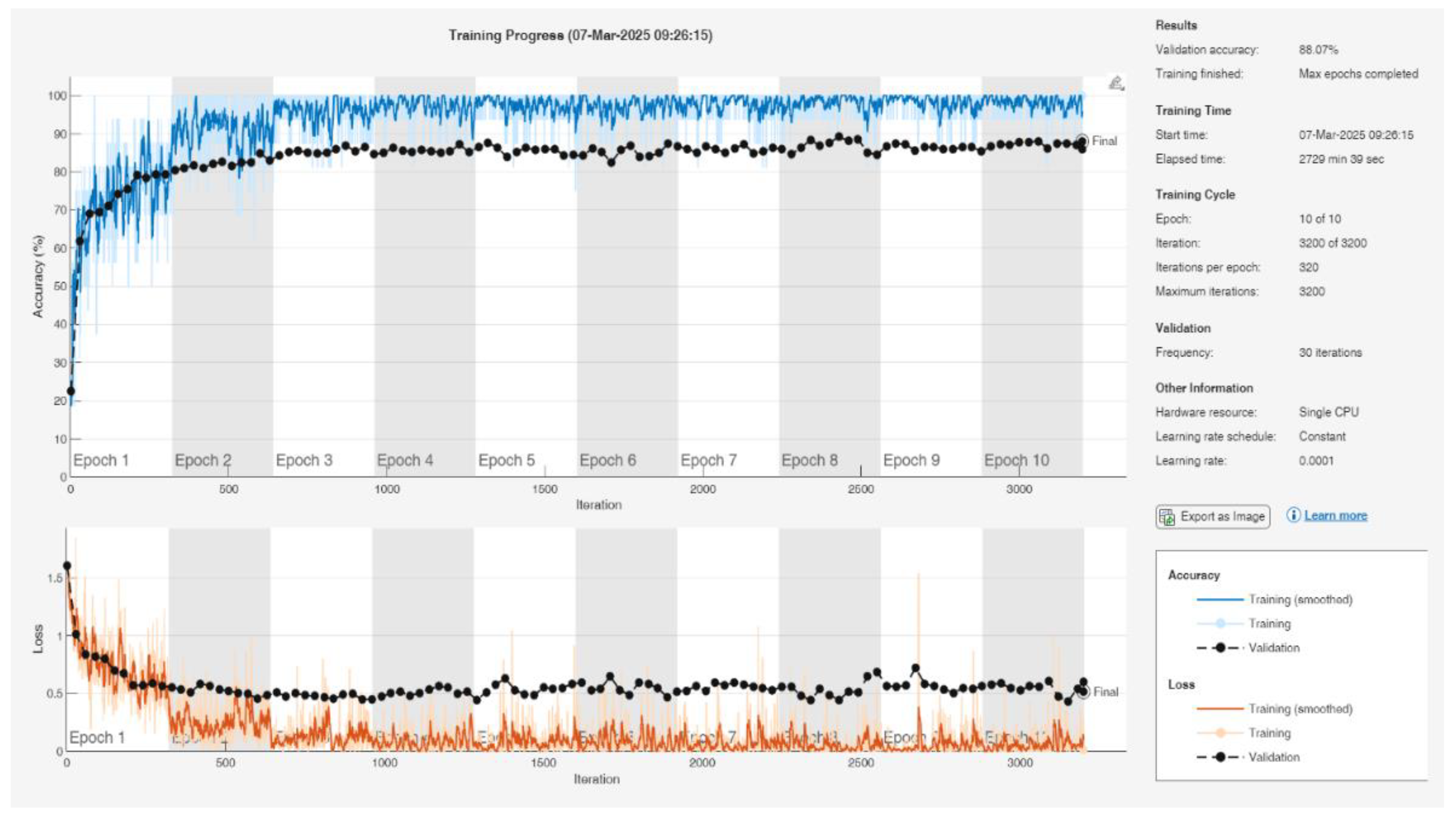
In the classification of tomato diseases, a total of 21 deep learning algorithms were employed, including CNN, Inception-ResNet-v2, GoogleNet, Places365-GoogleNet, SqueezeNet, DarkNet-53, ResNet-50, AlexNet, MobileNet-v2, EfficientNet-b0, DenseNet201, NasNetMobile, ResNet-18, DarkNet-19, VGG-19, ShuffleNet, Xception, Inception-v3, ResNet-101, VGG-16, and NasNet-Large. These models were trained using randomly selected data split into 80% for training and 20% for testing. The training parameters of the top five algorithms, those that achieved the highest classification accuracy, are presented in Table 3. MATLAB training result graphs and values of the NasNet-Large algorithm are given in Figure 4.

Table 3. Training parameters for the first 5 algorithms.

PARAMETER	NasNet-Large	ResNet-50	DenseNet-201	EfficientNet-b0	Placed365-GoogleNet
Initial Learning Rate	0.0001	0.00005	0.0001	0.0001	0.00005
Verification Frequency	30	30	30	30	30
Maximum Epoch Number	10	20	10	10	20
Mini-Batch Size	16	32	16	32	32
Mixing	Each epoch	Each epoch	Each epoch	Each epoch	Each epoch

Figure 4. Training Result Graphs and Performance Metrics of the NasNet-Large Algorithm in MATLAB.

3. Results

Tomato cultivation is one of the most developed agricultural sectors in Turkey. Due to the fact that tomatoes are a staple food widely consumed by the population, ensuring high productivity is of great importance. Therefore, this study aims to detect and classify four common diseases affecting tomato plants. The augmented dataset presented in Table 3.1 includes the training and testing accuracy rates, as well as the execution times for 21 different deep learning algorithms. Upon examining Table 4, it is observed that the NasNet-Large algorithm achieved the highest accuracy, with a training accuracy of 88.07% and a testing accuracy of 87.23%. However, this performance came at a significant computational cost, with a training time of 2729 minutes and 39 seconds, indicating a disproportionate time-to-performance ratio.

Considering both time and performance metrics, the ResNet-50 algorithm demonstrated a more balanced profile, achieving a training accuracy of 88.07% and a testing accuracy of 86.85%, with a training duration of 625 minutes and 25 seconds. This indicates that ResNet-50 offers a favorable trade-off between computational efficiency and classification performance.

Moreover, the EfficientNet-b0 algorithm yielded 86.53% training accuracy and 85.76% testing accuracy, while completing its training in just 140 minutes and 51 seconds. This highlights its rapid execution time combined with high classification accuracy, making it a promising candidate for time-sensitive applications.

Based on the evaluations and as illustrated in Figure 5 and Table 4, the CNN algorithm, with a training accuracy of 66.17% and a testing accuracy of 60.23%, and the DarkNet-19 algorithm, with a training accuracy of 62.67% and a testing accuracy of 57.16%, were identified as the two least effective models in terms of classification performance.

Table 4. Training and test accuracy rates and run times of deep learning algorithms.

No	Algorithms	Training Accuracy Rate	Test Accuracy Rate	Time
1	Nasecet-Large	88,07	87,23	2729min 39sec
2	Resecet-50	88,07	86,85	625 min 25sec
3	DenseNet-201	86,59	85,82	604min 50sec
4	EfficientNet-b0	86,53	85,76	140min 51sec
5	Placed365-GoogLeNet	86,36	85,76	273 min 55sec
6	Inception-v3	85,58	84,31	359min 54sec
7	Xception	84,8	83,15	733min 17sec
8	Nasecet-Mobile	84,18	82,53	214min 7sec
9	Resecet-101	84,1	82,18	1371min 33sec
10	Inception-Resecet-v2	84,02	80,94	594min 8sec
11	GoogleNet	82,93	82,17	140min 39sec
12	ShuffleNet	82,7	80,75	60min 2sec
13	DarkNet-53	80,75	77,6	566min 44sec
14	MobileNet-v2	79,58	77,14	319min 33sec
15	AlexNet	79,27	76,37	95min 34sec
16	SquuzeNet	77,71	74,31	110min 39sec
17	Resecet-18	77,63	74,34	187min 36sec
18	VGG-19	75,14	72,49	368min 19sec
19	VGG-16	68,28	69,60	382min 26sec
20	CNN	66,17	60,23	403 min 13sec
21	DarkNet-19	62,67	57,16	262min 26sec

Figure 5. Training and test accucary ratios of deep learning algorithms.

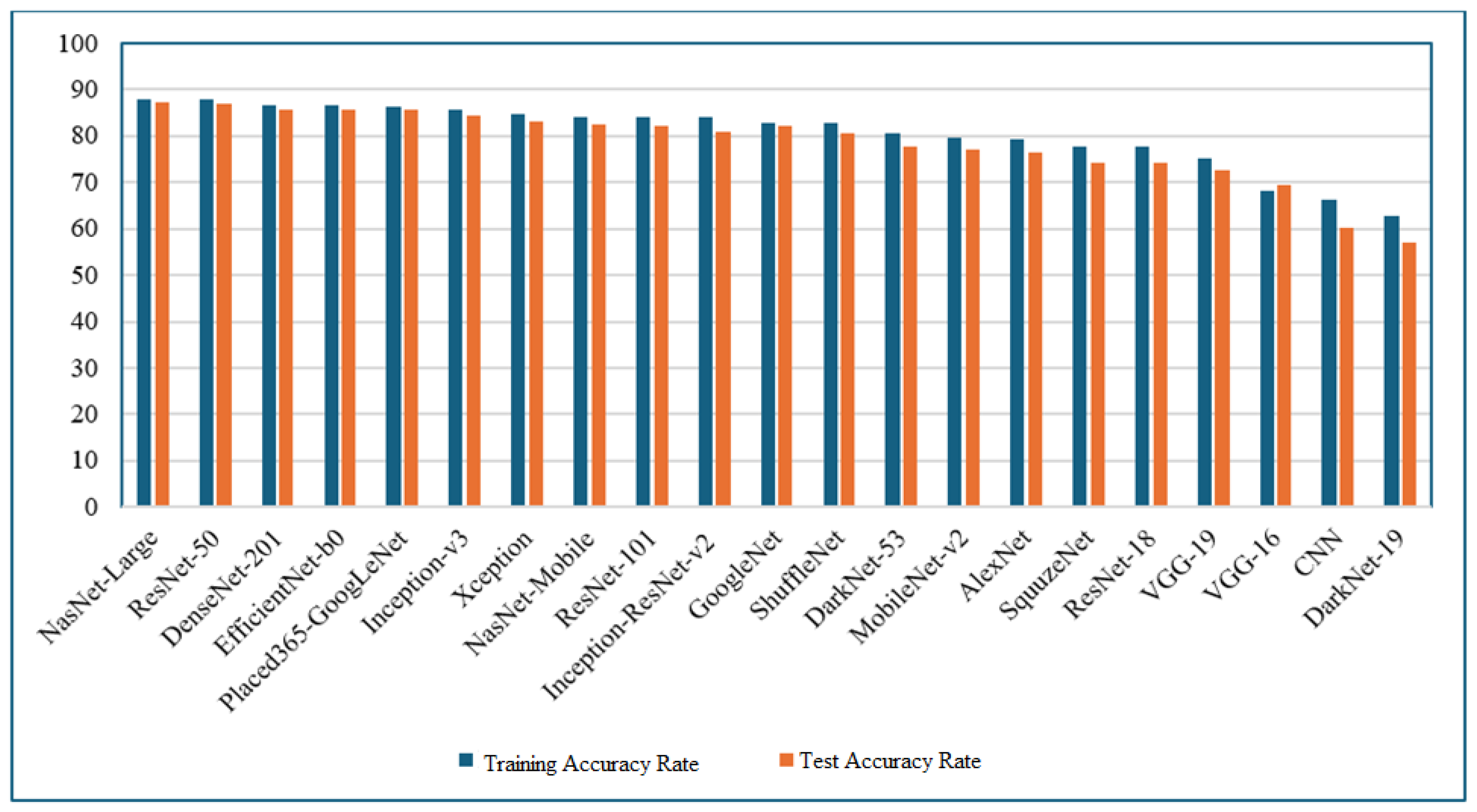
Figure 6 presents the confusion matrices and classification accuracy rates for the four most successful deep learning algorithms—NasNet-Large, ResNet-50, DenseNet201, and EfficientNet-b0—in the context of tomato disease classification. These matrices provide a comparative overview of each model’s ability to distinguish between disease classes and demonstrate their overall predictive effectiveness.

Figure 6. Disease classification accuracy rates of the top 4 deep learning methods using test comparison matrices (a) NasNet-Large (b) ResNet-50 (c) DenseNet201 (d) EfficientNet-b0.

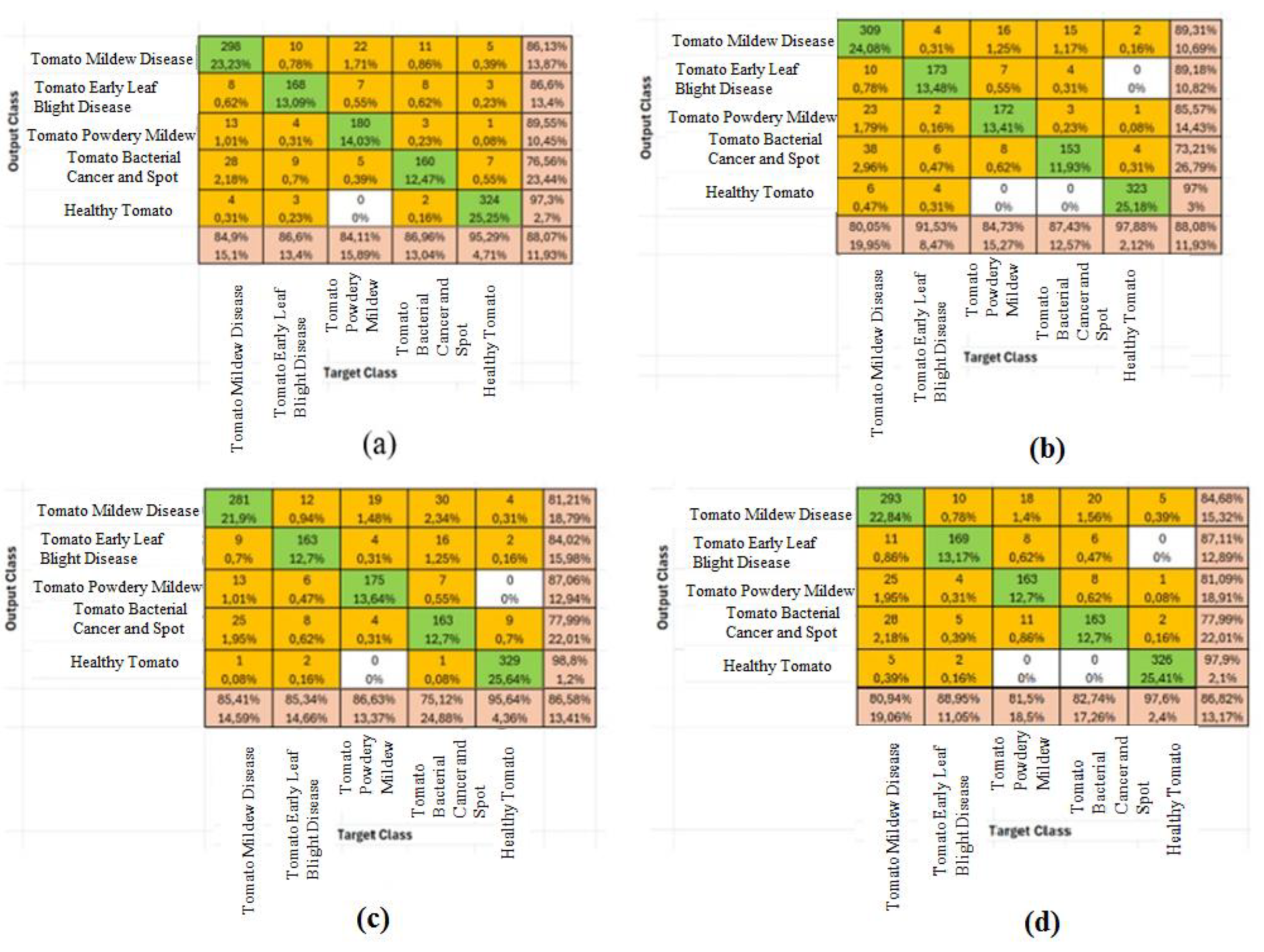
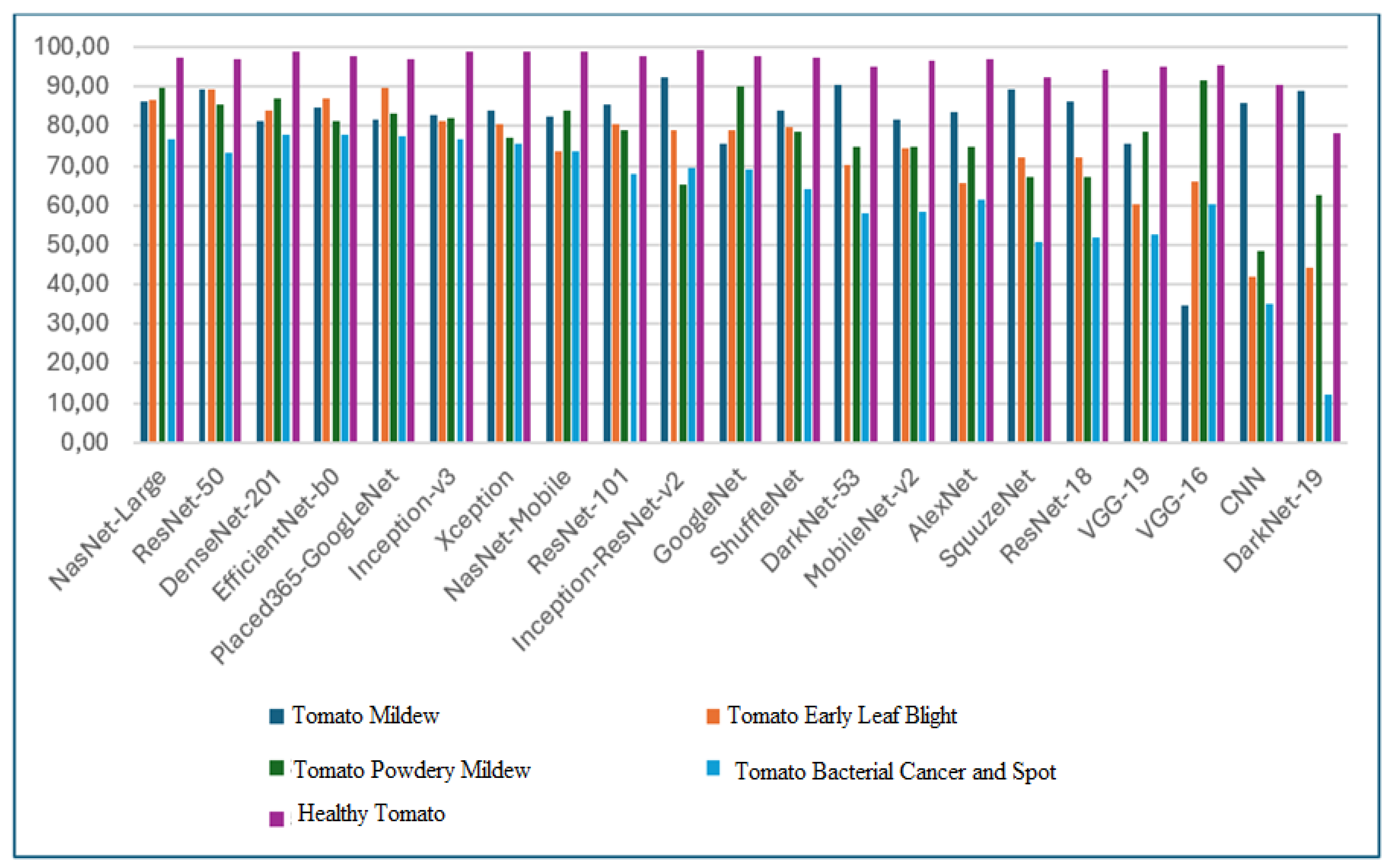
Table 5 shows the accuracy rates of 21 deep learning methods in disease classification using test comparison matrices.

As shown in Table 5, Late Blight Disease (Mildiyö) was classified with over 80% accuracy by 17 models, Early Blight by 8 models, Tomato Gray Mold by 9 models, and Healthy Tomato class by 20 models. In contrast, the Bacterial Canker and Spot Disease class was generally classified with relatively lower accuracy across most models. Late Blight achieved the highest classification accuracy of 92.2% using the Inception-ResNet-v2 algorithm, while the lowest accuracy of 34.68% was observed with VGG-16. Early Blight was best classified with accuracies ranging between 87% and 89% by Place365-GoogLeNet, ResNet-50, and EfficientNet-b0, whereas CNN and DarkNet-19 performed poorly, with accuracies of 41.75% and 44.33%, respectively. Tomato Gray Mold was best classified by the VGG-16 model, with accuracy values of 91.54% and 90.05%. Bacterial Canker and Spot Disease reached its highest accuracies with VGG-16 and VGG-19, at 91.54% and 78.61%, respectively; however, for most models, the accuracy in this class remained below 60%. For the Healthy Tomato class, very high accuracy levels exceeding 98% were achieved by Inception-ResNet-v2, DenseNet-201, Xception, and NasNet-Mobile.

Table 5. Accuracy rates of deep learning methods for disease classification with test data.

No	Algorithms	Mildew Disease	Early Leaf Blight	Powdery Mildew	Tomato Bacterial Cancer and Spot	Normal Healthy Tomato	Test Data Accuracy Rate
1	NasNet-Large	86,13	86,60	89,55	76,56	97,30	87,23
2	ResNet-50	89,31	89,18	85,57	73,21	97,00	86,85
3	DenseNet-201	81,21	84,02	87,06	77,99	98,80	85,82
4	EfficientNet-b0	84,68	87,11	81,09	77,99	97,90	85,76
5	Placed365-GoogLeNet	81,5	89,69	83,08	77,51	97	85,76
6	Inception-v3	82,66	81,44	82,09	76,56	98,80	84,31
7	Xception	83,82	80,41	77,11	75,60	98,80	83,15
8	NasNet-Mobile	82,37	73,71	84,08	73,68	98,80	82,53
9	ResNet-101	85,55	80,41	79,10	67,94	97,90	82,18
10	Inception-ResNet-v2	92,2	78,87	65,17	69,38	99,1	80,94
11	GoogleNet	75,43	78,87	90,05	68,9	97,6	82,17
12	ShuffleNet	83,82	79,90	78,61	64,11	97,30	80,75
13	DarkNet-53	90,46	70,10	74,63	57,89	94,89	77,6
14	MobileNet-v2	81,79	74,23	74,63	58,37	96,70	77,14
15	AlexNet	83,53	65,46	74,63	61,24	97,00	76,37
16	SquuzeNet	89,31	72,16	67,16	50,72	92,19	74,31
17	ResNet-18	86,42	72,16	67,16	51,67	94,29	74,34
18	VGG-19	75,72	60,31	78,61	52,63	95,20	72,49
19	VGG-16	34,68	65,98	91,54	60,29	95,50	69,60
20	CNN	85,84	41,75	48,26	34,93	90,39	60,23
21	DarkNet-19	88,73	44,33	62,69	11,96	78,08	57,16

The graphical representation of classification accuracy rates for each deep learning method is presented in Figure 7.

Figure 7. Disease classification accuracy rates of the deep learning method.

Based on the 5 most successful algorithms in terms of overall classification, Mildy mildew disease with ResNet-50 algorithm is 89.3%, leaf blight with ResNet-50 algorithm is 89.2% and Placed365-GoogLeNet algorithm is 89.7%, It is seen that NasNet-Large algorithm for Tomato Bacterial Mildew disease is the model with the highest classification rates with 89.5%, DenseNet-201 algorithm for Tomato Bacterial Cancer and Stain disease with 77.99% and DenseNet-201 algorithm for Healthy Tomato disease with 98.8% accuracy rates.

Considering the training and test success rates from Figure 6 and Figure 7, NasNet-Large, ResNet-50, DenseNet-201, EfficientNet-b0, Placed365-GoogLeNet algorithms are the 5 most successful deep learning methods.

Table 6. Performance comparison of classification results obtained by using 100 features obtained by feature selection methods.

Deep feature extraction methods	MRMR			Chi²			ReliefF
Deep feature extraction methods	Machine Learning Model	Training Accuracy Rate	Test Accuracy Rate	Machine Learning Model	Training Accuracy Rate	Test Accuracy Rate	Machine Learning Model	Training Accuracy Rate	Test Accuracy Rate
NasNet-Large	Fine KNN	83,53	86,70	Fine KNN	82,40	87,40	Fine KNN	84,30	86,60
	Fine Gaussian SVM	77,70	80,80	Cubic SVM	79,50	81,90	Cubic SVM	78,40	83,20
	Wide Neural Network	72,80	75,60	Wide Neural Network	73,10	75,80	Wide Neural Network	72,60	75,40
ResNet-50	KSubspace KNN	88,3	88,8	Subspace KNN	86,7	89,4	Subspace KNN	87,8	90,7
	Cubic SVM	83,4	84,4	Cubic SVM	82	83,7	Cubic SVM	83	86,2
	Wide Neural Network	77,8	79,3	Wide Neural Network	77,6	78,6	Wide Neural Network	76,8	79,1
DenseNet-201	Subspace KNN	86,6	90,8	Subspace KNN	86,3	90,4	Subspace KNN	87,5	90,2
	Cubic SVM	82,6	84,,6	Cubic SVM	81,9	86,2	Cubic SVM	82,9	84,9
	Wide Neural Network	76	78,9	Wide Neural Network	76	78,4	Wide Neural Network	77	79,8
EfficientNet-b0	Subspace KNN	89,3	91,7	Fine KNN	88,4	92	Subspace KNN	89,6	91,2
	Cubic SVM	84,7	85,4	Cubic SVM	83,6	86,6	Cubic SVM	85,4	87,1
	Wide Neural Network	79,3	77,7	Wide Neural Network	78	79,4	Wide Neural Network	78,9	81
Placed365-GoogLeNet	Subspace KNN	84,4	86,7	Fine KNN	82,8	85,4	Subspace KNN	85,6	87,9
	Cubic SVM	79,4	83,1	Cubic SVM	79,6	82,4	Cubic SVM	80,5	81,2
	Wide Neural Network	73,3	75	Wide Neural Network	73,8	76,2	Wide Neural Network	73,7	74,4

When the results obtained in Table 4 are evaluated and the heat map in Figure 8 is created, it is seen that the 5 deep learning algorithms with the highest test accuracy are NasNet-Large, ResNet-50, DenseNet-201, EfficientNet-b0 and Placed365-GoogLeNet models. Using the algorithms with the best results, 1000 features were extracted with the feature extraction process. After feature extraction, the number of features was reduced to 100 by using MRMR, Chi2, ReliefF, ANOVA and KrukalWallis methods to select the most successful features in classification. Since the success rates of the classification processes using the datasets obtained with ANOVA and KrukalWallis feature extraction methods remained at low values compared to other methods, the results of these two feature selection algorithms were not shared. This new data set was divided into 80% Training and 20% Test, and reclassification was performed with machine learning algorithms by applying 5-fold cross-validation method. Table 5 shows the results of the 3 machine learning algorithms that produced the best classification results using 100 features.

Figure 8. Heat map of the 5 deep learning algorithms with the highest test accuracy.

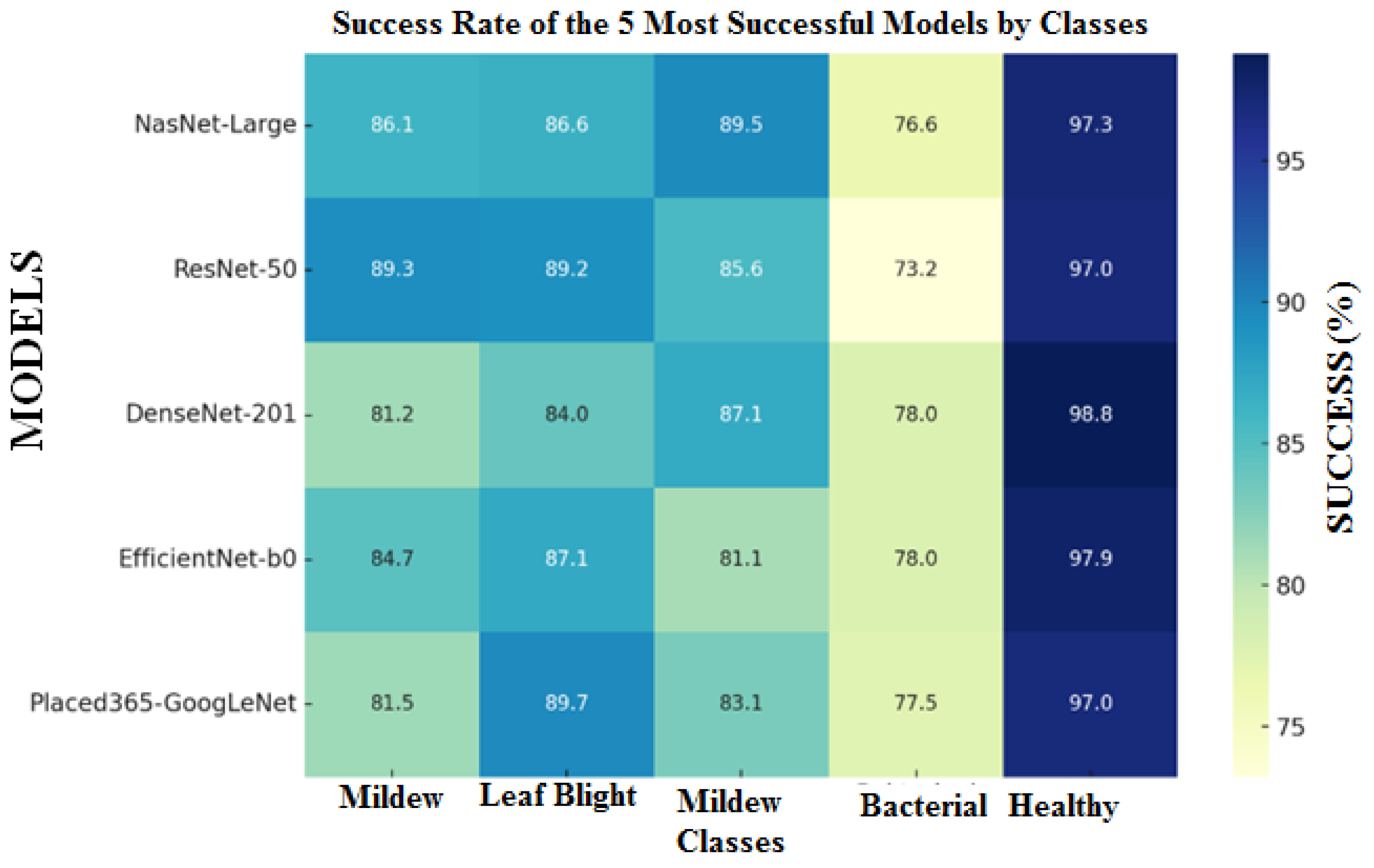
Table 7. Training and test accuracy results obtained with 100 features.

Deep feature extraction methods	Machine Learning Model	MRMR Training Accuracy Rate	Test Accuracy Rate	Machine Learning Model	Chi2 Training Accuracy Rate	Test Accuracy Rate	Machine Learning Model	ReliefF Training Accuracy Rate	Test Accuracy Rate
NasNet-Large	Fine KNN	83,53	86,70	Fine KNN	82,40	87,40	Fine KNN	84,30	86,60
ResNet-50	KSubspace KNN	88,3	88,8	Subspace KNN	86,7	89,4	Subspace KNN	87,8	90,7
DenseNet-201	Subspace KNN	86,6	90,8	Subspace KNN	86,3	90,4	Subspace KNN	87,5	90,2
EfficientNet-b0	Subspace KNN	89,3	91,7	Fine KNN	88,4	92	Subspace KNN	89,6	91,2
Placed365-GoogLeNet	Subspace KNN	84,4	86,7	Fine KNN	82,8	85,4	Subspace KNN	85,6	87,9
Ortalama		86,43	88,94		85,32	88,92		86,96	89,32
Standart Sapma		2,20	2,06		2,33	2,31		1,84	1,77
Varyans Analiz		4.86	4.23		5.45	5.32		3.38	3.13

When Table 6 is examined, it is seen that the Subspace KNN classifier provides the highest test accuracies in almost all data sets with 100 features, the Cubic SVM classifier is generally good but does not reach as high results as the Subspace KNN classifier, and the Wide Neural Network classifier generally gives the lowest test accuracies. It is also seen that the Subspace KNN classifier generally provides the highest test accuracy rates in the DenseNet-201 and ResNet-50 deep learning algorithms.

Table 7 compares training and test accuracy rates based on 100 features selected from a set of 1000 deep features using various feature selection methods, including MRMR, Chi2, and ReliefF, applied to different deep feature extraction techniques. According to this table, the highest test accuracy of 92% was achieved when features extracted from the EfficientNet-b0 model were selected using the Chi2 method and classified using the Fine K-Nearest Neighbors (Fine KNN) machine learning algorithm.

To determine the most consistent classification performance, the mean, standard deviation, and variance of the obtained results were calculated. Based on these calculations, the ReliefF method demonstrated the most stable performance, with an average test accuracy of 89.32%.

Among the deep feature extraction models examined, features derived from EfficientNet-b0 consistently yielded the highest accuracy rates across all feature selection methods. Features extracted from DenseNet-201 and ResNet-50 also showed strong classification performance with high accuracy values. In contrast, features derived from the NasNet-Large model resulted in relatively lower classification accuracy, around 86%, compared to other models.

When considering standard deviation and variance analyses, the ReliefF method exhibited lower standard deviation values in both training and test accuracies, indicating more stable performance. In contrast, the Chi² method showed greater variability in accuracy rates.

As a result, it can be said that the combination that produces the most stable results in the classifications using 100 features is the classification of the features extracted from the EfficientNet-b0 model with machine learning algorithms by selecting them with the ReliefF method.

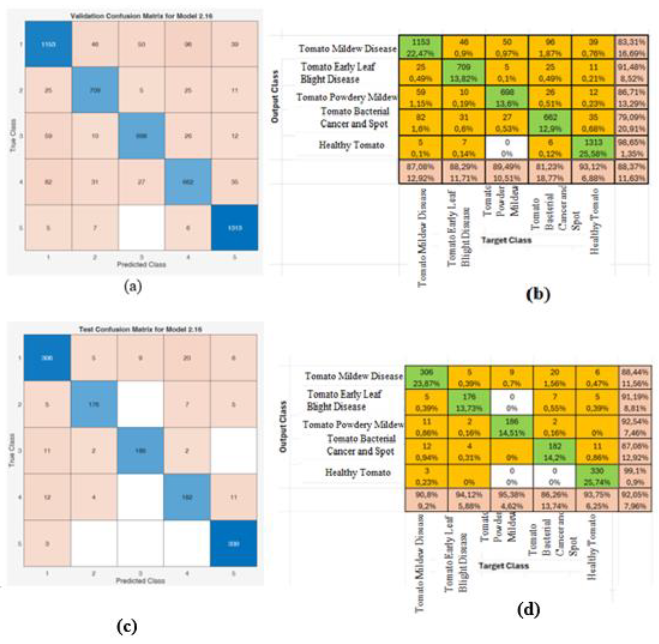
Since the best result was obtained using the EfficientNet-b0 algorithm, the training and test confusion matrices based on the Chi2 feature selection method applied to this algorithm are presented in Figure 9. As seen in Figure 9, when the number of features was reduced using the Chi2 method with the EfficientNet-b0 algorithm, a training accuracy of 88.4% and a test accuracy of 92% were achieved.

Figure 9. EfficientNet-b0 algorithm Chi2 method training and test comparison matrices (a) Training comparison matrix (b) Disease classification accuracy rates using training comparison matrices (c) Test comparison matrix (d) Disease classification accuracy rates using test comparison matrices.

In this study, a five-class classification was performed, covering the most common tomato diseases—late blight, early blight, gray mold, bacterial cancer, and healthy tomatoes. The dataset used in the study is entirely original, consisting of 6,414 images collected from three groups: leaves, red tomatoes, and green tomatoes, captured in the production field. These data were processed using 21 deep learning algorithms, and their results were evaluated. Among these, the best-performing models were identified as NasNet-Large, ResNet-50, DenseNet201, EfficientNet-b0, and Placed365-GoogLeNet.

From each of the selected models, 1,000 features were extracted. Feature selection algorithms (MRMR, Chi2, ReliefF, ANOVA, and Kruskal-Wallis) were then applied to select 100 features from each set. The newly constructed datasets were split into 80% training and 20% test sets, and models were trained using 5-fold cross-validation with various machine learning algorithms. As a result, a total of 51 combinations were evaluated, comprising 21 deep learning algorithms and 5 feature selection methods.

Among these combinations, the highest performance was achieved with the EfficientNet-b0 algorithm, where the Chi2 feature selection method yielded a training accuracy of 88.4% and a test accuracy of 92%. Furthermore, it can be concluded that the most stable results in classifications using 100 features were obtained when features extracted from EfficientNet-b0 were selected using the ReliefF method and classified with machine learning algorithms.

In conclusion, this study demonstrates the potential and applicability of deep learning-based disease diagnosis systems in the agricultural sector. More effective integration of technology in agricultural practices can enhance both production processes and product quality, thus contributing to the widespread adoption of sustainable agricultural practices. In this context, the study can be considered an important step that may inspire future research.

4. Discussion

The tomato plant is one of the most widely cultivated agricultural products globally, and various diseases affecting its leaves, stems, or fruits can significantly reduce yield. Early detection of these diseases is of critical importance, not only to prevent economic losses but also to enable the implementation of environmentally sustainable pest management strategies. Artificial intelligence-based approaches, particularly those utilizing deep learning-supported image processing techniques, have demonstrated high success in this regard.

In this study, a performance analysis of classification models was conducted by combining deep features extracted from 21 deep learning architectures—including NasNet-Large, ResNet-50, and DenseNet-201—with five different feature selection methods: MRMR, Chi2, ReliefF, ANOVA, and Kruskal-Wallis.

Table 8 presents a summary of previous studies related to the classification of tomato diseases, including the methods employed and the reported accuracy rates.

Table 8. Similar studies on tomato diseases.

Reference	Method	Accuracy Rate
Bakr, Abdel-Gaber et al. 2022 [25]	DenseNet201, Transfer Learning	Training: %99.84, Verification : %99.30
Zayani, Ammar et al. 2024 [26]	YOLOv8	%66.67
Abbas, Jain et al. 2021 [27]	C-GAN + DenseNet121	5 Classes: %99.51, 7 Classes: %98.65, 10 Classes: %97.11
Trivedi, Gautam et al. 2021 [28]	Recommended Deep Neural Network	%98.49
Khasawneh, Faouri et al. 2022 [29]	DenseNet201, Darknet-53	%99.2
Albahli and Nawaz 2022 [30]	DenseNet-77 + CornerNet	%98.4
Ahmed, Hasan et al. 2022 [31]	MobileNetV2 + Special Classifier	%99.30
Kabir Oni and Tanzin Prama 2025 [32]	Special CNN	%95.2
This study	EfficientNet-b0 + Chi2 + Fine KNN	%92

Unlike the academic studies and other studies in Table 8, the studies carried out so far have been based on only leaf, only tomato data and limited images. In this study, red tomato, green tomato and leaf data taken in the natural environment were used. In the previous studies, deep learning methods were used and the algorithms with the best results were determined. In this study, the NasNet-LArge algorithm gave the best results without feature extraction, but it was observed that the accuracy rates of the EfficientNet-b0 algorithm were higher after feature extraction. In this study, 21 deep learning algorithms, the feature extraction of the first 5 algorithms among these algorithms, the application of five different feature selection methods to these algorithms, and even the classification process using machine learning methods (KNN, SVM and ANN) within each feature. Therefore, the originality of this study in the current situation and the comparisons made will guide the studies to be carried out not only for tomato diseases but also for the classification of different types of diseases.

Author Contributions

Conceptualization, H.T. and A.G.; methodology, H.T. and A.G. ; soft-ware, H.T ; validation, H.T. and A.M.A.S. ; formal analysis, A.M.A.S. and M.Y.A.B. ; investigation, A.M.A.S. ; resources, H.T. and A.M.A.S. ; data curation, A.M.A.S. and M.Y.A.B. ; writing—original draft preparation, H.T.. ; writing—review and editing, A.G.. and H.T. ; visualization, H.T and A.M.A.S.; supervision, H.T., A.G. and A.M.A.S; project administration, A.G. and H.T.; funding acquisition, A.M.A.S. . All authors have read and agreed to the published version of the manuscript.

Data Availability Statement

The data presented in this study are not publicly available due to privacy and confidentiality restrictions. However, specific details regarding the dataset and ex-perimental methodology have been provided in the manuscript to ensure transparency and re-producibility. Researchers who require further information may contact the corresponding au-thor, subject to compliance with applicable ethical, institutional, and legal constraints.

Acknowledgments

This study was produced from Adnan Mohammad Anwer Shakarji unpublished Ph.D. thesis.

Conflicts of Interest

The authors declare no conflicts of interest.

References

Takale, D.G. , et al. Image Processing and Machine Learning for Plant Disease Detection. in International Conference on Artificial-Business Analytics, Quantum and Machine Learning, 2023. Springer.
Ferentinos, K.P. , Deep learning models for plant disease detection and diagnosis. Computers and electronics in agriculture, 2018. 145: p. 311-318. [CrossRef]
Too, E.C. , et al., A comparative study of fine-tuning deep learning models for plant disease identification. Computers and Electronics in Agriculture, 2019. 161: p. 272-279. [CrossRef]
Demirci, D. , et al., DOMATES HASTALIĞI TAHMINI IÇIN GERÇEK ZAMANLI UYGULAMA. Eskişehir Osmangazi Üniversitesi Mühendislik ve Mimarlık Fakültesi Dergisi, 2022. 30(1): p. 90-95.
Rubanga, D.P. , et al., A deep learning approach for determining effects of Tuta Absoluta in tomato plants. arXiv:2004.04023, 2020.
Roy, A.M. and J. Bhaduri, A deep learning enabled multi-class plant disease detection model based on computer vision. Ai, 2021. 2(3): p. 413-428. [CrossRef]
Khan, A. , et al. Early and accurate detection of tomato leaf diseases using tomformer. in 2023 21st International Conference on Advanced Robotics (ICAR), 2023. IEEE.
Wagle, S.A. , A Deep Learning-Based Approach in Classification and Validation of Tomato Leaf Disease. Traitement du signal, 2021. 38(3). [CrossRef]
Kılıçarslan, S. and I. Pacal, Domates Yapraklarında Hastalık Tespiti İçin Transfer Öğrenme Metotlarının Kullanılması. Mühendislik Bilimleri ve Araştırmaları Dergisi, 2023. 5(2): p. 215-222.
Kotwal, J.G., R. Kashyap, and P.M. Shafi, Artificial driving based EfficientNet for automatic plant leaf disease classification. Multimedia Tools and Applications, 2024. 83(13): p. 38209-38240. [CrossRef]
Baki, D. , Domates (Solanum lycopersicum L.) bakteriyel öz nekrozu hastalık etmenleri Dickeya chrysanthemi, Pectobacterium carotovorum subsp. carotovorum, Pseudomonas cichorii, Pseudomonas corrugata, Pseudomonas fluorescens, Pseudomonas mediterranea ve Pseudomonas viridiflava’nın LNA probe kullanılarak real-time PCR tanısı ve hastalıklı bitki dokularından tespiti. 2014.
Fidan, H. and N. Sarı, Domateste Tomato spotted wilt virüs’ üne karşı dayanıklılığı kıran izolatının fenotipik karakterizasyonu. Mediterranean Agricultural Sciences, 2019. 32(3): p. 307-314.
Mutlu, G. and T. Üstüner, Elazığ ili domates alanlarında fungal hastalıkların yaygınlığı ve şiddetinin saptanması. Türk Tarım ve Doğa Bilimleri Dergisi, 2017. 4(4): p. 416-425.
Çaplık, D. , et al., Elazığ ili domates ve biber alanlarında fitoplazma hastalıklarının tespiti ve karakterizasyonu. Mustafa Kemal Üniversitesi Tarım Bilimleri Dergisi, 2022. 28(2): p. 269-278.
Albayrak, Ü., A. Gölcük, and S. Aktaş, Agaricus bisporus’ ta görüntü tabanlı hastalık sınıflandırması için kapsamlı veri seti. Mantar Dergisi, 2024. 15(1): p. 29-42.
Yasar, A., A. Golcuk, and O.F. Sari, Classification of bread wheat varieties with a combination of deep learning approach. European Food Research and Technology, 2024. 250(1): p. 181-189. [CrossRef]
Golcuk, A. and A. Yasar, Classification of bread wheat genotypes by machine learning algorithms. Journal of Food Composition and Analysis, 2023. 119: p. 105253. [CrossRef]
Chaerani, R. and R.E. Voorrips, Tomato early blight (Alternaria solani): the pathogen, genetics, and breeding for resistance. Journal of general plant pathology, 2006. 72: p. 335-347. [CrossRef]
Shakarji, A. and A. Gölcük, Classification of Tomato Diseases Using Deep Learning Method. Journal of Intelligent Systems & Internet of Things, 2025. 14(2). [CrossRef]
Soylu, E.M., Ş. Kurt, and S. Soylu, In vitro and in vivo antifungal activities of the essential oils of various plants against tomato grey mould disease agent Botrytis cinerea. International journal of food microbiology, 2010. 143(3): p. 183-189. [CrossRef]
Nowicki, M. , et al., Potato and tomato late blight caused by Phytophthora infestans: an overview of pathology and resistance breeding. Plant disease, 2012. 96(1): p. 4-17. [CrossRef]
Çelik, İ. , et al., Domates lekeli solgunluk virüsü (TSWV)’ne dayanıklı sivri biber hatlarının geliştirilmesi. Derim, 2018. 35(1): p. 27-36.
Felipe, V. , et al., Xanthomonas vesicatoria virulence factors involved in early stages of bacterial spot development in tomato. Plant Pathology, 2018. 67(9): p. 1936-1943. [CrossRef]
Horuz, S., Ş. T. Karut, and Y. Aysan, Domates bakteriyel kanser ve solgunluk hastalığı etmeni Clavibacter michiganensis subsp. michiganensis’ in tohumda aranması ve tohum uygulamalarının patojen gelişimine etkisinin belirlenmesi. Tekirdağ Ziraat Fakültesi Dergisi, 2019. 16(3): p. 284-296.
Bakr, M. , et al., Tomato disease detection model based on densenet and transfer learning. Applied Computer Science, 2022. 18(2): p. 56-70. [CrossRef]
Zayani, H.M. , et al., Deep learning for tomato disease detection with yolov8. Engineering, Technology & Applied Science Research, 2024. 14(2): p. 13584-13591. [CrossRef]
Abbas, A. , et al., Tomato plant disease detection using transfer learning with C-GAN synthetic images. Computers and electronics in agriculture, 2021. 187: p. 106279. [CrossRef]
Trivedi, N.K. , et al., Early detection and classification of tomato leaf disease using high-performance deep neural network. Sensors, 2021. 21(23): p. 7987. [CrossRef]
Khasawneh, N., E. Faouri, and M. Fraiwan, Automatic detection of tomato diseases using deep transfer learning. Applied Sciences, 2022. 12(17): p. 8467. [CrossRef]
Albahli, S. and M. Nawaz, DCNet: DenseNet-77-based CornerNet model for the tomato plant leaf disease detection and classification. Frontiers in plant science, 2022. 13: p. 957961. [CrossRef]
Ahmed, S. , et al., Less is more: Lighter and faster deep neural architecture for tomato leaf disease classification. IEEE Access, 2022. 10: p. 68868-68884. [CrossRef]
Kabir Oni, M. and T. Tanzin Prama, Optimized Custom CNN for Real-Time Tomato Leaf Disease Detection. arXiv e-prints, 2025: p. arXiv:2502.18521.

Disclaimer/Publisher’s Note: The statements, opinions and data contained in all publications are solely those of the individual author(s) and contributor(s) and not of MDPI and/or the editor(s). MDPI and/or the editor(s) disclaim responsibility for any injury to people or property resulting from any ideas, methods, instructions or products referred to in the content.

© 2025 by the authors. Licensee MDPI, Basel, Switzerland. This article is an open access article distributed under the terms and conditions of the Creative Commons Attribution (CC BY) license (http://creativecommons.org/licenses/by/4.0/).

Copyright: This open access article is published under a Creative Commons CC BY 4.0 license, which permit the free download, distribution, and reuse, provided that the author and preprint are cited in any reuse.