
Submitted:
13 May 2025
Posted:
15 May 2025
You are already at the latest version
Abstract
The 3DGS technology is a hot research direction in the current fields of computer vision and robotic perception. The initialization process of the 3DGS system requires obtaining the initial point cloud of the scene and the camera pose to assist in the establishment of the Gaussian map. Most of the research on initialization methods adopt the COLMAP system, which makes the overall time for establishing the Gaussian map relatively long. Based on this, in this study, the ORB-SLAM initialization method is first adopted to obtain the initial point cloud and the camera pose, which shortens the initialization time by 10 times. Secondly, in order to improve the reconstruction quality of the 3DGS, we introduce the LGSBA algorithm during the 3DGS training process. At the same time, our system uses ROS to achieve a tight coupling between the ORB-SLAM and the 3DGS system. On the basis of not affecting the reconstruction quality of the 3DGS, we finally achieve a significant superiority over the system that combines COLMAP and the traditional 3DGS in terms of both optimization time and optimization quality.
Keywords:
3D reconstruction
; SLAM
; 3D Gaussian splatting
; bundle adjustment
1. Introduction
Recently, 3DGS [1] has emerged as a cutting-edge method for generating dense and efficient maps from sparse 3D points. Unlike traditional 3D reconstruction techniques which center around accuracy and system integrity, 3DGS is dedicated to refine and densify sparse maps, offering a more efficient and flexible approach to creating high-quality scene representations, which makes it particularly valuable for real-time applications.
A critical challenge in 3DGS lies in its initialization process, which heavily depends on the quality of initial camera poses and point clouds. These inputs are typically provided by SfM methods such as COLMAP [2], which rely on extensive Bundle Adjustment optimization to refine camera poses. However, traditional BA focuses solely on maximizing pose accuracy without explicitly accounting for the quality of the reconstructed map. Consequently, while BA-refined poses are geometrically precise, they do not necessarily yield optimal Gaussian maps when integrated into a 3DGS system. This concern is not only pertinent to 3DGS-based SLAM but also to the broader realm of 3DGS optimization. Therefore, achieving a balance between pose precision and map reconstruction quality represents a critical and valuable research direction for enhancing both the fidelity of the reconstruction and the visual quality of rendered images.
In this article, we introduce an extension to the conventional BA optimization process, termed LGSBA, which is designed to enhance the quality of the Gaussian map produced by 3DGS. Specifically, our approach first employs traditional BA to obtain relatively accurate camera poses. Subsequently, LGSBA refines these poses using a sliding window that associates adjacent keyframes, and incorporates a loss function that evaluates the rendering quality of the Gaussian map. This additional optimization stage effectively balances the need for pose accuracy with the objective of high-quality map reconstruction.
Furthermore, we propose a tightly coupled online reconstruction framework based on ORB-SLAM, integrated with the Robot Operating System for real-time communication. In our system, ORB-SLAM is employed to pre-select keyframes and provide initial camera poses and point clouds in real time, thereby eliminating the initialization bottleneck in the 3DGS reconstruction process. The combination of our LGSBA optimization and the online ORB-SLAM framework consistently produces Gaussian maps that surpass those obtained via both traditional 3DGS optimization and the improved Scaffold-GS method, as evidenced by superior rendering quality metrics. This integrated approach not only accelerates the overall process but also yields high-quality 3DGS maps, demonstrating its effectiveness in both offline and real-time applications.
The key contributions of this article are summarized as follows:
- Worse Pose but Better 3DGS: Our findings reveal that the quality of initial camera poses and point cloud information significantly influences the subsequent 3DGS optimization process. Remarkably, our experiments demonstrate for the first time that higher precision in these initial inputs does not necessarily lead to better Gaussian maps. In some cases, particularly in outdoor scenes, overly accurate poses that strictly conform to the physical world may paradoxically degrade the quality of the Gaussian map.
- ORB-based Initialization for 3DGS: We propose an ORB-based approach for initializing 3DGS that utilizes camera poses from keyframes and aggregates point clouds from all keyframes. This method not only enables real-time processing and supports large-scale image sequences, but also ensures that the Gaussian map is built upon high-quality initial inputs.
- Sliding Window for Local Gaussian Splatting Bundle Adjustment: We introduce a sliding window technique during the 3DGS training process to optimize the poses of viewpoints within a localized window centered on the current viewpoint. In this approach, the Gaussian map is first refined to enhance its local structure, followed by an optimization of all poses in the window by minimizing the discrepancy between rendered and captured images. This dynamic process substantially improves map quality and rendering fidelity.
- Tightly Coupled Online 3DGS Optimization: We further propose a tightly coupled 3DGS optimization system that integrates with ORB-SLAM’s various threads to acquire real-time updates of point clouds and camera poses. Leveraging ROS for seamless communication, this framework continuously refines the 3DGS map online. Our practical experiments demonstrate that this integrated approach not only accelerates the overall mapping process but also significantly enhances the quality of the final Gaussian maps.
- Open-Source Codebase: To support further research and development in this field, we release our code and experimental results at https://github.com/wla-98/worse-pose-but-better-3DGS.
2. Related Work
2.1. 3D Gaussian Splatting
Benefiting from its explicit representation, short training time, and real-time rendering speed, 3DGS [1] has quickly outpaced Neural Radiance Fields [3] to become a prominent research focus in the field of 3D reconstruction. Numerous studies aim to enhance the pixel-level scene quality generated by 3DGS, which remains a key objective of 3DGS optimization.
Some studies [4,5] focus on optimizing the original parameters of 3DGS. However, parameter adjustments often require extensive experimentation and are closely tied to the specific characteristics of a given scene, limiting their generalizability. Other studies [6,7,8] improve rendering quality by incorporating depth estimation information, but acquiring depth data involves additional resource costs.
Despite these advancements, limited research has specifically explored how the initialization of camera poses and sparse point clouds impacts subsequent 3DGS results. Furthermore, most 3DGS reconstruction rely on COLMAP [2] pipeline, which consumes substantial computational resources when processing large image sets, significantly reducing the efficiency of scene reconstruction. Addressing this limitation is a key objective of this article.
2.2. Visual SLAM
Direct SLAM methods [9,10,11,12] excel in handling low-texture and dynamic environments. However, due to their assumption of consistent grayscale intensity, these methods are highly sensitive to illumination changes and noise, which makes them less suitable for real-world applications. Feature-based SLAM [13,14,15,16,17,18] is highly robust, delivering excellent real-time performance and supporting multi-task parallel processing to construct high-precision maps. These systems integrate seamlessly with data from other sensors, providing accurate and reliable solutions for localization and mapping. However, they produce sparse point cloud maps, which hinder downstream tasks and demand considerable time for parameter tuning.
NeRF-based SLAM [3,19,20,21,22,23,24] excels in 3D dense modeling, rendering novel viewpoints, and predicting unknown regions, significantly enhancing 3D model generation and processing under optimal observational inputs. Nevertheless, these methods depend on large amounts of data and computational resources for neural network training, making real-time performance difficult to achieve. Furthermore, their implicit representations are less suited for downstream tasks.
Over the past two years, numerous studies have proposed SLAM systems based on 3DGS with explicit volumetric representations. Most of these systems [25,26,27,28,29,30,31,32] rely on 3D reconstruction frameworks, such as ORBSLAM [14,15], DROID-SLAM [33] or DUSt3R [34]to provide camera poses and initial point clouds for initializing the Gaussian map. Alternatively, they require depth information corresponding to RGB images as a prior to constrain the map reconstruction process. MonoGS [35] stands out by eliminating dependency on other SLAM systems for initialization. It unifies 3D Gaussian representations as the sole three-dimensional model while simultaneously optimizing the Gaussian map, rendering novel viewpoints, and refining camera poses.
However, all such systems face a critical limitation: achieving both higher-precision camera pose optimization and dense map reconstruction using only a monocular camera is challenging. This article clarifies the underlying reasons behind these limitations and proposes a novel approach that combines ORBSLAM initialization with LGSBA for pose optimization. This integration enhances the 3DGS framework, enabling it to achieve better results in terms of Gaussian map and rendered images across various scenarios.
3. Method
3.1. ORBSLAM Initialization
The ORBSLAM initialization process selects a series of keyframes from a given image sequence . The selection criteria for each keyframe are based on the system’s current tracking quality, the degree of scene change, and the distribution and update of map points. Camera poses and map points are optimized through extensive local bundle adjustment and global bundle adjustment operations. This process can be mathematically expressed and simplified as follows:
where denotes the number of feature points used for optimization within the keyframe , represents the number of keyframes in the current window (may including all images), is the robust Huber cost function, employed to mitigate the influence of outliers, refers to the projection operation that maps points from 3D space to the 2D image plane, is the observed pixel coordinate of map point in keyframe and the camera poses is represented in the following matrix form:
where is the rotation matrix, and is the translation vector.
We further extend the 3D map points to by incorporating the RGB information from the image, aligning the 3D map points with their corresponding 2D image points. Along with all optimized keyframe pose information and the RGB images associated with the keyframes, this information is jointly output.
3.2. Local Gaussian Splatting Bundle Adjustment
3DGS provides an explicit and compact representation of 3D structures. Each Gaussian retains the spatial coordinates derived from the initialization point cloud and a covariance matrix , defined as:
while encoding color information through spherical harmonics (SH) coefficients obtained from the image’s RGB data. In addition, opacity is also encoded. To ensure the positive definiteness of , it is parameterized using a rotation matrix R and a scaling matrix S, i.e.,
Thus, a single 3D Gaussian is defined as , where represents the 3D mean position, the SH color coefficients, the opacity, R the rotation matrix, and S the scaling matrix.
After system initialization, given the set of all 3D points observable by a keyframe with pose , the set of 3D Gaussians initialized from keyframe is defined as:
During the 3DGS training process, a subset of these Gaussians is randomly selected for optimization. Using the keyframe poses obtained from the ORB-SLAM initialization, all 3D Gaussians observable from the selected keyframe are projected onto the camera’s 2D plane. The projected 2D position of a 3D Gaussian is computed using a pose transformation . However, calculating the projected covariance requires an affine approximation of the projective transformation [36], expressed as:
where denotes the rotational component of the keyframe pose and is the Jacobian corresponding to the affine approximation. This substitution, however, introduces errors—errors that are especially pronounced and uneven in outdoor scenes. Moreover, highly accurate physical-world poses can sometimes result in a poorer Gaussian map, thereby degrading the optimization quality.
The projected position and covariance of each 3D Gaussian determine its contribution to the rendered image. For any pixel on the keyframe image plane, all 3D Gaussians that are projected onto that pixel are sorted based on their distance from the camera and indexed as . These Gaussians form a set
Using the color and opacity information of these Gaussians, the final pixel color is computed via -blending:
which is performed for every pixel to render the image from the keyframe’s perspective. Subsequently, a loss function is used to measure the difference between the rendered image and the ground truth image .
3.2.1. Improved Loss Function
In the original formulation, the loss for a single keyframe was defined as:
where is the L1 loss, denotes the Structural Similarity Index Measure, and is a weighting coefficient.
With the introduction of LGSBA, the loss function is modified to account for all keyframes within a sliding window. For example, if the sliding window contains the current keyframe and 3 frames before and after (a total of frames), the overall loss is:
and for each keyframe i within the window, the loss is given by:
where W represents the index set of keyframes in the sliding window.
3.2.2. Improved Gradient Optimization
During incremental training, both the camera pose parameters and the parameters of all 3D Gaussians need to be optimized. In the original gradient derivation, the partial derivative of the 2D projection with respect to a keyframe pose was given by:
and similarly, for the covariance:
In the improved formulation with a sliding window, the gradient of the total loss with respect to the pose becomes:
For each keyframe i, the gradient components are computed as:
This extended gradient formulation ensures that the optimization process within the sliding window jointly refines the camera poses by considering both pixel-level differences and structural similarities across all relevant keyframes.
3.2.3. Overall Optimization Framework
At the commencement of 3DGS training, keyframe poses are first updated through traditional BA to obtain relatively accurate estimates. Following this, the LGSBA module takes over, applying the sliding window-based loss and corresponding gradient optimization to further refine these poses with the objective of enhancing the Gaussian map quality. Specifically, the rendered images are compared against ground truth images for each keyframe in the sliding window, and the resulting losses are aggregated and minimized.
The refined poses, in turn, contribute to a more accurate projection of the Gaussians onto the 2D image plane, thereby improving both the local structure of the Gaussian map and the overall rendering fidelity. The gradients are computed following the chain rule on the Lie group , where for a keyframe pose and its corresponding Lie algebra element , the left Jacobian is defined as:
Based on this, the following derivatives are obtained:
where × denotes the skew-symmetric matrix of a 3D vector and represents the k-th column of .
In summary, the proposed LGSBA enhances the conventional BA process by introducing a sliding window that considers multiple keyframes simultaneously, and by incorporating a rendering quality-based loss function. This dual-stage optimization effectively balances the refinement of camera poses with the improvement of the Gaussian map, leading to higher-quality 3DGS reconstructions. Practical experiments demonstrate that the proposed approach not only improves the rendered image quality but also achieves superior performance compared to traditional 3DGS optimization pipelines.
4. Experiments
All experiments were conducted on a Windows 11 WSL2 system, equipped with an Intel Core i7-11700K CPU and an NVIDIA RTX 3090 GPU.
4.1. Dataset Description
We evaluated our approach on three publicly available datasets: TUM-RGBD, Tanks and Temples, and KITTI. These datasets offer complementary advantages in terms of scene types, motion patterns, and evaluation metrics, which enables a comprehensive assessment of the proposed method under varied conditions.
4.1.1. TUM-RGBD Dataset (TUM)
The TUM-RGBD dataset is widely used for indoor SLAM research. It contains multiple sequences of both dynamic and static indoor scenes captured using a handheld RGB-D camera. Ground-truth trajectories with high precision are provided, and common evaluation metrics include Absolute Trajectory Error (ATE) and Relative Pose Error (RPE). This dataset is ideal for assessing the stability of feature tracking in the presence of dynamic disturbances and the precision of backend optimization.
4.1.2. Tanks and Temples Dataset (TANKS)
The Tanks and Temples dataset is designed for large-scale outdoor 3D reconstruction tasks. It features high-resolution scenes with complex geometry and detailed textures. This dataset is frequently used to evaluate multi-view 3D reconstruction and dense scene modeling methods, allowing us to assess the capability of our 3DGS approach in modeling radiance fields at different scales.
4.1.3. KITTI Dataset (KITTI)
The KITTI dataset is collected from a vehicle-mounted platform and is primarily targeted at SLAM and visual odometry research in real-world traffic scenarios. It provides continuous image sequences along with high-precision GPS/IMU data, making it suitable for evaluating the system’s ability to suppress accumulated errors over long-term operations and its robustness in challenging road environments.
The complementary nature of these datasets—in terms of indoor/outdoor settings, different motion modalities (handheld, vehicle, aerial), and diverse evaluation metrics (ATE/RPE)—enables a systematic evaluation of:
- The robustness of the SLAM front-end under dynamic disturbances.
- The radiance field modeling capabilities of 3DGS in scenes of varying scales.
- The suppression of cumulative errors during long-term operations.
4.2. Evaluation Metrics
To quantitatively analyze the reconstruction results, we adopt several evaluation metrics that measure the differences between the reconstructed images and ground truth, the accuracy of camera poses, and the geometric precision. The metrics used are as follows:
- L1 Loss: This metric evaluates image quality by computing the pixel-wise absolute difference between the reconstructed image and the ground truth image. A lower L1 loss indicates a smaller discrepancy and, consequently, better reconstruction quality:where N is the total number of pixels.
- PSNR: PSNR measures the signal-to-noise ratio between the reconstructed and ground truth images, expressed in decibels (dB). A higher PSNR value indicates better image quality. It is computed as:with R being the maximum possible pixel value (typically 255 for 8-bit images) and defined as:
- SSIM: SSIM measures the structural similarity between two images by considering luminance, contrast, and texture. Its value ranges from -1 to 1, with values closer to 1 indicating higher similarity:where are the means, the variances, and the covariance of images x and y, with and being small constants.
- LPIPS: LPIPS assesses perceptual similarity between images using deep network features. It is computed as:where represents the feature map extracted from the k-th layer of a deep convolutional network, and K is the total number of layers. A lower LPIPS indicates a smaller perceptual difference.
-
APE: APE quantifies the geometric precision of the reconstructed camera poses by computing the Euclidean distance between the translational components of the estimated and ground truth poses. For N poses, it is defined as:If rotation errors are also considered, APE can be extended as:where is the axis-angle error for rotation, and is a weighting factor (typically set to 1).
- RMSE: RMSE measures the average error between the reconstructed and ground truth camera poses, computed as:where and denote the reconstructed and ground truth poses for frame i, respectively.
These metrics provide a comprehensive evaluation of image reconstruction quality, visual fidelity, and geometric accuracy. In our experiments, we use these metrics to quantitatively compare different methods and provide a solid basis for performance evaluation.
4.3. Local Gaussian Splatting Bundle Adjustment
Our experiments aim to validate two key improvements proposed in this subsection: (1) a real-time initialization method based on ORB-SLAM; and (2) the effectiveness of the Local Gaussian Splatting Bundle Adjustment during the 3DGS training process. To achieve this, we designed three groups of experiments to evaluate various aspects of the system using the aforementioned evaluation metrics.
Figure 1.
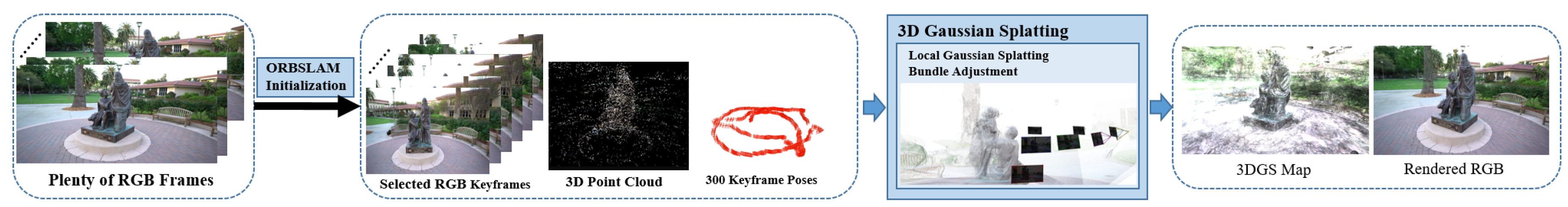
System Overview: The system starts with a large number of RGB frames and integrates two key processes: ORB-SLAM initialization and LGSBA, showing outstanding innovation. In the ORB-SLAM initialization stage, by using the advanced ORB-SLAM algorithm and comprehensively referring to multi-dimensional indicators such as scene change, feature point distribution and tracking quality, a small number of representative keyframes are accurately selected from a large number of RGB frames. This effectively simplifies the input system and reduces data redundancy. Subsequently, based on these selected keyframes, a 3D point cloud is constructed through precise feature matching and triangulation, and the poses of keyframes are accurately calculated to provide precise initial parameters for the subsequent 3DGS processing, greatly saving the initialization time. After entering the 3DGS training, it seamlessly takes over the results of the ORB-SLAM initialization and uses the 3DGS technology to discretize the scene into a Gaussian distribution form to build an initial 3D model. Particularly prominent is the innovative introduction of LGSBA process. This process utilizes the sliding window mechanism, focuses on the viewpoint optimization within the local window with the current viewpoint as the core, comprehensively considers indicators such as pixel-level differences and structural similarity, and iteratively adjusts the Gaussian parameters and poses through the loss function, significantly enhancing the rendering quality. Eventually, a high-precision 3DGS map and intuitive rendered RGB images are generated, bringing new breakthroughs to the 3DGS field.
Figure 1.
System Overview: The system starts with a large number of RGB frames and integrates two key processes: ORB-SLAM initialization and LGSBA, showing outstanding innovation. In the ORB-SLAM initialization stage, by using the advanced ORB-SLAM algorithm and comprehensively referring to multi-dimensional indicators such as scene change, feature point distribution and tracking quality, a small number of representative keyframes are accurately selected from a large number of RGB frames. This effectively simplifies the input system and reduces data redundancy. Subsequently, based on these selected keyframes, a 3D point cloud is constructed through precise feature matching and triangulation, and the poses of keyframes are accurately calculated to provide precise initial parameters for the subsequent 3DGS processing, greatly saving the initialization time. After entering the 3DGS training, it seamlessly takes over the results of the ORB-SLAM initialization and uses the 3DGS technology to discretize the scene into a Gaussian distribution form to build an initial 3D model. Particularly prominent is the innovative introduction of LGSBA process. This process utilizes the sliding window mechanism, focuses on the viewpoint optimization within the local window with the current viewpoint as the core, comprehensively considers indicators such as pixel-level differences and structural similarity, and iteratively adjusts the Gaussian parameters and poses through the loss function, significantly enhancing the rendering quality. Eventually, a high-precision 3DGS map and intuitive rendered RGB images are generated, bringing new breakthroughs to the 3DGS field.
4.3.1. Experiment 1: Comparison of ORB-SLAM and COLMAP Initialization
This group of experiments focuses on the initialization stage. We compare the initialization performance of COLMAP and ORB-SLAM using the TUM-RGBD, Tanks and Temples, and KITTI datasets. The results, summarized in Table 1, show that COLMAP requires a significantly longer time for sparse reconstruction and camera pose estimation (e.g., approximately 40 minutes for around 200 images) compared to ORB-SLAM, which reduces the initialization time to under 3 minutes.
Moreover, to assess the impact of the initialization method on 3DGS map optimization, we rendered the Gaussian maps generated under identical keyframe selection and pose conditions. In indoor scenarios (e.g., TUM-fg2 desk and TUM-fg3 long office), COLMAP yielded slightly higher PSNR values (by 0.91 dB and 0.73 dB, respectively) compared to ORB-SLAM. However, in outdoor or large-scale scenes (e.g., TANKS train, KITTI 00, TANKS m60, and TUM-fg1 floor), ORB-SLAM initialization produced notably better rendering results, with PSNR improvements of 3.04 dB, 6.52 dB, 2.11 dB, and 9.24 dB, respectively. On average, ORB-SLAM initialization achieved approximately 0.016 lower L1 loss, 1.6 dB higher PSNR, 0.051 higher SSIM, and 0.075 lower LPIPS than COLMAP, demonstrating its superiority in both speed and the quality of the generated Gaussian maps.
Figure 2.
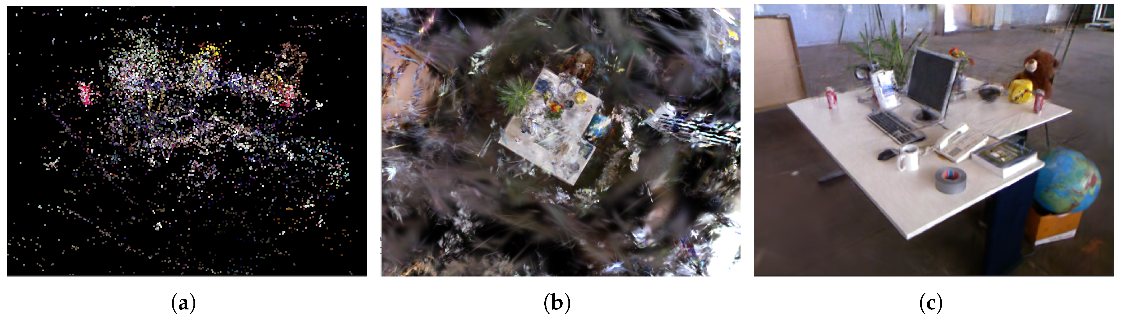
Different maps obtained from dataset TUM-fg2-desk with COLMAP initialization method and original 3DGS optimization. (a) Sparse point cloud from traditional SfM based system. (b) Gaussian map from 3DGS optimization. (c) Rendered image from Gaussian map with a specific viewpoint.
Figure 2.
Different maps obtained from dataset TUM-fg2-desk with COLMAP initialization method and original 3DGS optimization. (a) Sparse point cloud from traditional SfM based system. (b) Gaussian map from 3DGS optimization. (c) Rendered image from Gaussian map with a specific viewpoint.
4.3.2. Experiment 2: Comparison of Different 3DGS Training Methods
This experiment evaluates the robustness of the ORB-SLAM initialization and the performance gains achieved by incorporating the LGSBA optimization into the 3DGS training process. Starting from the same set of initial point clouds and camera poses provided by ORB-SLAM, we compare three training strategies: the original 3DGS training method, an advanced Scaffold-GS system, and our 3DGS training approach enhanced with LGSBA. The experiments were conducted on TUM-RGBD, Tanks and Temples, and KITTI datasets.
In the 3DGS map optimization phase, under identical keyframe and pose conditions, we rendered the Gaussian maps and evaluated them using PSNR, SSIM, LPIPS, and L1 loss. As detailed in Table 2, under 30,000 iterations, our LGSBA-enhanced method improved the PSNR by 2.17 dB, 0.29 dB, 10.4 dB, 4.38 dB, 5.73 dB, 1.82 dB, 2.15 dB, and 0.50 dB in various scenes (e.g., TUM-fg2 desk, TUM-fg3 long office, TUM-fg1 floor, Tanks Caterpillar, Tanks M60, Tanks Panther, Tanks Horse, and KITTI 00, respectively). Overall, compared to the original 3DGS training, the LGSBA method reduced the average L1 loss by approximately 0.012, increased PSNR by about 1.9 dB, improved SSIM by 0.068, and lowered LPIPS by 0.081. Similar improvements were observed when compared against the Scaffold-GS method. These results confirm that the high-quality initial point clouds and camera poses obtained via ORB-SLAM provide a solid foundation, and the LGSBA optimization significantly enhances the map quality and rendering fidelity, especially in outdoor and large-scale scenes.
Figure 3 showcases representative rendering results across multiple scenes using different initialization and training strategies, juxtaposed against the ground truth images. The first and second columns illustrate the outcomes of 3DGS trained with COLMAP and ORB-SLAM initialization, respectively, while the third and fourth columns display Scaffold-GS under the same initialization settings. In contrast, the fifth column presents our LGSBA-enhanced approach, and the last column shows the ground truth. Notably, our method exhibits more faithful reproduction of intricate geometric structures (e.g., the edges of machinery, detailed textures on the ground, and refined object boundaries) and more consistent color transitions. This superior fidelity is especially evident in outdoor or large-scale scenes (e.g., the excavator and sculpture models), where highly accurate camera poses and refined Gaussian parameters lead to sharper features and fewer rendering artifacts. Overall, these visual results corroborate the quantitative improvements reported in Table 2, underscoring the effectiveness of our LGSBA optimization in achieving high-quality 3DGS reconstructions.
4.3.3. Experiment 3: Evaluation of Camera Pose Accuracy and Rendering Details
This experiment assesses the impact of LGSBA optimization on camera pose accuracy and the rendering quality of the 3DGS map. We quantitatively evaluated the reconstructed camera poses using Absolute Pose Error (APE) and Root Mean Square Error (RMSE), and compared the optimized trajectories with the ground truth. For the TUM-RGBD dataset, high-precision ground-truth poses were obtained from a motion capture system; for the Tanks and Temples dataset, COLMAP-reconstructed trajectories served as the reference; and for the KITTI dataset, real poses were provided by a vehicle-mounted GPS-RTK system.
The results (see Table 3 and Figure 4) indicate that, in some indoor scenes (e.g., TUM-fg2 desk and TUM-fg3 long office), LGSBA slightly increased APE and RMSE compared to the poses estimated directly by ORB-SLAM. However, from the rendering perspective, LGSBA significantly improved the final image quality. For instance, in the TUM-fg2 desk scene, the PSNR improved from 25.40 dB to 26.37 dB, and in the TUM-fg3 long office scene, from 27.83 dB to 28.62 dB, highlighting that LGSBA effectively enhances rendering quality. Notably, in large outdoor scenes (e.g., KITTI and Tanks and Temples), the improvements were even more pronounced—with PSNR gains of up to 5.59 dB in the Tanks Caterpillar scene and 0.50 dB in the KITTI 00 scene.
In summary, although LGSBA may lead to a slight increase in physical pose error in certain scenarios, the overall enhancement in the rendered 3DGS map—reflected in improved visual quality and finer detail reconstruction—demonstrates its effectiveness. Figure 4 visually compares the optimized camera trajectories with the ground truth, providing further evidence of the rendering improvements brought about by LGSBA.
4.4. Online Integration of ORB-SLAM with 3DGS Map Optimization
4.4.1. System Overview:
In this experiment, we evaluate an online mapping system that tightly integrates ORB-SLAM with 3DGS optimization via our Local Gaussian Splatting Bundle Adjustment. As shown in Figure 5, the system leverages ORB-SLAM to perform real-time keyframe-based pose estimation and sparse point cloud generation, while the GSMaster node performs incremental optimization of a 3D Gaussian map. This online framework is implemented using the ROS distributed computing architecture, where separate nodes concurrently handle image preprocessing, SLAM processing, and 3DGS optimization.
4.4.2. Experimental Procedure:
The experiment is structured around the following key components:
- Real-Time Initialization and Data Flow: The system ingests preprocessed image streams (e.g., from a smartphone) published on the /camera/rgb topic. ORB-SLAM processes these images in real time by extracting features, estimating camera poses, and selecting keyframes based on tracking quality, parallax, and entropy thresholds. The resulting keyframes, poses, and sparse point clouds are published on dedicated topics (/slam/pose, /slam/pointcloud, and /slam/rgb) for subsequent 3DGS training.
- Incremental 3DGS Map Optimization using LGSBA: The GSMaster node subscribes to the SLAM outputs and initializes the 3DGS module by converting sparse points into Gaussian distributions, parameterized by mean , covariance , color c, and opacity . Before loop closure is detected, an incremental training mode is activated. In this mode, LGSBA refines both camera poses and Gaussian parameters using a sliding window that jointly minimizes a loss function—comprising L1 loss and error—across multiple keyframes. This dual-stage optimization balances pose accuracy with the rendered Gaussian map quality, enabling updated map renderings at 5–10 frames per second.
- Dynamic Training Mode Switching: When ORB-SLAM detects loop closure (indicated via the /slam/loop topic), the system automatically transitions from incremental to a global (random) training mode. In this phase, only the global 3D Gaussian map is optimized while camera poses remain fixed. This switch ensures global consistency and further refines rendering details by applying operations such as voxel downsampling and the removal of low-opacity Gaussians.
- Experimental Results: In a controlled laboratory environment, the online system was tested using an 80-second video captured at 1024×768 resolution and 30 FPS (downsampled to 15 FPS for processing). Out of approximately 1200 frames, ORB-SLAM selected 174 keyframes. Compared to an offline reconstruction pipeline, the online method dramatically reduced initialization time (from over 60 minutes of manual keyframe selection to under 3 minutes) while improving map quality. After 30,000 optimization iterations, the online method achieved average improvements of approximately +0.49 dB in PSNR, +0.013 in SSIM, and -0.042 in LPIPS over the offline baseline, all while maintaining real-time performance. Detailed experimental processes and visual results are shown in Figure 6, Figure 7, and Figure 8, with quantitative results summarized in Table 4.
4.4.3. Experimental Results Comparison:
To evaluate the performance of our proposed online 3DGS optimization method, we conduct a quantitative comparison with the offline reconstruction approach that utilizes ORB-SLAM for initialization, followed by 3DGS optimization. As shown in Table 4, our method achieves lower L1 error and LPIPS at 7K iterations, indicating improved perceptual quality. At 30K iterations, our approach maintains comparable L1 error while achieving slightly better PSNR and SSIM, demonstrating its effectiveness.
Unlike the quantitative analysis, we do not provide a direct qualitative comparison with the offline method. Instead, Figure 7 and Figure 8 present only the reconstruction results of our online approach. The Gaussian maps in Figure 7 illustrate the optimized 3D representation, while Figure 8 shows rendered images from multiple viewpoints, highlighting the structural and texture fidelity of our method.
However, since our system relies on ORB-SLAM for initialization, its robustness is affected in dynamic and low-texture environments. In such scenarios, inaccurate camera tracking degrades the reconstruction quality, which remains a limitation of our approach.
This experiment demonstrates that the online integration of ORB-SLAM with 3DGS optimization and LGSBA significantly enhances both the efficiency and quality of the mapping process. The system not only accelerates initialization and keyframe management but also produces high-quality 3D Gaussian maps suitable for real-time robotic applications.
5. Conclusion
In this article, we have made improvements to the original 3DGS system mainly in three aspects, including ORB-SLAM initialization, the introduction of LGSBA training, and the construction of a tightly coupled ORB-SLAM and 3DGS system. Eventually, we have managed to shorten the construction time by 10 times while improving the PSNR of the 3DGS map rendering. Based on our experiments, we have also discovered an interesting phenomenon: more accurate camera poses and point clouds in the physical world do not necessarily lead to the optimization of a 3DGS map of better quality, which is the core reason for our introduction of the LGSBA algorithm. We have also open-sourced the relevant source code of our work and some experimental results, which can be found at https://github.com/wla-98/worse-pose-but-better-3DGS.
However, our research lacks a more in-depth exploration of the better quality of camera poses and the optimization quality of 3DGS maps, which will be the core part of our future work.
Abbreviations
The following abbreviations are used in this manuscript:
| 3DGS | 3D Gaussian Splatting |
| BA | Bundle Adjustment |
| LGSBA | Local Gaussian Splatting Bundle Adjustment |
| ROS | Robot Operation System |
| NeRF | Neural Radiance Fields |
| SfM | Structure-from-Motion |
| SOTA | state-of-the-art |
| PSNR | Peak Signal-to-Noise Ratio |
| SSIM | Structural Similarity Index Measure |
| LPIPS | Learned Perceptual Image Patch Similarity |
| APE | Absolute Pose Error |
| RMSE | Root Mean Square Error |
| GT | Ground Truth |
References
- Kerbl, B.; Kopanas, G.; Leimkühler, T.; Drettakis, G. 3D Gaussian Splatting for Real-Time Radiance Field Rendering. ACM Trans. Graph. 2023, 42, 139–1. [Google Scholar] [CrossRef]
- Schonberger, J.L.; Frahm, J.M. Structure-from-motion revisited. 2016, pp. 4104–4113.
- Mildenhall, B.; Srinivasan, P.P.; Tancik, M.; Barron, J.T.; Ramamoorthi, R.; Ng, R. Nerf: Representing scenes as neural radiance fields for view synthesis. Communications of the ACM 2021, 65, 99–106. [Google Scholar] [CrossRef]
- Cheng, K.; Long, X.; Yang, K.; Yao, Y.; Yin, W.; Ma, Y.; Wang, W.; Chen, X. Gaussianpro: 3d gaussian splatting with progressive propagation. In Proceedings of the Forty-first International Conference on Machine Learning; 2024. [Google Scholar]
- Zhang, J.; Zhan, F.; Xu, M.; Lu, S.; Xing, E. Fregs: 3d gaussian splatting with progressive frequency regularization. 2024, pp. 21424–21433.
- Chung, J.; Oh, J.; Lee, K.M. Depth-regularized optimization for 3d gaussian splatting in few-shot images. 2024, pp. 811–820.
- Li, J.; Zhang, J.; Bai, X.; Zheng, J.; Ning, X.; Zhou, J.; Gu, L. Dngaussian: Optimizing sparse-view 3d gaussian radiance fields with global-local depth normalization. 2024, pp. 20775–20785.
- Zhu, Z.; Fan, Z.; Jiang, Y.; Wang, Z. Fsgs: Real-time few-shot view synthesis using gaussian splatting. In Proceedings of the European Conference on Computer Vision. Springer; 2025; pp. 145–163. [Google Scholar]
- Engel, J.; Koltun, V.; Cremers, D. Direct sparse odometry 2017. 40, 611–625.
- Engel, J.; Schöps, T.; Cremers, D. LSD-SLAM: Large-scale direct monocular SLAM. In Proceedings of the European conference on computer vision. Springer; 2014; pp. 834–849. [Google Scholar]
- Forster, C.; Pizzoli, M.; Scaramuzza, D. SVO: Fast semi-direct monocular visual odometry. IEEE, 2014, pp. 15–22.
- Newcombe, R.A.; Lovegrove, S.J.; Davison, A.J. DTAM: Dense tracking and mapping in real-time. IEEE, 2011, pp. 2320–2327.
- Mur-Artal, R.; Montiel, J.M.M.; Tardos, J.D. ORB-SLAM: a versatile and accurate monocular SLAM system 2015. 31, 1147–1163.
- Mur-Artal, R.; Tardós, J.D. Orb-slam2: An open-source slam system for monocular, stereo, and rgb-d cameras 2017. 33, 1255–1262.
- Campos, C.; Elvira, R.; Rodríguez, J.J.G.; Montiel, J.M.; Tardós, J.D. Orb-slam3: An accurate open-source library for visual, visual–inertial, and multimap slam 2021. 37, 1874–1890.
- Ragot, N.; Khemmar, R.; Pokala, A.; Rossi, R.; Ertaud, J.Y. Benchmark of visual slam algorithms: Orb-slam2 vs rtab-map. In Proceedings of the 2019 Eighth International Conference on Emerging Security Technologies (EST). IEEE, 2019, pp. 1–6.
- Qin, T.; Li, P.; Shen, S. Vins-mono: A robust and versatile monocular visual-inertial state estimator 2018. 34, 1004–1020.
- Klein, G.; Murray, D. Parallel tracking and mapping for small AR workspaces. In Proceedings of the 2007 6th IEEE and ACM international symposium on mixed and augmented reality. IEEE, 2007, pp. 225–234.
- Zhu, Z.; Peng, S.; Larsson, V.; Xu, W.; Bao, H.; Cui, Z.; Oswald, M.R.; Pollefeys, M. Nice-slam: Neural implicit scalable encoding for slam. 2022, pp. 12786–12796.
- Rosinol, A.; Leonard, J.J.; Carlone, L. Nerf-slam: Real-time dense monocular slam with neural radiance fields. IEEE, 2023, pp. 3437–3444.
- Zhu, Z.; Peng, S.; Larsson, V.; Cui, Z.; Oswald, M.R.; Geiger, A.; Pollefeys, M. Nicer-slam: Neural implicit scene encoding for rgb slam. In Proceedings of the 2024 International Conference on 3D Vision (3DV). IEEE; 2024; pp. 42–52. [Google Scholar]
- Kong, X.; Liu, S.; Taher, M.; Davison, A.J. vmap: Vectorised object mapping for neural field slam. 2023, pp. 952–961.
- Sandström, E.; Li, Y.; Van Gool, L.; Oswald, M.R. Point-slam: Dense neural point cloud-based slam. 2023, pp. 18433–18444.
- Chung, C.M.; Tseng, Y.C.; Hsu, Y.C.; Shi, X.Q.; Hua, Y.H.; Yeh, J.F.; Chen, W.C.; Chen, Y.T.; Hsu, W.H. Orbeez-slam: A real-time monocular visual slam with orb features and nerf-realized mapping. IEEE, 2023, pp. 9400–9406.
- Huang, H.; Li, L.; Cheng, H.; Yeung, S.K. Photo-SLAM: Real-time Simultaneous Localization and Photorealistic Mapping for Monocular Stereo and RGB-D Cameras. 2024, pp. 21584–21593.
- Yugay, V.; Li, Y.; Gevers, T.; Oswald, M.R. Gaussian-slam: Photo-realistic dense slam with gaussian splatting. arXiv preprint arXiv:2312.10070, 2023. [Google Scholar]
- Yan, C.; Qu, D.; Xu, D.; Zhao, B.; Wang, Z.; Wang, D.; Li, X. Gs-slam: Dense visual slam with 3d gaussian splatting. 2024, pp. 19595–19604.
- Li, M.; Liu, S.; Zhou, H.; Zhu, G.; Cheng, N.; Deng, T.; Wang, H. Sgs-slam: Semantic gaussian splatting for neural dense slam. In Proceedings of the European Conference on Computer Vision. Springer; 2025; pp. 163–179. [Google Scholar]
- Keetha, N.; Karhade, J.; Jatavallabhula, K.M.; Yang, G.; Scherer, S.; Ramanan, D.; Luiten, J. SplaTAM: Splat Track & Map 3D Gaussians for Dense RGB-D SLAM. 2024, pp. 21357–21366.
- Ji, Y.; Liu, Y.; Xie, G.; Ma, B.; Xie, Z. Neds-slam: A novel neural explicit dense semantic slam framework using 3d gaussian splatting. arXiv preprint arXiv:2403.11679, 2024. [Google Scholar]
- Liu, Y.; Dong, S.; Wang, S.; Yin, Y.; Yang, Y.; Fan, Q.; Chen, B. SLAM3R: Real-Time Dense Scene Reconstruction from Monocular RGB Videos. arXiv preprint arXiv:2412.09401, 2024. [Google Scholar]
- Smart, B.; Zheng, C.; Laina, I.; Prisacariu, V.A. Splatt3R: Zero-shot Gaussian Splatting from Uncalibrated Image Pairs 2024. [arXiv:cs.CV/2408.13912].
- Teed, Z.; Deng, J. DROID-SLAM: Deep Visual SLAM for Monocular, Stereo, and RGB-D Cameras. Advances in neural information processing systems 2021. [Google Scholar]
- Wang, S.; Leroy, V.; Cabon, Y.; Chidlovskii, B.; Revaud, J. Dust3r: Geometric 3d vision made easy. 2024, pp. 20697–20709.
- Matsuki, H.; Murai, R.; Kelly, P.H.; Davison, A.J. Gaussian splatting slam. 2024, pp. 18039–18048.
- Zwicker, M.; Pfister, H.; Van Baar, J.; Gross, M. EWA volume splatting. In Proceedings of the Proceedings Visualization, 2001. VIS’01. IEEE, 2001, pp. 29–538.
- Lu, T.; Yu, M.; Xu, L.; Xiangli, Y.; Wang, L.; Lin, D.; Dai, B. Scaffold-gs: Structured 3d gaussians for view-adaptive rendering. 2024, pp. 20654–20664.
Figure 3.
Qualitative comparison of 3DGS reconstructions across different scenes. Each row presents rendering results for different datasets: Tank-horse, Caterpillar, Family, and Floor. In each case, we compare the outputs of 3DGS initialized with COLMAP and ORB-SLAM, as well as alternative approaches. The images demonstrate that our method consistently produces sharper details, smoother textures, and fewer artifacts, particularly in challenging scenarios with complex structures and occlusions. Notably, fine-grained features such as object contours, surface textures, and depth variations are better preserved, reinforcing the efficacy of our proposed initialization and optimization strategies.
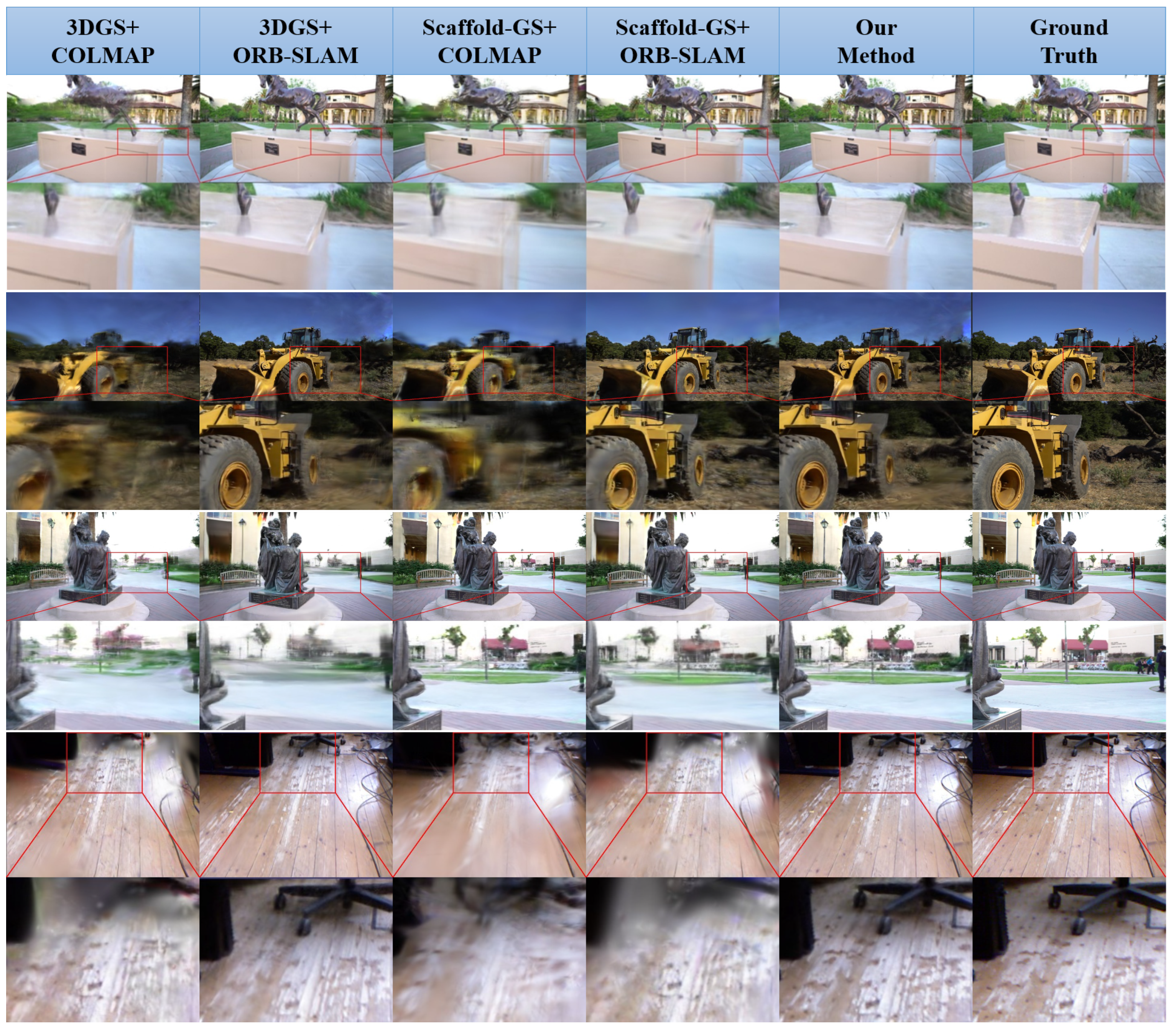
Figure 4.
Comparison of estimated trajectories before and after LGSBA optimization across different datasets. Each subfigure presents three trajectories: the ground truth, the trajectory before LGSBA optimization, and the trajectory after LGSBA optimization. The GT trajectories are obtained differently for each dataset: (a)-(f) use motion capture (MoCap) system data from the TUM dataset, (g) uses COLMAP-generated poses as GT in the TANKS dataset, and (h) uses GPS-RTK data for KITTI. All estimated trajectories are initialized using ORB-SLAM. While LGSBA does not improve trajectory accuracy, as shown in these comparisons, previous experiments demonstrate that it produces higher-quality Gaussian maps. (a) TUM-fg1-xyz. (b) TUM-fg1-desk. (c) TUM-fg1-floor. (d) TUM-fg2-desk-orb. (e) TUM-fg2-large-loop. (f) TUM-fg3-long-office-household. (g) TANKS-family. (h) KITTI.
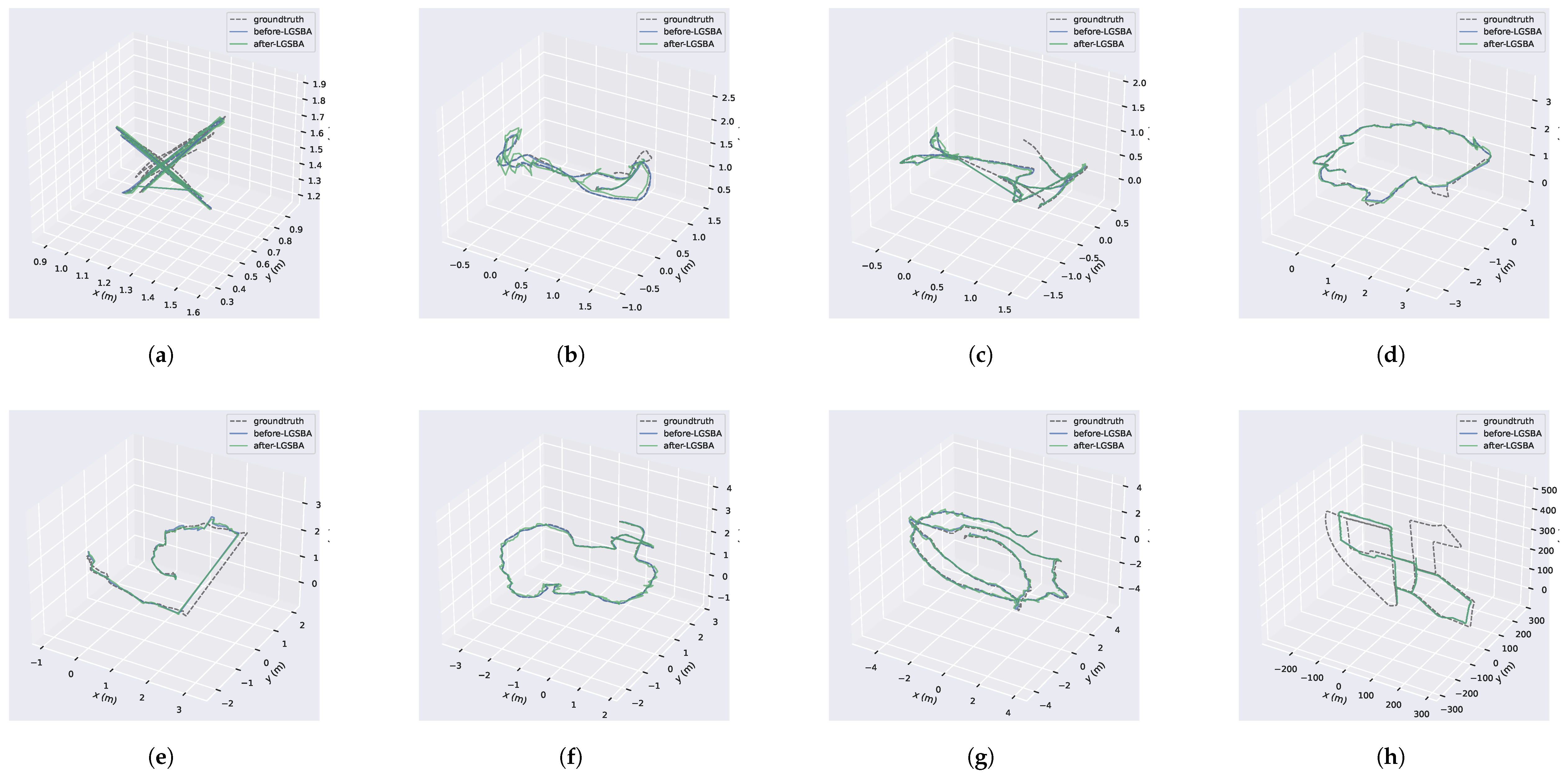
Figure 5.
System Overview: Our online optimization system achieves tight coupling between ORB-SLAM3 and the 3DGS system through ROS. By leveraging ORB-SLAM3, we optimize the number of input images to extract keyframes and simultaneously solve for the poses of these keyframes along with a sparse point cloud map. Using ROS nodes, the Local Mapping thread of ORB-SLAM3 publishes real-time results of local bundle adjustment(BA) optimization including keyframes’ images, keyframes’ poses and keyframes’ mappoints, which are then fed into the 3DGS system to enable incremental scene construction and updates. Additionally, we utilize the Loop Closing thread of ORB-SLAM3 to perform global BA. Upon completion of the global BA, we introduce randomly selected scene cameras for training, thereby enhancing the system’s robustness and improving the quality of 3DGS map reconstruction.
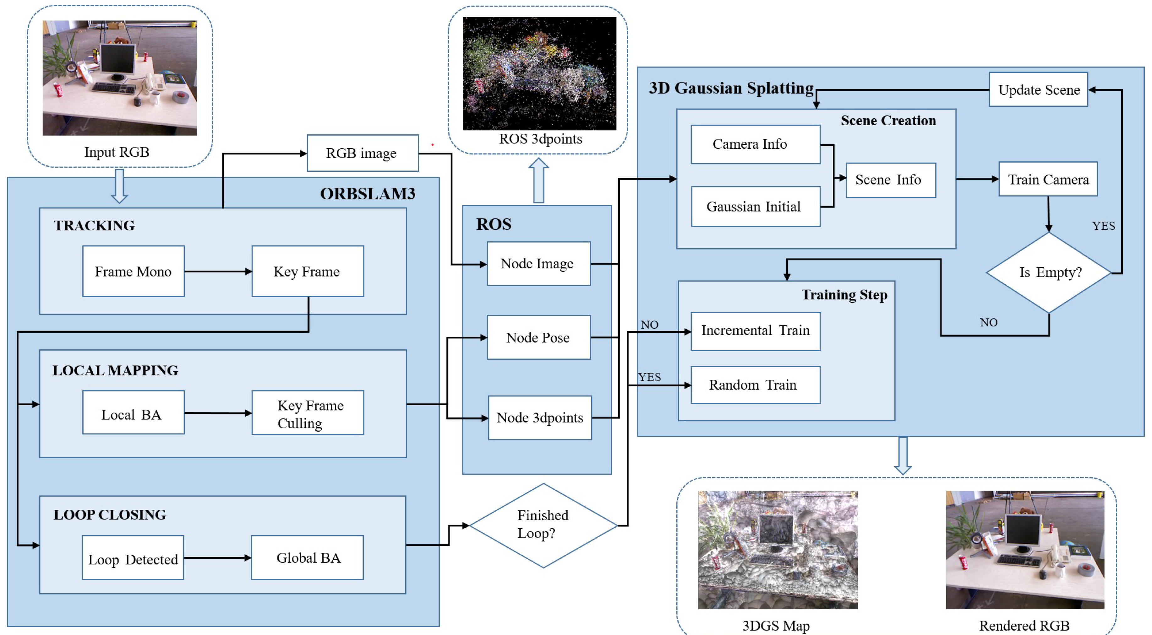
Figure 6.
Lab point cloud and camera poses generated by ORB-SLAM for 3DGS optimization.
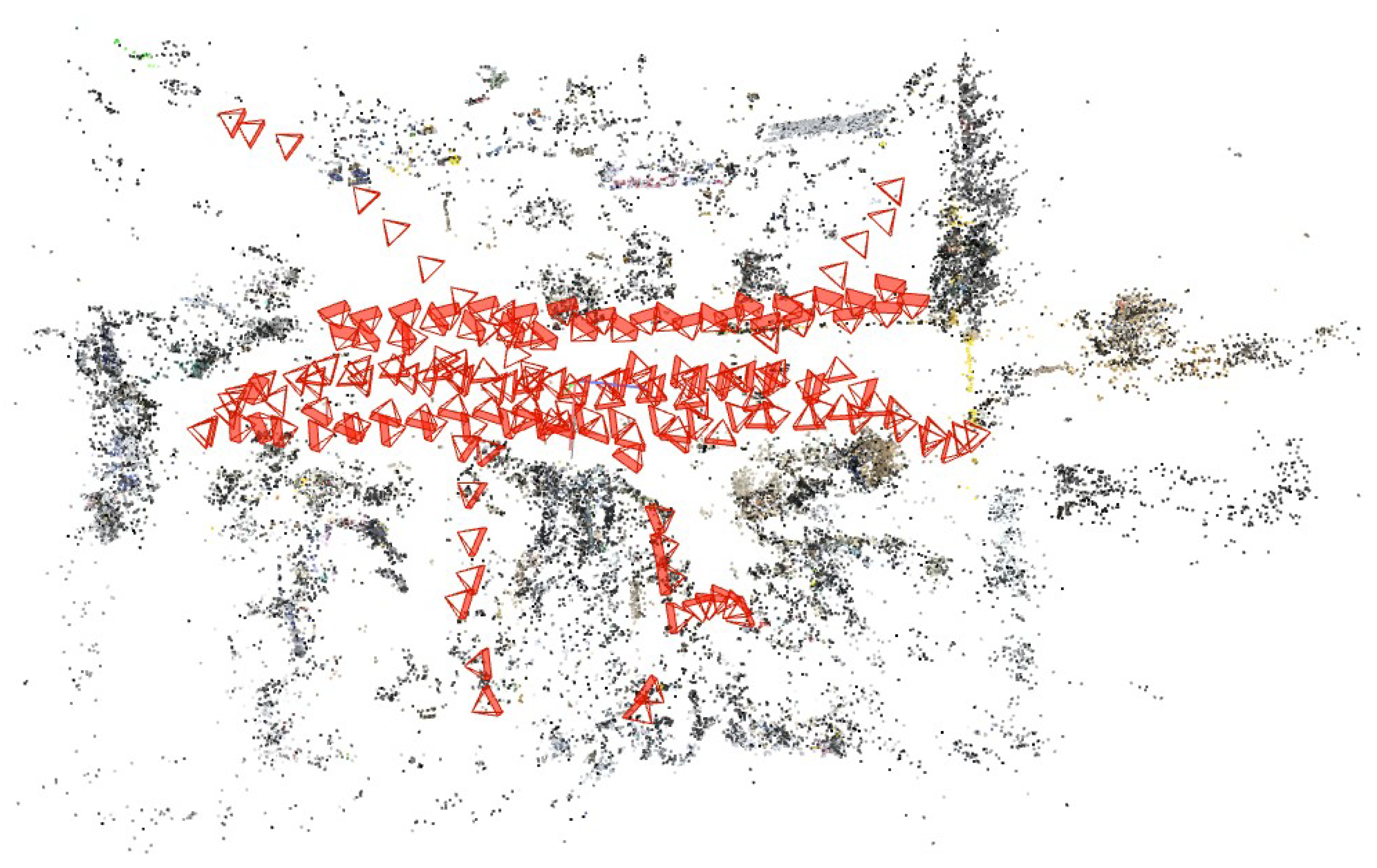
Figure 7.
Gaussian maps observed from different viewpoints.
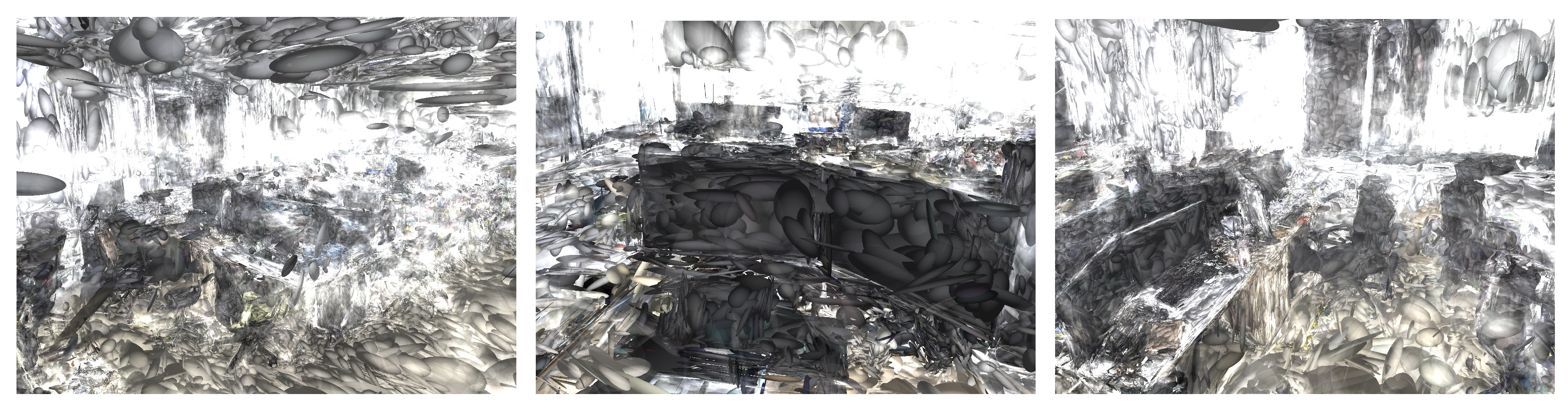
Figure 8.
Rendered images obtained from the Gaussian map, shown from six different viewpoints.
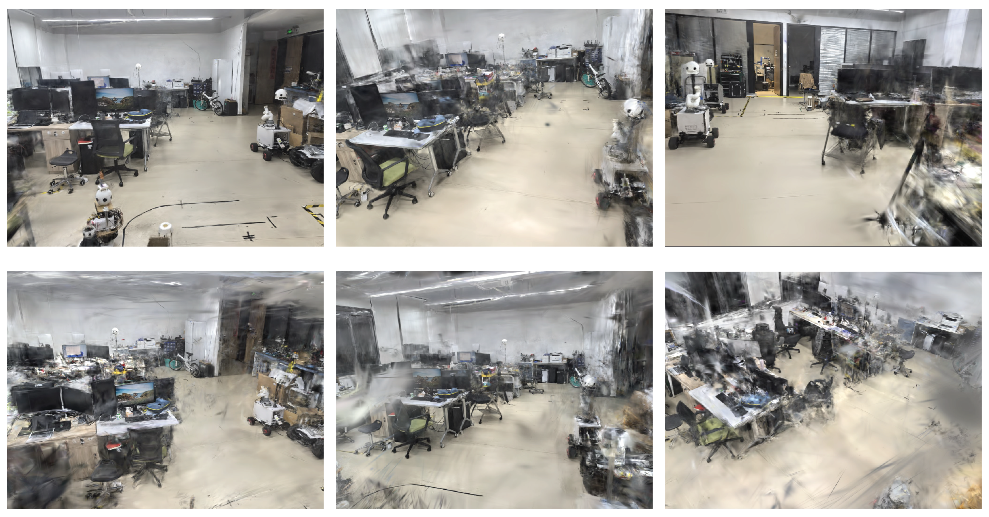

Table 1.
Comparative evaluation of 3DGS reconstruction performance using two initialization methods: COLMAP-based offline initialization (requiring >40,min) versus ORB-SLAM-based offline initialization (<3,min). The table reports quantitative results across multiple scenes from the TUM-RGBD, Tanks & Temples, and KITTI datasets at two training iteration levels (7K and 30K). Evaluation metrics include L1 pixel error (lower is better), PSNR (dB, higher is better), SSIM (higher is better), and LPIPS (lower is better). The final row provides average values across all scenarios, demonstrating that ORB-SLAM-based initialization not only drastically reduces initialization time but also achieves competitive or superior reconstruction quality compared to the COLMAP-based approach, specifically as illustrated in Section 4.3.1.
| Scenes | Iterations | 3DGS w. COLMAP (>40min) | 3DGS w. ORB-SLAM (<3min) | ||||||
| L1 ↓ | PSNR ↑ | SSIM ↑ | LPIPS ↓ | L1 ↓ | PSNR ↑ | SSIM ↑ | LPIPS ↓ | ||
| TUM-fg2 | 7000 | 0.05144 | 21.9198 | 0.7304 | 0.3490 | 0.04445 | 22.7231 | 0.7398 | 0.3392 |
| desk | 30000 | 0.02692 | 26.3146 | 0.8140 | 0.2534 | 0.03106 | 25.4048 | 0.8079 | 0.2526 |
| TUM-fg3 | 7000 | 0.02768 | 26.6919 | 0.8828 | 0.2006 | 0.02967 | 25.9192 | 0.8702 | 0.2132 |
| long office | 30000 | 0.02158 | 28.5634 | 0.9013 | 0.1729 | 0.02271 | 27.8335 | 0.8962 | 0.1739 |
| TUM-fg2 | 7000 | 0.09013 | 16.6208 | 0.6753 | 0.4117 | 0.06844 | 18.6592 | 0.7093 | 0.3832 |
| large loop | 30000 | 0.03953 | 22.3948 | 0.8221 | 0.2708 | 0.03502 | 23.5877 | 0.8487 | 0.2321 |
| TUM-fg1 | 7000 | 0.08924 | 17.3659 | 0.6043 | 0.5873 | 0.04084 | 24.1946 | 0.7139 | 0.4045 |
| floor | 30000 | 0.06791 | 19.4411 | 0.6449 | 0.5265 | 0.02246 | 28.6884 | 0.8123 | 0.2447 |
| TUM-fg1 | 7000 | 0.04417 | 21.8245 | 0.7884 | 0.3341 | 0.04271 | 21.7174 | 0.8032 | 0.3109 |
| desk | 30000 | 0.02568 | 26.1006 | 0.8737 | 0.2388 | 0.02467 | 26.6830 | 0.8783 | 0.2234 |
| L1 ↓ | PSNR ↑ | SSIM ↑ | LPIPS ↓ | L1 ↓ | PSNR ↑ | SSIM ↑ | LPIPS ↓ | ||
| TANKS | 7000 | 0.07256 | 18.1196 | 0.5255 | 0.5333 | 0.07196 | 18.4721 | 0.6110 | 0.4194 |
| family | 30000 | 0.05623 | 19.8652 | 0.6159 | 0.4277 | 0.05907 | 19.9479 | 0.6985 | 0.3254 |
| TANKS | 7000 | 0.11464 | 15.1700 | 0.3834 | 0.6885 | 0.09600 | 16.6443 | 0.4398 | 0.6024 |
| caterpillar | 30000 | 0.08644 | 17.1147 | 0.4377 | 0.6035 | 0.07899 | 17.8833 | 0.4994 | 0.5322 |
| TANKS | 7000 | 0.06237 | 19.4507 | 0.6307 | 0.5360 | 0.04580 | 21.1421 | 0.7017 | 0.4393 |
| m60 | 30000 | 0.04873 | 21.1488 | 0.6869 | 0.4582 | 0.03388 | 23.1617 | 0.7808 | 0.3381 |
| TANKS | 7000 | 0.04526 | 22.1129 | 0.6982 | 0.5100 | 0.06553 | 19.7737 | 0.6387 | 0.4786 |
| panther | 30000 | 0.03464 | 24.1963 | 0.7557 | 0.4325 | 0.05116 | 21.5959 | 0.7051 | 0.3954 |
| TANKS | 7000 | 0.04773 | 19.9960 | 0.7077 | 0.3804 | 0.03704 | 22.3863 | 0.7689 | 0.2957 |
| horse | 30000 | 0.03387 | 22.3492 | 0.7786 | 0.2897 | 0.029178 | 24.2530 | 0.8263 | 0.2284 |
| TANKS | 7000 | 0.10385 | 15.7136 | 0.4410 | 0.6150 | 0.07377 | 18.7738 | 0.5714 | 0.4680 |
| train | 30000 | 0.07547 | 17.9350 | 0.5541 | 0.4793 | 0.05424 | 20.9735 | 0.6781 | 0.3498 |
| TANKS | 7000 | 0.09312 | 18.8726 | 0.6620 | 0.4513 | 0.04761 | 20.8189 | 0.7084 | 0.3546 |
| lighthouse | 30000 | 0.04949 | 21.8844 | 0.7152 | 0.4086 | 0.03683 | 22.7946 | 0.7728 | 0.2814 |
| KITTI | 7000 | 0.18991 | 11.1005 | 0.4582 | 0.6040 | 0.14224 | 13.3166 | 0.5003 | 0.5895 |
| 00 | 30000 | 0.17236 | 11.5722 | 0.4701 | 0.5991 | 0.07117 | 18.0943 | 0.5973 | 0.5340 |
| Average | 0.06811 | 20.1477 | 0.6638 | 0.4370 | 0.05217 | 21.7478 | 0.7146 | 0.3619 | |
* ↓ indicates lower is better, ↑ indicates higher is better.
Table 2.
Comparative evaluation of 3DGS reconstruction quality using three methods: (1) 3DGS with ORB-SLAM initialization, (2) Scaffold-GS[37] with ORB-SLAM initialization, and (3) our proposed method. The table reports quantitative results on various challenging scenes from TUM-RGBD, Tanks & Temples, and KITTI datasets at two training iteration counts (7K and 30K). Metrics include L1 pixel error, PSNR, SSIM , and LPIPS. Best results per metric-scenario combination are highlighted in deep red. This comprehensive evaluation demonstrates that our method consistently outperforms the other approaches, achieving superior perceptual quality (indicated by higher PSNR and SSIM, and lower L1 and LPIPS across a diverse set of scenes, specifically as illustrated in Section 4.3.2.
| Scenes | Iterations | 3DGS w. ORB-SLAM | Scaffold-GS[37] w. ORB-SLAM | Our Method | |||||||||
| L1 ↓ | PSNR ↑ | SSIM ↑ | LPIPS ↓ | L1 ↓ | PSNR ↑ | SSIM ↑ | LPIPS ↓ | L1 ↓ | PSNR ↑ | SSIM ↑ | LPIPS ↓ | ||
| TUM-fg2 | 7000 | 0.04445 | 22.7231 | 0.7398 | 0.3392 | 0.05892 | 19.5031 | 0.6562 | 0.3605 | 0.04147 | 23.2687 | 0.7564 | 0.3190 |
| desk | 30000 | 0.03106 | 25.4048 | 0.8079 | 0.2526 | 0.03963 | 24.1913 | 0.7816 | 0.2749 | 0.02675 | 26.3698 | 0.8215 | 0.2366 |
| TUM-fg3 | 7000 | 0.02967 | 25.9192 | 0.8702 | 0.2132 | 0.03046 | 26.1320 | 0.8495 | 0.2171 | 0.02788 | 26.6086 | 0.8754 | 0.1790 |
| long office | 30000 | 0.02271 | 27.8335 | 0.8962 | 0.1739 | 0.02254 | 28.3261 | 0.8871 | 0.1710 | 0.02148 | 28.6190 | 0.9029 | 0.1448 |
| TUM-fg2 | 7000 | 0.06844 | 18.6592 | 0.7093 | 0.3832 | 0.04203 | 22.7576 | 0.8250 | 0.3370 | 0.06613 | 18.4161 | 0.7306 | 0.3476 |
| large loop | 30000 | 0.03502 | 23.5877 | 0.8487 | 0.2321 | 0.02675 | 26.5550 | 0.8923 | 0.2297 | 0.03297 | 23.9026 | 0.8613 | 0.2121 |
| TUM-fg1 | 7000 | 0.04084 | 24.1946 | 0.7139 | 0.4045 | 0.11536 | 16.4651 | 0.5028 | 0.5832 | 0.03785 | 24.7616 | 0.7615 | 0.2751 |
| floor | 30000 | 0.02246 | 28.6884 | 0.8123 | 0.2447 | 0.08608 | 18.8924 | 0.5747 | 0.4874 | 0.02111 | 29.2896 | 0.8756 | 0.1493 |
| TUM-fg1 | 7000 | 0.04271 | 21.7174 | 0.8032 | 0.3109 | 0.02675 | 26.2993 | 0.8503 | 0.2593 | 0.03837 | 22.9983 | 0.8162 | 0.2823 |
| desk | 30000 | 0.02467 | 26.6830 | 0.8783 | 0.2234 | 0.01646 | 30.6417 | 0.9160 | 0.1568 | 0.02117 | 28.1143 | 0.8954 | 0.1827 |
| TANKS | 7000 | 0.07196 | 18.4721 | 0.6110 | 0.4194 | 0.06984 | 18.6930 | 0.5614 | 0.5110 | 0.03922 | 23.3886 | 0.7625 | 0.2996 |
| family | 30000 | 0.05907 | 19.9479 | 0.6985 | 0.3254 | 0.05224 | 20.6179 | 0.6758 | 0.3822 | 0.02978 | 24.9964 | 0.8308 | 0.2174 |
| TANKS | 7000 | 0.09600 | 16.6443 | 0.4398 | 0.6024 | 0.07732 | 18.4520 | 0.4906 | 0.5410 | 0.04741 | 22.7639 | 0.5953 | 0.4220 |
| Caterpillar | 30000 | 0.07899 | 17.8833 | 0.4994 | 0.5322 | 0.06325 | 19.8104 | 0.5540 | 0.4780 | 0.02791 | 25.5355 | 0.7991 | 0.2577 |
| TANKS | 7000 | 0.04580 | 21.1421 | 0.7017 | 0.4393 | 0.05177 | 20.7905 | 0.6669 | 0.4058 | 0.03578 | 22.2298 | 0.7901 | 0.3279 |
| M60 | 30000 | 0.03388 | 23.1617 | 0.7808 | 0.3381 | 0.03472 | 23.8326 | 0.7897 | 0.2907 | 0.02820 | 23.7872 | 0.8426 | 0.2699 |
| TANKS | 7000 | 0.06553 | 19.7737 | 0.6387 | 0.4786 | 0.05711 | 20.6153 | 0.6727 | 0.4603 | 0.05074 | 21.1269 | 0.6978 | 0.3882 |
| Panther | 30000 | 0.05116 | 21.5959 | 0.7051 | 0.3954 | 0.03952 | 23.4914 | 0.7759 | 0.3586 | 0.04139 | 22.7304 | 0.7591 | 0.3242 |
| TANKS | 7000 | 0.03704 | 22.3863 | 0.7689 | 0.2957 | 0.05187 | 20.8398 | 0.7611, | 0.3327 | 0.02885 | 25.0431 | 0.8344 | 0.2404 |
| Horse | 30000 | 0.029178 | 24.2530 | 0.8263 | 0.2284 | 0.03315 | 24.6180 | 0.8305 | 0.2537 | 0.02376 | 26.4398 | 0.8703 | 0.1921 |
| TANKS | 7000 | 0.07377 | 18.7738 | 0.5714 | 0.4680 | 0.06106 | 19.5181 | 0.6711 | 0.3860 | 0.04691 | 21.4430 | 0.7350 | 0.2839 |
| Train | 30000 | 0.05424 | 20.9735 | 0.6781 | 0.3498 | 0.05012 | 20.9398 | 0.7425 | 0.3110 | 0.03743 | 23.0867 | 0.8009 | 0.2146 |
| TANKS | 7000 | 0.04761 | 20.8189 | 0.7084 | 0.3546 | 0.03904 | 22.5495 | 0.7917 | 0.3203 | 0.03289 | 22.9611 | 0.8092 | 0.2290 |
| Lighthouse | 30000 | 0.03683 | 22.7946 | 0.7728 | 0.2814 | 0.02433 | 26.3856 | 0.8633 | 0.2332 | 0.02426 | 25.0581 | 0.8507 | 0.1863 |
| KITTI | 7000 | 0.14224 | 13.3166 | 0.5003 | 0.5895 | 0.13359 | 14.1273 | 0.4716 | 0.6247 | 0.14586 | 13.2683 | 0.4808 | 0.6128 |
| 00 | 30000 | 0.07117 | 18.0943 | 0.5973 | 0.5340 | 0.08427 | 17.3860 | 0.5659 | 0.5334 | 0.06340 | 18.5983 | 0.6029 | 0.5117 |
| Average | 0.05217 | 21.7478 | 0.7146 | 0.3619 | 0.05339 | 22.0166 | 0.7144 | 0.3654 | 0.03996 | 23.6464 | 0.7830 | 0.2810 | |
Table 3.
Quantitative evaluation of pose estimation and rendering quality across different datasets. The table presents APE and RMSE for pose estimation, along with PSNR for rendering quality. Results are reported for multiple datasets, including TUM-fg2, TUM-fg1, KITTI-00, and TANKS (Family, Caterpillar). Lower APE and RMSE values indicate more accurate pose estimation, while higher PSNR values reflect better rendering quality. The comparison highlights the effectiveness of different methods in handling diverse scenes with varying levels of complexity and motion
| Pose Estimation |
Metric | TUM-fg2 | TUM-fg1 | Others | ||||||
| desk | long office |
large w. loop |
xyz | floor | desk | KITTI-00 | TANKS-Family | TANKS-Caterpillar | ||
| Pose Estimation |
APE (cm) ↓ | 0.4590 | 0.8744 | 7.0576 | 0.6736 | 9.2631 | 1.3382 | 14.3767 | 13.0878 | 0.1005 |
| RMSE (cm) ↓ | 0.4962 | 0.9844 | 8.5865 | 0.7624 | 10.8200 | 1.5237 | 17.4024 | 15.5307 | 0.1074 | |
| APE (cm) ↓ | 4.1687 | 8.0663 | 7.7640 | 1.0193 | 3.4214 | 2.1502 | 14.4333 | 17.5868 | 0.1003 | |
| RMSE (cm) ↓ | 4.9558 | 9.0545 | 8.9127 | 1.0869 | 4.1349 | 2.9608 | 17.4314 | 20.6191 | 0.1070 | |
| Quality | PSNR ↑ | 25.4048 | 27.8335 | 23.5877 | 28.1725 | 28.6884 | 26.6830 | 18.0943 | 19.9479 | 17.8833 |
| PSNR ↑ | 26.3698 | 28.6190 | 23.9026 | 28.5573 | 29.2896 | 28.1143 | 18.5983 | 24.9964 | 25.5355 | |
* ↓ indicates lower is better, ↑ indicates higher is better.
Table 4.
Comparative evaluation of offline reconstruction (ORB-SLAM initialization with 3DGS optimization) versus our improved online reconstruction method in a laboratory indoor scene.
Table 4.
Comparative evaluation of offline reconstruction (ORB-SLAM initialization with 3DGS optimization) versus our improved online reconstruction method in a laboratory indoor scene.
| Scene | Iterations | Offline Reconstruction | Online Reconstruction (Ours) | ||||||
| L1 ↓ | PSNR ↑ | SSIM ↑ | LPIPS ↓ | L1 ↓ | PSNR ↑ | SSIM ↑ | LPIPS ↓ | ||
| Lab | 7K | 0.0575 | 21.20 | 0.775 | 0.363 | 0.0467 | 21.47 | 0.778 | 0.333 |
| 30K | 0.0297 | 24.15 | 0.858 | 0.276 | 0.0299 | 24.65 | 0.870 | 0.234 | |
* ↓ indicates lower is better, ↑ indicates higher is better.
Disclaimer/Publisher’s Note: The statements, opinions and data contained in all publications are solely those of the individual author(s) and contributor(s) and not of MDPI and/or the editor(s). MDPI and/or the editor(s) disclaim responsibility for any injury to people or property resulting from any ideas, methods, instructions or products referred to in the content. |
© 2025 by the authors. Licensee MDPI, Basel, Switzerland. This article is an open access article distributed under the terms and conditions of the Creative Commons Attribution (CC BY) license (http://creativecommons.org/licenses/by/4.0/).
Copyright: This open access article is published under a Creative Commons CC BY 4.0 license, which permit the free download, distribution, and reuse, provided that the author and preprint are cited in any reuse.


