Submitted:
09 May 2025
Posted:
12 May 2025
You are already at the latest version
Abstract
The increasing anthropogenic pressures on rural landscapes, particularly those arising from agricultural intensification, necessitate robust methods to assess environmental sustainability. This study proposes a multi-criteria approach for evaluating the environmental sustainability of rural landscape in northern Benin, using satellite-derived land cover data. The methodology was applied to 3 sites representative of rural landscapes in northern Benin. A 12-class land cover map, produced via the Moringa processing chain, was reclassified into Human Disturbance Coefficients (HDC) based on nine weighted environmental impact criteria. These were then spatially aggregated into 1 km² grid cells to produce the Landscape Environmental Sustainability Index (LESI). Results indicate that most areas exhibit moderate anthropogenic impact (HDC and LESI values between 2.5 and 3.5), covering 63–75% (HDC) and 83–94% (LESI) of the respective sites. Areas of low impact (values between 1.5 and 2.5) account for 20–24% (HDC) and 5–13% (LESI). The LESI, derived from accessible and cost-effective satellite data, offers a scalable, reproducible, and spatially explicit tool for monitoring landscape sustainability. It holds potential for guiding territorial governance and supporting transitions towards more sustainable land management practices. Future improvements may include refining evaluation criteria and introducing variable weighting schemes by land cover or region.
Keywords:
ecological sustainability
; agroecosystems
; satellite remote sensing
; anthropogenic pressures
; landscape resilience
; Northern Benin
1. Introduction
Driven by population growth and rising per capita incomes, global demand for agricultural products has increased significantly and is projected to continue growing in the coming decades [1]. Sub-Saharan Africa, as one of the fastest-growing regions globally, must considerably increase its agricultural output to meet current and future food demand [2]. Traditional strategies to boost production—such as intensifying yields per hectare, adopting intensive tillage practices, applying chemical fertilisers, and expanding farmland through deforestation—have led to substantial negative environmental externalities, including biodiversity loss [3], ecosystem service degradation, increased greenhouse gas emissions [4], and terrestrial and marine pollution [5].
The growing anthropogenic pressure on rural landscapes and in particular the increase in negative environmental externalities induced by the intensification of agriculture in response to the rise in demand for agricultural products, underscores the need to monitor environmental dynamics and provide land managers with accurate tools to assess and mitigate degradation [6]. Effective monitoring relies on the identification of relevant indicators [7]. Several initiatives have led to the development of a variety of indicators [8]. Calculating these indicators often requires costly and recurrent field surveys [7,9]. The cost of implementing these surveys, the challenges of ensuring that the results are representative, and the biases in the collection of the data all limit the computation of the indicators. [10]. Advances in remote sensing—particularly the increasing availability of free imagery with high spectral, spatial, and temporal resolution—offer cost-effective, scalable alternatives to overcome these challenges [11]. Satellite and airborne remote sensing provide up-to-date spatio-temporal data that can be used to quantify certain anthropogenic impacts on land, and in particular to assess certain negative environmental externalities associated with agriculture and its intensification, at various scales (landscape, region, etc.), by calculating indicators [12,13].
Several spatial indicators derived from remote sensing have been proposed to assess anthropogenic pressure, including the hemeroby index [14], agroecosystem quality index [15], landscape ecological security index [16], ecosystem health index [17], and farmland quality index [18]. Among these, the hemeroby index evaluates the degree of deviation from natural state due to human activity [19]. Thus, according to Sukopp [14], quoted by Walz and Stein [19], the hemeroby index is an integrated measure of the impact of human activities on ecosystems.
The hemeroby index is generally obtained by classifying remotely sensed images into land cover classes, which are then reclassified into categories reflecting the level of hemeroby. There are two approaches to this reclassification. The first approach consists of directly associating each land cover class with a predefined hemeroby class typically varying from 1 (no negative environmental externalities) to 7 (maximum intensity negative environmental externalities) [19,20,21,22,23]. The direct association of a land cover class with a hemeroby class is based on the intensity, duration and extent of the negative environmental externalities [24] that are observed in the said land cover class. The second reclassification approach initially involves calculating a hemeroby value for each land cover class, which may (i) be the result of a multi-criteria analysis based on the aggregation, by arithmetic mean, of scores assessed for a series of criteria and metrics (or sub-criteria) [25], or (ii) correspond to an ‘anthropisation coefficient’ obtained from existing reports and a simple expert rating [26,27]. The hemeroby value calculated in this way is then associated with a hemeroby class. It should be noted, however, that the hemeroby index does not take into account all negative environmental externalities that may be associated with the different land cover classes (greenhouse gas emissions, biodiversity erosion, etc.) [25].
Concerning the presentation and communication of the hemeroby index derived from land cover classes, some are subject to spatial aggregation on a larger scale than the initial calculation scale (pixel scale), which may typically correspond to a regular grid (e.g. 1km or 5km square), administrative boundaries, landscape entities, etc. The aggregation is generally carried out, for each target spatial entity, in the form of a sum of the indicator values relating to each land cover class, weighted by the percentage of surface area of each class. Aggregation is typically performed, for each target spatial feature, as a sum of the indicator values related to each land cover class, weighted by the areal percentage of each class within the target feature [19,22].
Building on the hemeroby concept, this study proposes a novel approach for multi-criteria assessment of environmental sustainability in rural landscape based on satellite data. In particular, a new indicator—the Landscape Environmental Sustainability Index (LESI)—is introduced, integrating key negative environmental externalities across various land cover types. The method is applied to representative rural landscapes in the agricultural basin of northern Benin.
2. Materials and Methods
2.1. Description of Study Site
The three study sites—Bagou, Ouenou, and Parakou, named after their main urban centres—are situated within distinct agro-ecological zones (AEZs) of the North Benin agricultural basin: the North Cotton Zone (Zone II), the South Borgou Crop Zone (Zone III), and the Central Benin Cotton Zone (Zone V), respectively (Figure 1). This agricultural basin, located between 8.47° and 11.68° N latitude and 1.33° and 3.85° E longitude, spans a total area of 57,512 km² [28]. Each study site covers a 50 km × 50 km area.
Across the three AEZs, natural vegetation is primarily composed of tree savannas dominated by species such as Adansonia digitata, Bombax costatum, Lannea microcarpa, Parkia biglobosa, Ceiba pentandra, Blighia sapida, and Vitellaria paradoxa [29].
In AEZ II, the climate is predominantly Sudanian, with Sudano-Sahelian influence in its northern part, and annual rainfall ranges between 800 and 1200 mm. The dominant soils are ferruginous (Lixisols) [30]. This zone is particularly known for its cotton production, which is a major driver of regional development [31]. Within AEZ II, 60% of farmers use chemical fertilisers, 70% use herbicides, and 51% apply insecticides in their farming practices [32].
In AEZ III, the climate remains Sudanian, with slightly higher rainfall ranging between 1100 and 1200 mm. Like AEZ II, the soils are largely ferruginous (Lixisols) [30]. The main crops cultivated in this zone include yam, cotton, maize, and cashew [31]. The adoption of chemical inputs is also high, with 71% of farmers using fertilisers, 81% herbicides, and 70% insecticides [32].
AEZ V, located in a Sudano-Guinean climatic region, receives variable annual rainfall ranging from 600 to 1400 mm. The dominant soil types include leached tropical ferruginous soils such as Leptosols and Luvisols [30]. This zone is characterised by a mix of tuber, legume, and cotton cultivation [31]. In terms of chemical input use, 50% of farmers use fertilisers, 70% herbicides, and 51% insecticides [32].
2.2. Description of the Land Cover Maps Used as Source Data
This study relies on land cover maps with 12 distinct classes, available for the three study sites—Bagou, Ouenou, and Parakou—developed within the framework of the OBSYDYA research project (https://www.obsydya.org) (Figure 2).
These maps were generated using the Moringa processing chain [33]. Moringa integrates multiple sources of satellite data, including very high spatial resolution (VHSR) SPOT 6/7 imagery (1.6 m), high spatial resolution (HSR) Sentinel-2 optical image time series (10 to 20 m, Level-2A products), and a digital elevation model from the Shuttle Radar Topography Mission (SRTM) at 30 m resolution (Table 1).
The classification process employed by Moringa is based on functionalities from the Orfeo ToolBox (OTB), coordinated through Python scripts and complemented by QGIS functions for intermediate processing steps. The approach involves two main stages. First, VHSR satellite images are segmented into spectrally homogeneous objects. Second, these objects are classified using the Random Forest algorithm, calibrated and validated using a spatial reference database of land cover types established for the three sites. This reference database was developed through a combination of in situ field surveys and photo-interpretation [33]. Field data collection was conducted using the QField mobile application installed on tablets. Surveyed points were subsequently transformed into polygons through the digitisation of land cover boundaries, using SPOT 6/7 imagery as a visual reference for photo-interpretation.
The smallest spectral objects in these land cover maps are 22 m² in size. The overall classification accuracies for the maps are 64% for Bagou, 76% for Ouenou, and 73% for Parakou (Figure 2).
The proportional surface areas of land cover types vary significantly across the three sites (Table 2). The Bagou site is predominantly covered by cereal crops (59%), followed by deciduous savannah (15%) and cotton fields (13%), with legumes representing only a minor portion (5%). In contrast, the Ouenou site is dominated by legume crops (38%), cereals (25%), and woody savannah (16%). At the Parakou site, land cover is mainly composed of legumes (29%), orchards (22%), and cereals (19%).
Natural vegetation—comprising forest and riparian areas, woody savannah, and deciduous savannah—accounts for 20%, 22%, and 24% of the total surface area in Bagou, Ouenou, and Parakou, respectively. The “bare soil” class, representing an average of just 0.15% of the total surface area, is marginal. It is typically associated with exposed soil surfaces near built-up areas, dirt roads, or construction zones.
2.3. Global Methodological Framework
Figure 3 presents the overall methodological approach adopted in this study for each of the three sites. The methodology consists of three main steps. Firstly the 12 land cover classes are reclassified using a weighted multi-criteria analysis based on 9 criteria related to negative environmental externalities. Each criterion is assigned a weight (ranging from 0.083 to 0.125) and a score (on a 1-to-7 scale), allowing for the computation of a Human Disturbance Coefficient (HDC) for each land cover class. Secondly, the HDC values are then spatially aggregated over 1 km² grid cells to produce the LESI. This index provides a spatial representation of environmental sustainability at the landscape scale, where lower values indicate less human disturbance and greater ecological sustainability. Thirdly, the LESI is visualized using various symbologies to highlight spatial differences in sustainability across the landscape.
2.4. Definition of the Human Disturbance Coefficient (HDC)
The Human Disturbance Coefficient (HDC) of a given land cover class is calculated through a weighted multi-criteria analysis that evaluates its associated negative externalities, as described in Equation 1 where: i corresponds to ith criteria, Scoreci corresponds to the score (on a 1-7 scale, confer Table 3) of the negative externality evaluated by the ith criteria, and wci corresponds to the weight of the ith criteria. The scores assigned to each land cover class are based on an analysis of the negative environmental externalities associated with these classes, conducted through a recent scientific literature review specific to the study area presented in the following sections.
In this study, Human Disturbance Coefficient (HDC) values range from 1 to 7, where higher values indicate greater negative environmental externalities. This scale is consistent with the conceptual framework of hemeroby levels, which represent degrees of anthropogenic disturbance in ecosystems, as proposed by Walz and Stein [19].
2.5. Description of the Nine Evaluation Criteria for the Human Disturbance Coefficient (HDC)
- Degradation and Loss of Vegetation
Degradation of initial natural vegetation (i.e., vegetation that has not yet been significantly influenced by humans) is defined as an alteration in the structure of the initial natural vegetation without conversion to other types of land cover [37]. Timber exploitation, uncontrolled fires, overgrazing and the collection of wood for energy are the direct causes of this degradation. The loss of the original natural vegetation can be understood as the complete destruction of this vegetation and its conversion to other types of land cover [37]. Anthropogenic activities such as agriculture, mining, infrastructure development and urbanisation are direct causes of the loss of initial natural vegetation. The transition from initial natural vegetation to another form of land cover takes place in 3 stages: the extraction of woody species, which results in a moderate alteration to the structure and composition of the initial natural vegetation, which is thus degraded; the clearing of degraded natural vegetation, which results in a major alteration to the structure and composition of the remaining natural vegetation; and the total disappearance of the natural vegetation, which is replaced by another type of land cover [38].
- Pressure on Biodiversity
Human activities including intensive agriculture, fishing, logging, and urbanisation exert significant pressures on biodiversity [39,40]. Jaureguiberry, et al. [41] classify these pressures in descending order of impact as: land use change through habitat fragmentation and destruction, over-exploitation of species, proliferation of invasive species, pollution and climate change.
- Greenhouse Gas (GHG) Emissions
Anthropogenic greenhouse gas (GHG) emissions are closely linked to land use patterns [42] and to the human activity sectors (buildings, transport, agriculture, forestry and other land use, industry, energy) that are present [43].
The most important GHGs in terms of emissions in the world, in a context marked by heavy dependence on fossil fuels for energy generation, are in order of importance CO2 (76%) emitted mainly by the combustion of fossil fuels and deforestation, CH4 (13%) emitted by the combustion of biomass and agricultural waste, SO2 (3%) generated by the combustion of fossil fuels (in particular coal, diesel and oil), N2O (7%) due to the use of fertilisers in agriculture, CFCs and HCFs (1%) emitted during refrigeration processes [44]. The main anthropogenic sources of CO2 in the world are, in descending order of hundreds of billions of tonnes of CO2e: electricity (15.56), industry (10.75), fossil fuel use (10.10), transport (8.9), agriculture (8), buildings (4), fluorinated gas (1.7), waste (2.3) and mineral extraction (0.3) [45]. From the above, land use patterns can be classified in order of importance of the quantity of GHG emitted as follows: industrial areas dependent on the combustion of fossil fuels, intensive agricultural areas heavily dependent on the use of nitrogen-based fertilisers and intensive livestock farming and densely populated urban areas dependent on the combustion of fossil fuels for transport and electricity and generating large quantities of waste [43].
- Air Pollution
Air pollution is the fifth leading cause of morbidity and mortality worldwide [46]. Anthropogenic activities are the main cause of air pollution (Kampa and Castanas, 2008). According to Kampa and Castanas [47], there are four categories of air pollutants: (i) gaseous pollutants mainly due to the combustion of fossil fuels; (ii) persistent organic pollutants generated by the use of pesticides, herbicides, the combustion of biomass and various wastes; (iii) heavy metals mainly due to combustion, wastewater discharges and factories; (iv) particulate matter, the main sources of which are factories, fossil fuel power stations, waste incinerators, motor vehicles, construction activities, fires and natural dust carried by the wind. The main sources of pollutant emissions into the air are, in descending order: the combustion of fossil fuels by industrial processes, transport, the combustion of biomass energy and agricultural systems [48]. The intensities of air pollution by type of land use are similar to those of GHG emissions described in the previous paragraph.
- Soil Erosion
Soils are non-renewable resources on a human timescale, and their degradation due to erosion as a result of poor management leads to their depletion and a significant reduction in the services they provide [49]. Soil erosion (transport and accumulation of uprooted soil particles) is caused by three factors: rainwater or river run-off (hydric erosion), strong winds (wind erosion) and the use of ploughing tools (dry mechanical erosion) [50]. Because of the aggressive nature of rainfall, hydric erosion is predominant in tropical environments [50]. Depending on the intensity of the soil particle removal mechanism, a distinction is made between: sheet erosion (transport of soil by raindrops and run-off water), rill erosion (removal of soil by concentrated water flowing through small streams, or notches), and gully erosion (uprooting of soil or soft rock by water, forming narrow and distinct channels, larger than rills) [50].
- Degradation of Soil Productivity and Properties
Soil productivity encompasses soil fertility and soil management factors that affect the growth and development of plants [51] that provide food, fibre and other goods. A soil's productivity depends on its organic matter content, its level of compactness and its capacity to retain water [52], which is essential for the development of a diversity of vegetation. Maintaining soil productivity is essential for the development and survival of populations [53]. Human activities such as repetitive deep ploughing degrade the physico-chemical and biological properties of soils [54], thereby reducing their productivity. On the other hand, certain approaches, such as those based on conservation agriculture, which recommend minimal soil disturbance by banning ploughing, promote soil regeneration by increasing soil organic matter [55].
- Soil Pollution
Soil pollution is caused by a variety of sources: agrochemical, urban, industrial, atmospheric and incidental [56]. The most important of these sources are agrochemical and urban.
Pollutants from agrochemical sources emanate mainly from the application of fertilisers and pesticides [56]. The application of fertilisers introduces the heavy metals they contain and their derivatives into the soil. The concentration of some of these heavy metals in the soil can be toxic to soil fauna because their metabolism is disrupted [56]. The use of pesticides (insecticides, herbicides, fungicides) releases organic compounds into the soil, disrupting the functioning of the soil fauna on which soil ecology depends [56].
The main pollutants from urban sources come from emissions generated by: power stations (COx, NOx, SOx, UOx and polycyclic aromatic hydrocarbons); transport (COx, NOx, SOx, as well as certain heavy metals); waste and sewage sludge, which release heavy metals into the soil [56].
- Water Pollution
Pesticides (insecticides, herbicides and fungicides) used to manage insects, weeds and fungal pests release organic chemical compounds which are dispersed by wind and water to areas far from their point of application and which persist beyond the time of application [57]. These chemical compounds, which first pollute the soil, are then diffused into water, thereby affecting human health as well as that of other species [5]. The same applies to mineral fertilisers, which are responsible for high emissions of pollutants (methane, nitrates) into the soil, air and water [58].
According to Xie, et al. [59] who looked at non-point sources of pollution, the types of land use that contribute most to water and soil pollution are, in order of importance: agricultural land, the use of which involves practices that emit a variety of pollutants into the soil and water (application of chemical inputs, for example); urban areas, the wastewater from which is laden with heavy metals, polycyclic aromatic compounds and microplastics. In addition, natural run-off (in the event of heavy rainfall), which is laden with pollutants from other types of semi-natural (planting, grazing) and artificial land use, is a relatively minor source of non-point source pollution. Finally, waste and discharges from industrial estates are a source of large quantities of heavy metals in soil and water [60].
- Reduction of Water Resources
Water scarcity is determined by the availability of water resources and the level of demand for water [61] . According to Leijnse, et al. [62], the drivers of global water scarcity are, in order of importance: agricultural uses of water (unsustainable irrigation practices), hydro-climatic changes (reduced rainfall, increased temperatures), urban uses of water, population growth (increased demand for water and changes in land use), and industrial uses of water. In Africa, agriculture is the largest water-using sector, with large populations dependent on rain-fed agriculture [63].
2.6. Definition of Scores for the 9 HDC Evaluation Criteria
Table 3 presents the guideline narrative for assigning scores to the 9 criteria used to carry out the qualitative multi-criteria analysis of the negative externalities of each land cover class. The scores range from 1 to 7, as for the hemeroby index. Only the extreme [1 and 7] and intermediate [3 and 5] score values are defined in table 3
The scores for the 9 criteria of negative externalities from human activities were assessed on the basis of a review of recent scientific literature for each of the 12 land-use classes.
2.7. Weighting of HDC Evaluation Criteria
The HDC for each land cover class was calculated using the weighted sum method as proposed by Rao, et al. [64] by aggregating the scores for each criterion according to equation 1 above.
The weights of the 9 criteria were identified in two stages. Firstly, each criterion was attached to one of the 4 systems (hydrosphere, pedosphere, atmosphere and biosphere) forming the natural environment, each system having an equal weight of 25%. Secondly, within each system, the 25% weights are distributed equally between the two or three criteria attached to that system (table 4).
2.8. Justification of Criteria Scores for Each Land Cover Class
- Natural land cover types
The natural land cover types are: Forest and Riparian, Woody Savannah, Deciduous Savannah. In the study area, the natural land cover classes face various pressures, such as overgrazing caused by extensive livestock farming, excessive logging and vegetation fires [65]. All these pressures lead to the degradation of natural vegetation, resulting in a loss of biodiversity in general and plant biodiversity more specifically [66]. Similarly, the loss of woody vegetation as a result of logging reduces carbon stocks and increases greenhouse gas emissions. CO2 emissions from the combustion of plant species, particularly during the fire season in savannah formations, are a major source of atmospheric CO2 and contribute substantially to the global greenhouse effect [67]. According to Kim, et al. [68], the rewetting process of dry soils in forests, plantations and woodlands in sub-Saharan Africa during rainfall emits an average of 34.3 ± 5.7 MgCO2 eq. ha-1yr-1, while savannah soils emit an average of 10.1 ± 2.4 MgCO2 eq. ha-1yr-1. Vegetation fires, 95% of which are of human origin in Benin [69], also release pollutants into the air (aerosols and particulate matter [70].
In natural plant formations, the risk of soil erosion is generally low because the soil is covered by litter [71] and because the canopy absorbs the kinetic energy of raindrops [72]. Protecting soils against erosion in natural plant formations also helps to maintain their productivity [71].
In these natural plant formations, because there are no agricultural cultivation practices, the intensity of tillage is very low, or even non-existent. Similarly, no plant protection products or fertilisers are used.
Natural formations in general, and forests in particular, intercept rainfall and evaporate water through their leaves, thereby regulating groundwater flows and river flows [73]. The degradation of these natural formations results in a disruption of their regulatory function in the water cycle, through a reduction in evapotranspiration and infiltration, which in turn can lead to a disruption in the availability of water resources for humans and ecosystems. However, in the study area, these factors do not lead to a problematic reduction in the water resources available to humans and ecosystems.
- Surface water
Surface waters correspond to natural land cover type that is directly affected by anthropogenic disturbances to other land cover type (natural, semi-natural, agricultural and artificial). Disturbances to the catchment areas in which these bodies of water are located, including the conversion of natural formations to farmland and the artificialisation of surfaces through urbanisation, have a negative impact on surface waters [74] through the transport of sediments and various pollutants that alter their physico-chemical and biological parameters.
As a result of phosphorus leaching, a high algal biomass has been noted in certain bodies of water in the study area, indicating eutrophication of these waters [75].
Surveys of macroinvertebrates in the main rivers in the study area revealed a high specific richness of diptera of the Chironomidae family (insects indicative of high concentrations of pollutants of anthropogenic origin) and a low specific richness of Ephemeroptera, Plecoptera and the total absence of Trichoptera (insects indicative of low disturbance of aquatic ecosystems) [76]. As a result of the pollution of water bodies by leaching of agricultural inputs (fertilisers, herbicides and pesticides), the biodiversity of the macro-invertebrates they preserve has been simplified. In addition, soil erosion leads to the deposition of sediment in surface waters, and in some cases to their filling in, thus impacting on their biodiversity.
Fertilisers, plant protection products and other pollutants used on farmland and in built-up areas are transported to and pollute surface waters [74]. According to Adechian, et al. [77], common phytosanitary practices in the study area involve the use of herbicides, the dominant active ingredients of which are glyphosate and atrazine, and insecticides, the most commonly used active ingredients of which are flubendiamide, spirotetramat and pyrethroids. The use of these products, and more specifically insecticides, is more intense in fields located close to bodies of water, implying a high level of pollution of the latter [77]. Indeed, the humidity of the soil in the vicinity of bodies of water encourages the rapid proliferation of insects harmful to crops [78]. The intense pollution of water bodies in the study area by chemicals used systematically in agriculture is demonstrated by the disruption of the endocrine function of fish species analysed by Agbohessi, et al. [79].
According to Kim, et al. [68], wetlands and water bodies in sub-Saharan Africa emit an average of 121.3 ± 39.7 MgCO2 eq. ha-1yr-1. In the study area, paddy rice cultivation in the lowlands and close to bodies of water contributes to GHG emissions, particularly CH4. Submerging rice increases methane emissions [80]. Also, although it is accepted that sediments contained in surface waters store large quantities of carbon [81], discharges of polluted water into these waters lead to an increase in GHG emissions (carbon and nitrogen in particular) [82].
Finally, in the ‘water’ land cover class of the study area, it is considered that there is no degradation of soil productivity or characteristics. Similarly, there are very few surface water use practices in the study area, practices that do not lead to a problematic reduction in the water resources available to humans and ecosystems.
- Semi-natural land cover
In the study area, the semi-natural land cover types include fruit tree plantations (such as mango and cashew) as well as timber (such as teak). These plantations are generally monospecific, although in some cases, a few understorey species may be present [83]. The silvicultural practices associated with these plantations (pruning, thinning, weeding, and firebreak maintenance) are intended to increase fruit or timber yields [84], but they tend to further reduce plant biodiversity. Nevertheless, these plantations can help conserve a certain degree of insect and small fauna biodiversity. On the other hand, within the study area, tree plantations contribute to the reduction of natural land cover types [66].
Tree plantations in the study area serve as carbon sinks, storing significant amounts of carbon throughout their production cycle [85]. At the end of their productive life, the wood is either used for energy—thereby releasing CO₂ (mango, cashew, and teak residues)—or for construction timber (teak trunks), which allows carbon to be stored over a longer period.
As with natural land cover types, soil erosion in tree plantations is generally low due to the anti-erosive effect of the canopy. However, the anti-erosive role of leaf litter is often undermined, as in order to protect plantations—particularly fruit plantations—from fire, this litter is burned annually at the start of the dry season. These protective fires lead, on one hand, to a substantial decline in soil productivity due to the loss of organic matter and, on the other, to an increase in greenhouse gas emissions. Soil disturbance is also minimal, which means that the biological and physico-chemical properties of soils within the plantations are preserved, and no chemical fertilisers or pesticides are used on these types of land cover [84].
The removal of litter in tree plantations tends to promote rainwater runoff, which can, through reduced infiltration, affect the availability of water resources for both humans and ecosystems. However, in the study area, these impacts do not result in a problematic reduction in available water resources for human populations or ecosystems.
- Agricultural land cover
In the study area, agricultural land covers include soybean, cotton, cereals, and root/tuber crops. For soybean cultivation, soil tillage is light, but herbicide use is common in weed management. Farmers do not apply chemical fertilisers to this crop, as they do not deem it necessary [86]. Similarly, the use of pesticides in soybean farming is very low. Furthermore, this crop has a positive effect on soil nitrogen storage, thereby contributing to the maintenance of soil fertility. However, the limited ground cover during the growing season increases the risk of soil erosion. The minimal use of fertilisers and pesticides, as well as the absence of slash-and-burn practices, limits greenhouse gas (GHG) emissions from soybean cultivation. These emissions are not negligible, however, as the expansion of soybean farming is one of the drivers behind the conversion of natural formations. In the agroecological zones studied, soybean cultivation increased from 152 hectares in 1995 to 134,809 hectares in 2022 [87].
Regarding cotton and cereals, in the study area, the use of herbicides, pesticides, and chemical fertilisers is widespread. For cotton, the quantities of fertilisers and phytosanitary products applied are generally above recommended levels [88]. It is worth noting that organic cotton is also promoted in the study area. However, in 2014, it accounted for only 1% of the total cotton area [35,87], and is therefore considered negligible in the context of the present study. In addition, cotton farming typically involves deep tillage using ploughs [89], whereas soil disturbance is lighter for cereal crops. For both crops, the limited soil cover during the growing season increases the risk of erosion and leads to declining soil productivity. The intensive use of fertilisers and pesticides significantly contributes to GHG emissions associated with cotton and cereal cultivation, which are further exacerbated by emissions linked to the conversion of natural formations, with maize and sorghum being the main drivers. In the agroecological zones studied, cotton cultivation expanded from 177,809 hectares in 2002 to 415,003 hectares in 2022 [87].
Root and tuber cultivation requires the creation of mounds, which causes substantial soil disturbance. However, these mounds significantly reduce soil erosion during the cropping period by increasing surface roughness and thus limiting the speed of rainfall runoff. On the other hand, the sparse ground cover during the cropping season contributes to declining soil productivity. The use of fertilisers and pesticides in these systems is virtually non-existent. As such, GHG emissions from these crops are limited to those generated by the conversion of natural vegetation, with yam being one of the main drivers.
According to Kim, et al. [68], agricultural areas in sub-Saharan Africa emit on average 26.1 ± 6 MgCO₂ eq. ha⁻¹ yr⁻¹.
Generally, the limited soil cover in agricultural zones tends to promote rainwater runoff, which, by reducing infiltration, may affect the availability of water resources for humans and ecosystems. However, in the study area, these effects do not lead to a problematic reduction in available water resources for people or ecosystems.
- Artificial land cover
Artificial land cover types in the study area include built-up surfaces and bare soils, both of which are associated with the near-total loss of natural vegetation and biodiversity. These areas are significant sources of greenhouse gas emissions due to economic activities such as transportation, industry, air conditioning, and energy production.
The lack of vegetation and anti-erosion structures leads to a high risk of soil erosion, while soil productivity is generally very low or non-existent. Territorial planning in the study area does not integrate measures to maintain or restore soil fertility in these zones. While tillage is largely absent in built-up areas, soils are often disturbed through compaction and construction-related activities.
Although plant protection products are rarely used, artificial land covers contribute to soil and water pollution through toxic residues (e.g., sludge, waste oils, solid and household waste). Water consumption in urban zones is relatively high, and soil sealing exacerbates runoff while limiting infiltration. This can potentially affect water availability. However, in the study area, these hydrological changes have not yet resulted in a critical reduction of water resources for human and ecological needs.
2.9. Spatial Aggregation for LESI Determination
The use of a regular grid of cells offers five key advantages for cartographic representation. First, it ensures a uniform level of spatial detail, facilitating spatio-temporal comparisons between successive grids [90]. Second, it enhances the visualization of information at smaller scales (e.g., when zooming out), by allowing the simplification of highly detailed spatial information through aggregation. Third, it improves the representativeness of landscape patterns by displaying average values per landscape cell, which can integrate highly heterogeneous and contrasting land cover types. Fourth, it helps avoid biases and interpretation difficulties related to irregular or unevenly sized spatial units (e.g., municipal boundaries) [19]. Lastly, grid-based approaches are well-suited for advanced spatial analysis and modelling.
However, the choice of landscape cell size significantly influences the resulting LESI values. Larger cells tend to homogenize spatial variability, reducing the index's ability to reflect fine-scale ecological differentiation [19]. To balance spatial detail and cartographic readability, this study adopts a 1 km² grid cell size, which offers sufficient differentiation in LESI values while maintaining clarity at the scale of the study areas.
The LESI index for each 1 km² landscape cell is computed using Equation 2 (below). In this equation, i refers to the i-th land cover class within the cell (with n = 12 total classes), Si represents the area occupied by land cover class i within the cell, HDCi is its associated Human Disturbance Coefficient, and S denotes the total surface area of the cell (1 km²).
2.10. HDC and LESI Mapping
The HDC and LESI indicators are visualized using two complementary symbology approaches, each offering distinct advantages.
The first approach applies a reference symbology based on the full theoretical range of the indicators, from 1 to 7, with increments of one unit. This standardised classification facilitates comparative analysis, enabling direct comparison between the present maps and those produced in other studies, even when the actual values observed differ across contexts. Moreover, it provides a neutral and objective framework for interpreting results, remaining faithful to the theoretical definitions of the HDC and LESI indices.
The second approach uses a context-specific symbology, adapted to the actual range of values observed in the study area, with increments of 0.5 units. This classification enhances visual contrast and spatial differentiation, allowing for a more nuanced and detailed interpretation of local variations in ecological stress and human disturbance.
Together, these two symbology methods offer both comparability across studies and context-sensitive insights, reinforcing the interpretive value of the mapped indicators.
3. Results
3.1. Human Disturbance Coefficient
Table 5 presents the weights assigned to the criteria, the scores attributed to each land cover type based on literature review (see method section) for each criterion, and the resulting Human Disturbance Coefficients (HDCs) calculated from their weighted sum. These HDC values range from 1.75 to 4.79. The lowest HDCs are associated with natural land cover classes, while artificial surfaces exhibit the highest disturbance coefficients.
3.2. Spatial Variation of Human Disturbance Coefficient
Figure 4 and Figure 5 illustrate the spatial distribution and surface proportion of Human Disturbance Coefficient (HDC) categories across the Bagou, Ouenou, and Parakou sites.
Across all three sites, HDC values range from 1.75 to 4.79 (Figure 4 and Figure 5a). Land cover classes associated with either very low anthropogenic disturbance (HDC in the interval ]1; 1.5]) or very high disturbance (HDC in the interval ]5.5; 7]) are entirely absent from these landscapes (Table 5; Figure 4).
Land cover classes reflecting low to moderate levels of disturbance (HDC in the range ]1.5; 2.5]), corresponding to natural classes (riparian forest, woody savannah, deciduous savannah) and water bodies, account for approximately 20% of the Bagou site, 22% of Ouenou, and 24% of Parakou (Figure 4 and Figure 5). These lightly disturbed natural areas are mostly located within protected zones (e.g., the classified forest in the central-western part of Ouenou) or in areas that are less accessible for agriculture, such as rocky outcrops and riparian corridors. Notably, the Bagou site records the highest surface proportion (15%) for the land cover class associated with the lowest HDC in the study (1.75 for deciduous savannah) (Figure 4 and Figure 5a).
Land cover classes with moderate anthropogenic disturbance (HDC within the range ]2.5; 3.5]), which include most agricultural classes except cotton (i.e., legumes, roots/tubers, and cereals), as well as semi-natural plantations (tree crops and fruit trees), are predominant across all sites. These classes represent 63% of the Bagou site, 75% of Ouenou, and 73% of Parakou (Figure 4 and Figure 5).
Land cover classes exhibiting intermediate disturbance between moderate and high (HDC in the interval [3.5; 4.5]), specifically cotton fields and bare soil, cover 13% of the Bagou site, but only 3% of Ouenou and 1% of Parakou. This is largely due to the importance of cotton cultivation in Bagou, where it alone accounts for 13% of land cover, compared to just 2% in Ouenou and 0.3% in Parakou.
The land cover class with high anthropogenic disturbance (HDC in the range ]4.5; 5.5]), corresponding to built-up areas, represents 1% of the Bagou and Ouenou sites, and 3% of the Parakou site (Figure 4 and Figure 5).
The next section of the analysis focuses on the Landscape Environmental Sustainability Index (LESI), which aggregates HDC values at the landscape cell scale (1 km × 1 km).
3.3. LESI Maps
The Human Disturbance Coefficient (HDC) and the Landscape Environmental Sustainability Index (LESI), derived from HDC through spatial aggregation, are represented using two distinct symbologies in Figures 6a and 6b (see Methods section). Figure 6a displays the full theoretical range of values (1 to 7) with increments of one unit, whereas Figure 6b illustrates the actual range observed in the study area (1.75 to 4.79), using half-unit intervals.
For the Bagou site, Figure 5c shows that landscape cells are distributed across three LESI classes within the interval ]1.5; 4.5], with 89% falling in the [2.5; 3.5] range, 5% in ]1.5; 2.5]—mainly in the southeast—and 6% in ]3.5; 4.5], mostly in the northeast and central parts of the site. Figure 6b clearly highlights a stronger human impact in Bagou’s rural landscape compared to the other two sites.
In the case of Ouenou, landscape cells span four LESI classes within the interval ]1.5; 5.5], with 94% in ]2.5; 3.5], 6% in ]1.5; 2.5]—concentrated in the center of the site, corresponding to the N’Dali classified forest—and less than 0.5% in the two higher classes (11 cells in ]3.5; 4.5] and 1 in ]4.5; 5.5]).
At the Parakou site, landscape cells are similarly distributed across four LESI classes in the interval ]1.5; 5.5], with 83% in [2.5; 3.5], 13% in ]1.5; 2.5]—mainly in the south—and the remaining 4% corresponding to the two upper classes, located in the central-western area which includes the urban core and periphery of Parakou. Figure 6b reveals the extent of urban influence in Parakou, with anthropogenic impacts reaching up to 10 km from the city center in some directions, especially towards the east and southeast.
4. Discussion
The spatial distribution of the LESI across the three study sites shows that Parakou exhibits the highest proportion of landscape cells characterised by intense anthropogenic disturbances (LESI ranging from 3.5 to 5.5). These cells are located primarily within the urban centre of Parakou, where artificial land covers dominate. This observation aligns with findings from numerous authors concerning current dynamics in most African cities. Indeed, these cities experience high demographic growth rates [91], rapid urban expansion [92], and a strong dependency of urban populations on natural resources, which results in profound environmental changes [93], and significant pressure on environmental systems.
Moreover, the Bagou site is characterised by an agroecosystem dominated by cereal and cotton fields, leading to a large number of landscape cells with LESI values within the range of ]3; 3.5]. In contrast, the Ouenou site features an agroecosystem mainly composed of leguminous crops, which require fewer chemical inputs and consequently exhibit lower levels of disturbance. These observations are consistent with the analysis of Tilman, et al. [5], who indicate that increasing the productivity of cereal and cotton crops often entails agricultural practices that exert greater pressure on agroecosystems. These include deep soil tillage and the use of chemical inputs (especially herbicides and pesticides in cotton farming), resulting in the degradation of natural formations, water and soil pollution, and soil erosion.
Furthermore, across all three sites, landscape cells predominantly containing riparian forest ecosystems are located in hydromorphic depressions unsuitable for the establishment of agroecosystems. These areas show very low levels of anthropogenic disturbance. This finding corroborates the conclusions of dos Santos, et al. [94] in Brazil and Niño, et al. [95] in Colombia, who observed that topographic heterogeneity within agroecosystems results in a mosaic of land cover and, more broadly, of landscapes. It also supports the conclusions of Marshall [96], who noted that the natural configuration of biophysical landscape features (geomorphology, topography, soil fertility, temperature, and drainage) often gives rise to gradients favourable to the establishment of diverse agroecosystem mosaics.
Compared with the hemeroby index, one advantage of the LESI method proposed in this study is its multi-criteria analysis of anthropogenic disturbances based on land cover types, taking into account the four core environmental systems: hydrosphere, pedosphere, atmosphere, and biosphere. Moreover, the multi-criteria analysis required by some hemeroby index assessment methods often relies on inventory data (e.g., number of ruderal species, presence of rare species), which are not always available and can be costly to obtain. In comparison, the LESI method developed in this study allows for the assessment of anthropogenic disturbance levels generated by different types of land cover, based on a multi-criteria analytical framework that can be easily implemented across a wide range of agroecosystems worldwide, using land cover maps and detailed documentation of anthropogenic activities related to those land covers.
Nevertheless, the multi-criteria analysis approach developed in this study to determine the Human Disturbance Coefficient (HDC) presents several limitations that may affect its accuracy and relevance.
First, the proposed method is based on the use of nine generic criteria to assess anthropogenic disturbances across different land cover types. While this allows for a simplified and accessible evaluation of negative externalities linked to human activities, it may limit the capacity to fully represent the complexity of anthropogenic impacts on ecosystems [25]. For instance, biodiversity loss or water pollution involves a diversity of negatives environmental externalities that would benefit from being assessed using more specific sub-criteria (e.g., by species under threat, by type of pollutants identified).
Second, the approach does not account for uncertainties in the assignment of scores to the criteria, which are treated deterministically, with no consideration for potential imprecisions. Since these scores were determined through literature review, this could introduce bias. One avenue for improvement would be the collection and use of empirical data from field measurements of the negative externalities associated with various land cover classes. However, such measurements present a challenge in terms of time and financial resources. Another potential enhancement would involve conducting a sensitivity analysis of the score assignment method and/or adopting a probabilistic approach in score attribution [97], which would better address these uncertainties and improve the reliability of the results.
Finally, in this study, a uniform weighting (25%) was assigned to each of the four groups of evaluation criteria corresponding to the four environmental systems considered (hydrosphere, pedosphere, atmosphere, and biosphere), irrespective of the land cover types analysed. As a future direction, this method could be adapted to differentiate and account for the relative importance of these systemic criteria based on specific contexts or land cover classes, through the simple adjustment of the criteria weights. For example, in an agroecosystem, the pedosphere plays a crucial role (soil fertility and conservation), and thus the pedosphere criteria group could be given greater weight. Conversely, in urban zones, where air quality is a major concern, more weight could be assigned to the atmosphere criteria group. For such analysis, the multi-weight environmental assessment method proposed by Agarski, et al. [98] offers a valuable example to draw from.
5. Conclusions
In sub-Saharan Africa, the increase in agricultural production driven by population growth and the resulting increase in demand for food is causing various negative externalities that affect environmental systems. Evaluating the intensity of these impacts is essential to monitor the ecological sustainability of rural landscapes and to provide timely information to land managers—such as policymakers, researchers, and agricultural stakeholders—who can then take action through mitigation, protection, or restoration measures.
The LESI index, which can be calculated from land cover maps generated via satellite remote sensing—an approach that is cost-effective, repeatable on an annual basis, and applicable over large areas—offers a way to assess the degree of anthropogenic pressure in diverse landscapes, particularly rural ones.
The originality of this research lies in the development of a method for calculating LESI through a multi-criteria analysis of disturbances associated with land covers, structured around four key environmental systems: hydrosphere, pedosphere, atmosphere, and biosphere. Applied to case studies in northern Benin (West Africa), this approach reveals a gradient of increasing anthropogenic disturbance from south to north, with higher impacts in areas characterized by greater artificialisation of land covers, while regions dominated by riparian vegetation or rocky outcrops—less favourable to agroecosystem expansion—show minimal disturbance.
The LESI index developed through this methodological framework offers land-use planners and decision-makers a valuable tool to better understand human impacts on rural landscapes and to guide actions aimed at enhancing the ecological sustainability of these territories.
Author Contributions
Conceptualization, Mikhaïl Padonou, Antoine Denis and Gérard Gouwakinnou; Formal analysis, Mikhaïl Padonou and Antoine Denis; Funding acquisition, Antoine Denis, Yvon-Carmen Hountondji and Bernard Tychon; Investigation, Mikhaïl Padonou; Methodology, Mikhaïl Padonou, Antoine Denis and Gérard Gouwakinnou; Project administration, Antoine Denis, Yvon-Carmen Hountondji, Bernard Tychon and Gérard Gouwakinnou; Software, Mikhaïl Padonou; Supervision, Antoine Denis, Yvon-Carmen Hountondji, Bernard Tychon and Gérard Gouwakinnou; Writing – original draft, Mikhaïl Padonou; Writing – review & editing, Mikhaïl Padonou, Antoine Denis and Gérard Gouwakinnou.
Funding
This research was funded by the project “Observatoire pilote des paysages et des dynamiques agricoles du Bénin (OBSYDYA, https://www.obsydya) funded by European Union through the Programme DESIRA N° FOOD/2020/417-846.
Data Availability Statement
Data supporting the findings of this study, as well as any further inquiries, are available from the corresponding author upon request.
Acknowledgments
In this section, you can acknowledge any support given which is not covered by the author contribution or funding sections. This may include administrative and technical support, or donations in kind (e.g., materials used for experiments).
Conflicts of Interest
The authors declare no conflicts of interest.
References
- Godfray, H.C.J.; Beddington, J.R.; Crute, I.R.; Haddad, L.; Lawrence, D.; Muir, J.F.; Pretty, J.; Robinson, S.; Thomas, S.M.; Toulmin, C. Food security: the challenge of feeding 9 billion people. Science 2010, 327, 812–818. [Google Scholar] [CrossRef] [PubMed]
- Hall, C.; Dawson, T.; Macdiarmid, J.; Matthews, R.; Smith, P. The impact of population growth and climate change on food security in Africa: looking ahead to 2050. IJAS 2017, 15, 124–135. [Google Scholar] [CrossRef]
- Dirzo, R.; Raven, P.H. Global state of biodiversity and loss. Annu. Rev. Environ. Resour. 2003, 28, 137–167. [Google Scholar] [CrossRef]
- Burney, J.A.; Davis, S.J.; Lobell, D.B. Greenhouse gas mitigation by agricultural intensification. PNAS 2010, 107, 12052–12057. [Google Scholar] [CrossRef] [PubMed]
- Tilman, D.; Fargione, J.; Wolff, B.; D'antonio, C.; Dobson, A.; Howarth, R.; Schindler, D.; Schlesinger, W.H.; Simberloff, D.; Swackhamer, D. Forecasting agriculturally driven global environmental change. Science 2001, 292, 281–284. [Google Scholar] [CrossRef]
- Sachs, J.; Remans, R.; Smukler, S.; Winowiecki, L.; Andelman, S.J.; Cassman, K.G.; Castle, D.; DeFries, R.; Denning, G.; Fanzo, J. Monitoring the world's agriculture. Nature 2010, 466, 558–560. [Google Scholar] [CrossRef]
- Latruffe, L.; Diazabakana, A.; Bockstaller, C.; Desjeux, Y.; Finn, J.; Kelly, E.; Ryan, M.; Uthes, S. Measurement of sustainability in agriculture: a review of indicators. Stud. Agric. Econ. 2016, 118, 123–130. [Google Scholar] [CrossRef]
- Rosnoblet, J.; Girardin, P.; Weinzaepflen, E.; Bockstaller, C. Analysis of 15 years of agriculture sustainability evaluation methods. In Proceedings of the 9th ESA Congress, Warsaw, Poland, 2006; 01/01/2006; pp. 707–708. [Google Scholar]
- Bockstaller, C.; Guichard, L.; Keichinger, O.; Girardin, P.; Galan, M.-B.; Gaillard, G. Comparison of methods to assess the sustainability of agricultural systems. A review. Agron. Sustain. Dev. 2009, 29, 223–235. [Google Scholar] [CrossRef]
- Burke, M.; Driscoll, A.; Lobell, D.B.; Ermon, S. Using satellite imagery to understand and promote sustainable development. Science 2021, 371, eabe8628. [Google Scholar] [CrossRef]
- Onojeghuo, A.O.; Blackburn, G.A.; Huang, J.; Kindred, D.; Huang, W. Applications of satellite ‘hyper-sensing’in Chinese agriculture: Challenges and opportunities. Int. J. Appl. Earth Obs. Geoinf 2018, 64, 62–86. [Google Scholar] [CrossRef]
- Hunt, M.L.; Blackburn, G.A.; Rowland, C.S. Monitoring the sustainable intensification of arable agriculture: the potential role of earth observation. Int. J. Appl. Earth Obs. Geoinf. 2019, 81, 125–136. [Google Scholar] [CrossRef]
- Weiss, M.; Jacob, F.; Duveiller, G. Remote sensing for agricultural applications: A meta-review. Remote Sens. Environ. 2020, 236, 111402. [Google Scholar] [CrossRef]
- Sukopp, H. Dynamik und konstanz in der flora der bundesrepublik deutschland. Schr.reihe Veg.kd 1976, 10, 9–27. [Google Scholar]
- Hoy, C.W. Agroecosystem health, agroecosystem resilience, and food security. J Environ Stud Sci 2015, 5, 623–635. [Google Scholar] [CrossRef]
- Yu, D.; Wang, D.; Li, W.; Liu, S.; Zhu, Y.; Wu, W.; Zhou, Y. Decreased landscape ecological security of peri-urban cultivated land following rapid urbanization: An impediment to sustainable agriculture. Sustainability 2018, 10, 394. [Google Scholar] [CrossRef]
- Wang, Z.; Yu, Q.; Guo, L. Quantifying the impact of the grain-for-green program on ecosystem health in the typical agro-pastoral ecotone: A case study in the Xilin Gol league, Inner Mongolia. Int. J. Environ. Res. Public Health 2020, 17, 5631. [Google Scholar] [CrossRef]
- Wang, L.; Zhou, Y.; Li, Q.; Xu, T.; Wu, Z.; Liu, J. Application of three deep machine-learning algorithms in a construction assessment model of farmland quality at the county scale: Case study of Xiangzhou, Hubei Province, China. Agriculture 2021, 11, 72. [Google Scholar] [CrossRef]
- Walz, U.; Stein, C. Indicators of hemeroby for the monitoring of landscapes in Germany. J. Nat. Conserv. 2014, 22, 279–289. [Google Scholar] [CrossRef]
- Andre, M. Landscape ecological consequences of the (sub) urbanization process in an African city: Lubumbashi (Democratic Republic of Congo). Universite de Liege, Belgium, 2016.
- Fushita, A.T.; dos Santos, J.E.; Rocha, Y.T.; Zanin, E.M. Historical land use/cover changes and the hemeroby levels of a bio-cultural landscape: past, present and future. JGIS 2017, 9, 576. [Google Scholar] [CrossRef]
- Jasinavičiūtė, A.; Veteikis, D. Assessing landscape instability through land-cover change based on the hemeroby index (Lithuanian example). Land 2022, 11, 1056. [Google Scholar] [CrossRef]
- Tian, Y.; Liu, B.; Hu, Y.; Xu, Q.; Qu, M.; Xu, D. Spatio-temporal land-use changes and the response in landscape pattern to hemeroby in a resource-based city. 2020, 9, 20. 9.
- Sukopp, H. Der Einfluss des Menschen auf die vegetation. 1969, 17, 360-371.
- Fehrenbach, H.; Grahl, B.; Giegrich, J.; Busch, M. Hemeroby as an impact category indicator for the integration of land use into life cycle (impact) assessment. Int J Life Cycle Assess 2015, 20, 1511–1527. [Google Scholar] [CrossRef]
- Zhou, Y.; Ning, L.; Bai, X. Spatial and temporal changes of human disturbances and their effects on landscape patterns in the Jiangsu coastal zone, China. Ecol. Indic. 2018, 93, 111–122. [Google Scholar] [CrossRef]
- Wang, W.; Li, X.; Lv, H.; Tian, Y. What Are the Correlations between Human Disturbance, the Spatial Pattern of the Urban Landscape, and Eco-Environmental Quality? 2023, 15, 1171.
- IGN, B. Limites des départements du Bénin. 2018.
- Ganglo, J.; Henrix, F. Etat de la Recherche Forestière au Bénin-Bilan et Perspectives. In Proceedings of the XII World Forestly Congress, Québec city, Canada, 2003. 09/21-28/2003. [Google Scholar]
- Aholoukpè, H.; Amadji, G.; Koussihouèdé, H. Chapitre 5. Stocks de carbone dans les sols des zones agro-écologiques du Bénin. In Carbone des sols en Afrique, T. Chevallier, T. M. Razafimbelo, L. Chapuis-Lardy, Brossard, M., Eds.; IRD Édition: Marseille, 2020; pp. 101–112. [Google Scholar]
- Chadare, F.J.; Fanou Fogny, N.; Madode, Y.E.; Ayosso, J.O.G.; Honfo, S.H.; Kayodé, F.P.P.; Linnemann, A.R.; Hounhouigan, D.J. Local agro-ecological condition-based food resources to promote infant food security: a case study from Benin. Food Security 2018, 10, 1013–1031. [Google Scholar] [CrossRef]
- PAPA/INRAB. Caractérisation et évaluation des milieux homogènes des zones agroécologiques du Bénin; CRA-Agonkanmey: Benin, 2017; p. 326. [Google Scholar]
- Stéphane, D.; Laurence, D.; Raffaele, G.; Valérie, A.; Eloise, R. Land cover maps of Antananarivo (capital of Madagascar) produced by processing multisource satellite imagery and geospatial reference data. Data Br 2020, 31, 105952. [Google Scholar] [CrossRef]
- Quintero, I.; Daza-Cruz, Y.X.; León-Sicard, T. Main Agro-Ecological Structure: An Index for Evaluating Agro-Biodiversity in Agro-Ecosystems. Sustainability 2022, 14, 13738. [Google Scholar] [CrossRef]
- Vodouhe, F.G.; Zoundji, G.C.; Yarou, H.; Yabi, J.A. Analyse des impacts environnementaux, sociaux et économiques des modes de production de Coton Conventionnel et Biologique au Bénin. Eur. Sci. J. 2019, 15. [Google Scholar] [CrossRef]
- Tittonell, P. Assessing resilience and adaptability in agroecological transitions. Agric. Syst. 2020, 184, 102862. [Google Scholar] [CrossRef]
- Hosonuma, N.; Herold, M.; De Sy, V.; De Fries, R.S.; Brockhaus, M.; Verchot, L.; Angelsen, A.; Romijn, E. An assessment of deforestation and forest degradation drivers in developing countries. Environ. Res. Lett. 2012, 7, 044009. [Google Scholar] [CrossRef]
- Putz, F.E.; Redford, K.H. The importance of defining ‘forest’: Tropical forest degradation, deforestation, long-term phase shifts, and further transitions. Biotropica 2010, 42, 10–20. [Google Scholar] [CrossRef]
- Baulcombe, D.; Crute, I.; Davies, B.; Dunwell, J.; Gale, M.; Jones, J.; Pretty, J.; Sutherland, W.; Toulmin, C. Reaping the benefits: science and the sustainable intensification of global agriculture; The Royal Society: London, 2009. [Google Scholar]
- Lawson, S.; MacFaul, L. Illegal logging and related trade: Indicators of the global response; Chatham House London: London, 2010. [Google Scholar]
- Jaureguiberry, P.; Titeux, N.; Wiemers, M.; Bowler, D.E.; Coscieme, L.; Golden, A.S.; Guerra, C.A.; Jacob, U.; Takahashi, Y.; Settele, J. The direct drivers of recent global anthropogenic biodiversity loss. Sci. Adv. 2022, 8, eabm9982. [Google Scholar] [CrossRef]
- Wang, G.; Han, Q. Assessment of the relation between land use and carbon emission in Eindhoven, the Netherlands. J Environ Manage 2019, 247, 413–424. [Google Scholar] [CrossRef] [PubMed]
- Lamb, W.F.; Wiedmann, T.; Pongratz, J.; Andrew, R.; Crippa, M.; Olivier, J.G.; Wiedenhofer, D.; Mattioli, G.; Al Khourdajie, A.; House, J. A review of trends and drivers of greenhouse gas emissions by sector from 1990 to 2018. Environ. Res. Lett. 2021, 16, 073005. [Google Scholar] [CrossRef]
- Yoro, K.O.; Daramola, M.O. CO2 emission sources, greenhouse gases, and the global warming effect. In Advances in carbon capture, Mohammad Reza, R., Mohammad, F., Mohammad, A.M., Eds.; Woodhead Publishing: Iran, 2020; pp. 3–28. [Google Scholar]
- TRACE, C. Climate TRACE Emissions Inventory v4.1.0. Available online: https://climatetrace. 2025. [Google Scholar]
- Singh, P.; Yadav, D. Link between air pollution and global climate change. In Global climate change. In Global climate change, Suruchi, S., Pardeep, S., S., R., K.K., S., Eds.; Elsevier: India, 2021; pp. 79–108. [Google Scholar]
- Kampa, M.; Castanas, E. Human health effects of air pollution. Environ. Pollut. 2008, 151, 362–367. [Google Scholar] [CrossRef] [PubMed]
- Popescu, F.; Ionel, I. Anthropogenic air pollution sources. In Air quality, Kumar, A., Ed.; Intechopen: London, 2010; pp. 1–22. [Google Scholar]
- Lal, R. Soil erosion impact on agronomic productivity and environment quality. Crit. Rev. Plant Sci. 1998, 17, 319–464. [Google Scholar] [CrossRef]
- Dugué, P. Intervenir sur l'environnement des exploitations. La gestion des ressources naturelles : l'aménagement des zones cultivées et la lutte contre l'érosion. In Mémento de l'agronome, CIRAD, G., Ed.; CIRAD: France-MAE. Montpellier, 2002; pp. 239–255. [Google Scholar]
- Karlen, D.L. Productivity. In Encyclopedia of Soils in the Environment, Hillel, D., Ed.; Elsevier: Oxford, 2005; pp. 330–336. [Google Scholar]
- Blevins, R.L.; Frye, W.W. Conservation Tillage: An Ecological Approach to Soil Management. In Advances in Agronomy, Sparks, D.L., Ed.; Academic Press: USA, 1993; Volume 51, pp. 33–78. [Google Scholar]
- Mueller, L.; Schindler, U.; Mirschel, W.; Shepherd, T.G.; Ball, B.C.; Helming, K.; Rogasik, J.; Eulenstein, F.; Wiggering, H. Assessing the productivity function of soils. In Sustainable Agriculture, Lichtfouse, E., Hamelin, M., Navarrete, M., Debaeke, P., Eds.; Springer: Dordrecht, 2011; Volume 2, pp. 743–760. [Google Scholar]
- Bhattacharyya, R.; Ghosh, B.N.; Mishra, P.K.; Mandal, B.; Rao, C.S.; Sarkar, D.; Das, K.; Anil, K.S.; Lalitha, M.; Hati, K.M. Soil degradation in India: Challenges and potential solutions. Sustainability 2015, 7, 3528–3570. [Google Scholar] [CrossRef]
- Mondal, S.; Mishra, J.S.; Poonia, S.P.; Kumar, R.; Dubey, R.; Kumar, S.; Verma, M.; Rao, K.K.; Ahmed, A.; Dwivedi, S. Can yield, soil C and aggregation be improved under long-term conservation agriculture in the eastern Indo-Gangetic plain of India? Eur. J. Soil Sci. 2021, 72, 1742–1761. [Google Scholar] [CrossRef]
- Mirsal, I.A. Soil pollution; Springer: Germany, 2008. [Google Scholar]
- AMAP. Assessment Report: Arctic Pollution Issues. 1998.
- Basosi, R.; Spinelli, D.; Fierro, A.; Jez, S. Mineral nitrogen fertilizers: environmental impact of production and use. In Fertilizers: Components, Uses in Agriculture and Environmental Impacts, Fernando, L.-V., Fabián, F.-L., Eds.; NOVA Publishers: New York, 2014; pp. 3–43. [Google Scholar]
- Xie, Z.-j.; Ye, C.; Li, C.-h.; Shi, X.-g.; Shao, Y.; Qi, W. The global progress on the non-point source pollution research from 2012 to 2021: a bibliometric analysis. Environ Sci Eur 2022, 34, 121. [Google Scholar] [CrossRef]
- Mohammadi, A.A.; Zarei, A.; Esmaeilzadeh, M.; Taghavi, M.; Yousefi, M.; Yousefi, Z.; Sedighi, F.; Javan, S. Assessment of heavy metal pollution and human health risks assessment in soils around an industrial zone in Neyshabur, Iran. Biol Trace Elem Res 2020, 195, 343–352. [Google Scholar] [CrossRef]
- Veldkamp, T. Water scarcity at the global and regional scales: unravelling its dominant drivers in historical and future time periods. PhD, Vrije Universiteit Amsterdam, Netherlands, 2017.
- Leijnse, M.; Bierkens, M.F.; Gommans, K.H.; Lin, D.; Tait, A.; Wanders, N. Key drivers and pressures of global water scarcity hotspots. Environ. Res. Lett. 2024, 19, 054035. [Google Scholar] [CrossRef]
- Mabhaudhi, T.; Chibarabada, T.; Modi, A. Water-food-nutrition-health nexus: Linking water to improving food, nutrition and health in Sub-Saharan Africa. Int. J. Environ. Res. Public Health 2016, 13, 107. [Google Scholar] [CrossRef]
- Rao, C.S.; Kareemulla, K.; Krishnan, P.; Murthy, G.; Ramesh, P.; Ananthan, P.; Joshi, P. Agro-ecosystem based sustainability indicators for climate resilient agriculture in India: A conceptual framework. Ecol. Indic. 2019, 105, 621–633. [Google Scholar] [CrossRef]
- Hountondji, Y.-C.; Gaoué, O.G.; Sokpon, N.; Ozer, P. Analyse écogéographique de la fragmentation du couvert végétal au nord Bénin: paramètres dendrométriques et phytoécologiques comme indicateurs in situ de la dégradation des peuplements ligneux. Geo-Eco-Trop 2013, 37. [Google Scholar]
- Imorou, I.T.; Arouna, O.; Zakari, S.; Djaouga, M.; Thomas, O.; Kinmadon, G. Évaluation de la déforestation et de la dégradation des forêts dans les aires protégées et terroirs villageois du bassin cotonnier du Bénin. In Proceedings of the Conférence OSFACO: Des images satellites pour la gestion durable des territoires en Afrique, Cotonou, Benin, 2019. 03/13-15/2019. [Google Scholar]
- Liu, Y.; Goodrick, S.; Heilman, W. Wildland fire emissions, carbon, and climate: Wildfire–climate interactions. For. Ecol. Manag. 2014, 317, 80–96. [Google Scholar] [CrossRef]
- Kim, D.-G.; Thomas, A.D.; Pelster, D.; Rosenstock, T.S.; Sanz-Cobena, A. Greenhouse gas emissions from natural ecosystems and agricultural lands in sub-Saharan Africa: synthesis of available data and suggestions for further research. Biogeosciences 2016, 13, 4789–4809. [Google Scholar] [CrossRef]
- Oloukoia, J.; Mamab, V.J.; Houssouc, C.S. Satellite Data-Based Analysis Of Vegetation Fires In The Central Region Of Benin Republic. 2017, 5. 5.
- Knorr, W.; Dentener, F.; Lamarque, J.-F.; Jiang, L.; Arneth, A. Wildfire air pollution hazard during the 21st century. Atmos. Chem. Phys. 2017, 17, 9223–9236. [Google Scholar] [CrossRef]
- Elliot, W.J.; Page-Dumroese, D.; Robichaud, P.R. The effects of forest management on erosion and soil productivity. In Proceedings of the Soil Quality and Erosion Interaction, Keystone, Colorado; 07/ 07 /1996 1996; pp. 195–208. [Google Scholar]
- Kooiman, A. The Factor C: Relations between Landcover and Landuse, and Aspects of Soil Erosion, Specifically for the Upper Komering Catchment, South Sumatra, Indonesia. 1987.
- Calder, I.; Hofer, T.; Vermont, S.; Warren, P. Towards a new understanding of forests and water. Unasylva. 2007, 58, 3–10. [Google Scholar]
- Vörösmarty, C.J.; McIntyre, P.B.; Gessner, M.O.; Dudgeon, D.; Prusevich, A.; Green, P.; Glidden, S.; Bunn, S.E.; Sullivan, C.A.; Liermann, C.R. Global threats to human water security and river biodiversity. Nature 2010, 467, 555–561. [Google Scholar] [CrossRef]
- Houelome, T.M.A.; Adandedjan, D.; Chikou, A.; Toko, I.I.; Bonou, C.; Youssao, I.; Laleye, P. Evaluation de la qualité des eaux des ruisseaux du cours moyen de la rivière Alibori par l’étude des macroinvertébrés benthiques dans le bassin cotonnier du Bénin (Afrique de l’Ouest). 2016, 10, 2461-2476.
- Houelome, T.M.A.; Adandedjan, D.; Chikou, A.; Toko, I.I.; Koudenoukpo, C.; Bonou, C.; Youssao, I.; Laleye, P. Inventaire et caractéristiques faunistiques des macroinvertébrés de la rivière Alibori dans le bassin cotonnier du Bénin IJIAS 2017, 21, 433-448. 21.
- Adechian, S.A.; Baco, M.N.; Akponikpe, I.; Toko, I.I.; Egah, J.; Affoukou, K. Les pratiques paysannes de gestion des pesticides sur le maïs et le coton dans le bassin cotonnier du Bénin. VertigO 2015, 15. [Google Scholar] [CrossRef]
- Follin, J.-C.; Deat, M. Le rôle des facteurs techniques dans l’accroissement des rendements en culture cotonnière. 1999, 14-23.
- Agbohessi, P.T.; Toko, I.I.; Ouédraogo, A.; Jauniaux, T.; Mandiki, S.; Kestemont, P. Assessment of the health status of wild fish inhabiting a cotton basin heavily impacted by pesticides in Benin (West Africa). Sci Total Environ 2015, 506, 567–584. [Google Scholar] [CrossRef]
- Epule, E.T.; Peng, C.; Mafany, N.M. Methane emissions from paddy rice fields: strategies towards achieving a win-win sustainability scenario between rice production and methane emission reduction. JSD 2011, 4, 188. [Google Scholar] [CrossRef]
- Gao, Y.; Jia, J.; Lu, Y.; Sun, K.; Wang, J.; Wang, S. Carbon transportation, transformation, and sedimentation processes at the land-river-estuary continuum. Fundam Res 2022. [Google Scholar] [CrossRef] [PubMed]
- Chanu, T.N.; Nag, S.K.; Koushlesh, S.K.; Devi, M.S.; Das, B.K. Greenhouse Gas Emission from Inland Open Water Bodies and Their Estimation Process—An Emerging Issue in the Era of Climate Change. 13. [CrossRef]
- Hessou, H.K.; Aïtondji, A.L.; Bio, A.; Djego, G.J.; Tente, B.A. Phytodiversité du sous-bois des plantations de Tectona grandis Lf au Sud de la République du Bénin: état de conservation et perspectives. Afr. sci. 2020, 16, 127–141. [Google Scholar]
- Amanoudo, M.; Wedjangnon, A.; Dossou, J.; Ouinsavi, C.I. Caracterisation des pratiques culturales et de gestion des plantations d’anacardiers (Anacardium occidentale l.) au Benin. Agron. Afr. 2022, 34, 69–79. [Google Scholar]
- Abi, A.; Zountchegnon, L.; Djossa, B.; Rudant, J.-P. Contribution des écosystèmes de plantation d’anacardier à la séquestration du stock de carbone dans la zone soudano-guinéenne du Centre-Bénin à partir des images sentinel-2a. Afr. sci. 2023, 23, 56–71. [Google Scholar]
- Zoundji, C.C.; Houngnandan, P.; Dedehouanou, H.; Toukourou, F. Determinants of soybean [Glycine max (L.) Merrill] production system in Benin. J. Exp. Biol. Agric. Sci. 2015, 3, 430–439. [Google Scholar] [CrossRef]
- DSA. Evolution de la production végétale par commune de 1995 en 2022. Available online: https://dsa.agriculture.gouv.bj/statistics/vegetale (accessed on 30/03/2023).
- Gouda, A.I.; Toko, I.I.; Salami, S.D.; Richert, M.; Scippo, M.L.; Kestemont, P.; Schiffers, B. Pratiques phytosanitaires et niveau d'exposition aux pesticides des producteurs de coton du nord du Bénin. Cah. Agric. 2018, 27, 65002. [Google Scholar] [CrossRef]
- Hermann, M.B.; Moumouni, I.; Mere, S.B.J.T.O. Contribution à l’amélioration des pratiques paysannes de production durable de coton (Gossypium hirsutum) au Bénin: cas de la commune de Banikoara. IJBCS 2015, 9, 2401–2413. [Google Scholar] [CrossRef]
- Wonka, E. Flächenstatistik und Datengrundlagen nach regionalstatistischen Rastereinheiten in Österreich. In Flächennutzungsmonitoring [I]: Konzepte-Indikatoren-Statistik, Meinel, G., Schumacher, U., Eds.; Shaker: Aachen, 2009; pp. 155–175. [Google Scholar]
- Pieterse, E. Building with ruins and dreams: some thoughts on realising integrated urban development in South Africa through crisis. Urban studies 2006, 43, 285–304. [Google Scholar] [CrossRef]
- Anderson, P.; Brown-Luthango, M.; Cartwright, A.; Farouk, I.; Smit, W. Brokering communities of knowledge and practice: Reflections on the African Centre for Cities’ CityLab programme. Cities 2013, 32, 1–10. [Google Scholar] [CrossRef]
- Parnell, S.; Walawege, R. Sub-Saharan African urbanisation and global environmental change. Glob. Environ. Change 2011, 21, S12–S20. [Google Scholar] [CrossRef]
- dos Santos, J.S.; Dodonov, P.; Oshima, J.E.F.; Martello, F.; de Jesus, A.S.; Ferreira, M.E.; Silva-Neto, C.M.; Ribeiro, M.C.; Collevatti, R.G. Landscape ecology in the Anthropocene: an overview for integrating agroecosystems and biodiversity conservation. PECON 2021, 19, 21–32. [Google Scholar] [CrossRef]
- Niño, L.; Jaramillo, A.; Villamizar, V.; Rangel, O. Geomorphology, Land-Use, and Hemeroby of Foothills in Colombian Orinoquia: Classification and Correlation at a Regional Scale. Pap. Appl. Geogr 2023, 9, 295–314. [Google Scholar] [CrossRef]
- Marshall, E. Agricultural landscapes: field margin habitats and their interaction with crop production. J. Crop Improv. 2004, 12, 365–404. [Google Scholar] [CrossRef]
- Garçon, R.; Houdant, B.; Garavaglia, F.; Mathevet, T.; Paquet, E.; Gailhard, J. Expertise humaine des prévisions hydrométéorologiques et communication de leurs incertitudes dans un contexte décisionnel. LHB 2009, 71–80. [Google Scholar] [CrossRef]
- Agarski, B.; Budak, I.; Kosec, B.; Hodolic, J. An approach to multi-criteria environmental evaluation with multiple weight assignment. Environ Model Assess 2012, 17, 255–266. [Google Scholar] [CrossRef]
Figure 1.
Study area (Zone II: North cotton zone; Zone III: South Borgou crop zone; Zone V: Central Benin cotton zone)
Figure 1.
Study area (Zone II: North cotton zone; Zone III: South Borgou crop zone; Zone V: Central Benin cotton zone)
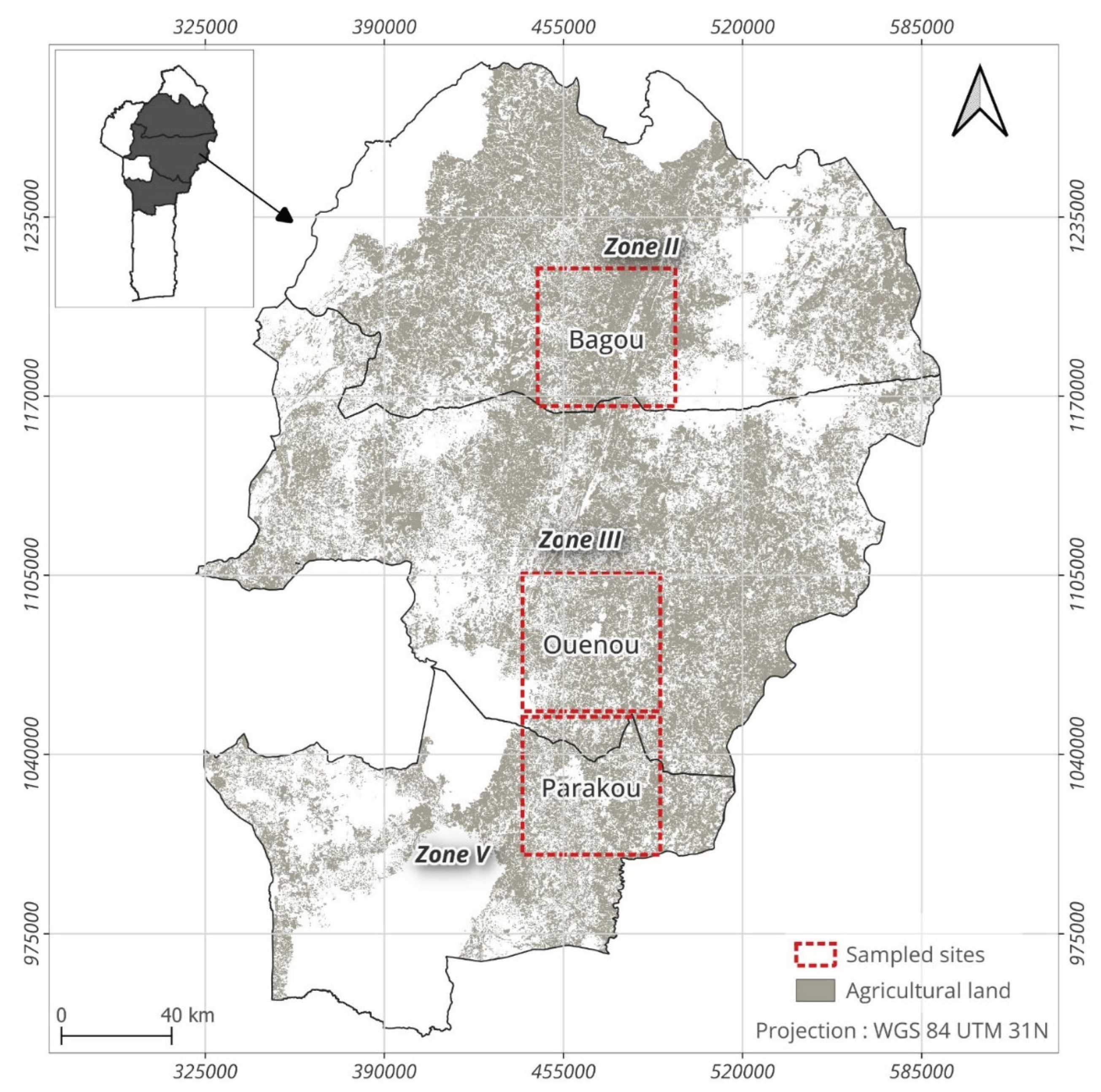
Figure 2.
Types of land cover in the three study sites
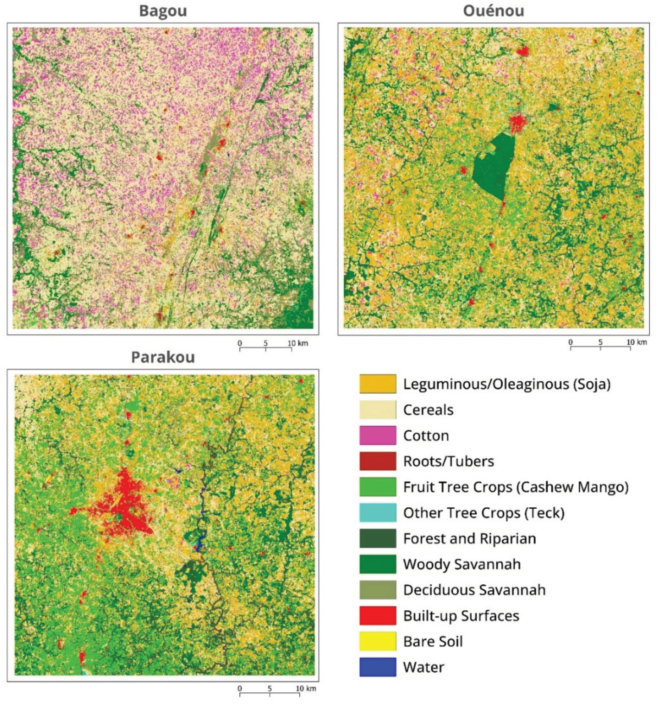
Figure 3.
Methodological framework for computing the Landscape Environmental Sustainability Index (LESI) for each study site (illustrated with the Bagou site), derived from 12-class land cover maps and 9 weighted criteria representing land cover-related negative externalities. The HDC and LESI are defined in Equations 1 and 2, respectively.
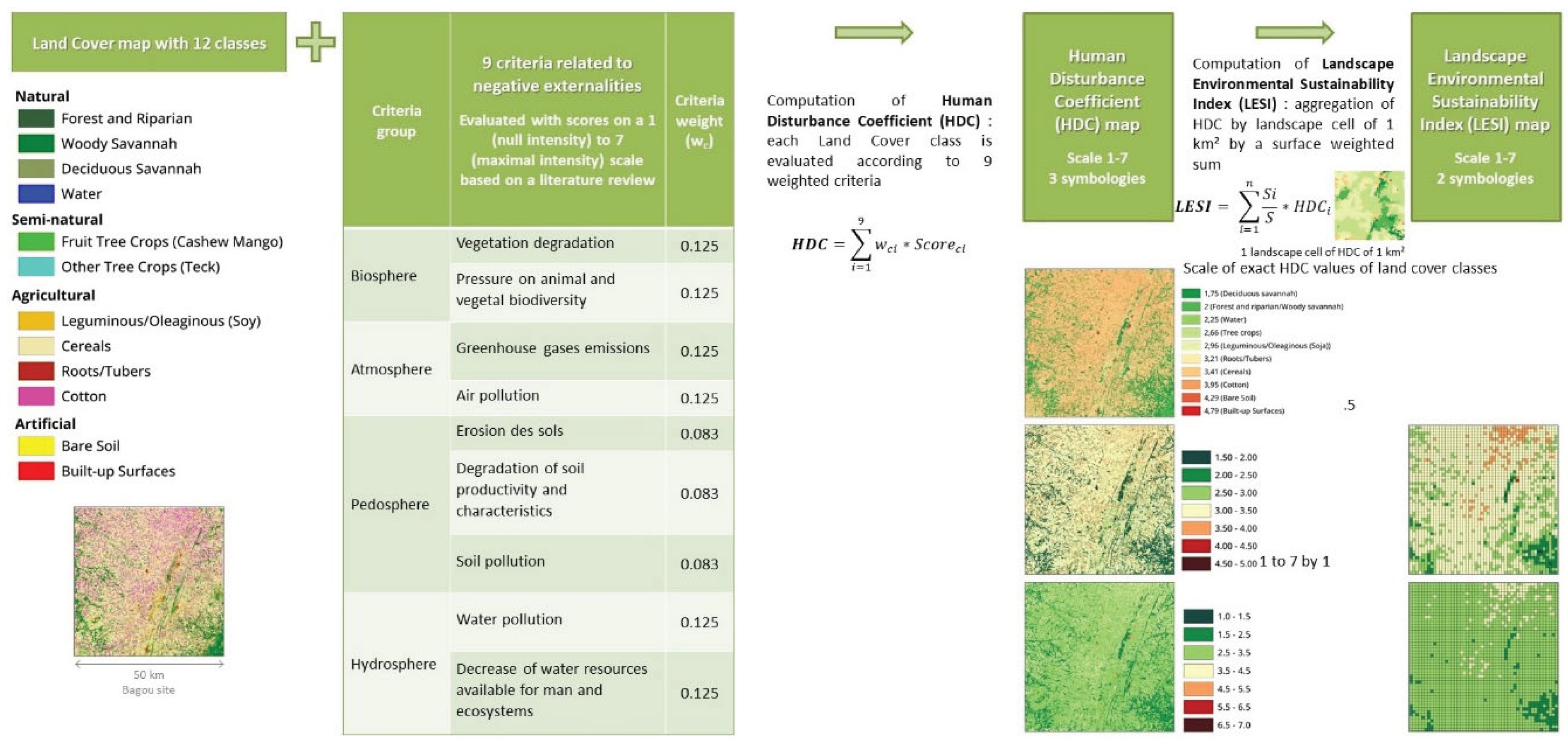
Figure 4.
Spatial variation of Human Disturbance Coefficient (HDC) by site
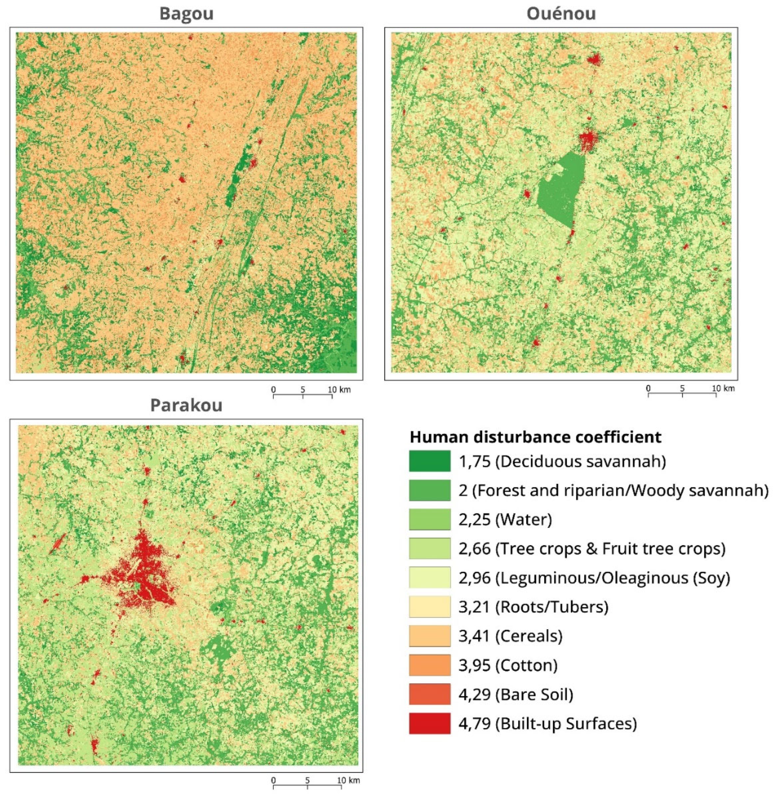
Figure 5.
Surface proportion by sites of (a) each unique Human Disturbance Coefficient (HDC) values encountered in this study, (b) regular classes of HDC values (with increment of 1), and (c) regular classes of LESI values (with increment of 1).
Figure 5.
Surface proportion by sites of (a) each unique Human Disturbance Coefficient (HDC) values encountered in this study, (b) regular classes of HDC values (with increment of 1), and (c) regular classes of LESI values (with increment of 1).
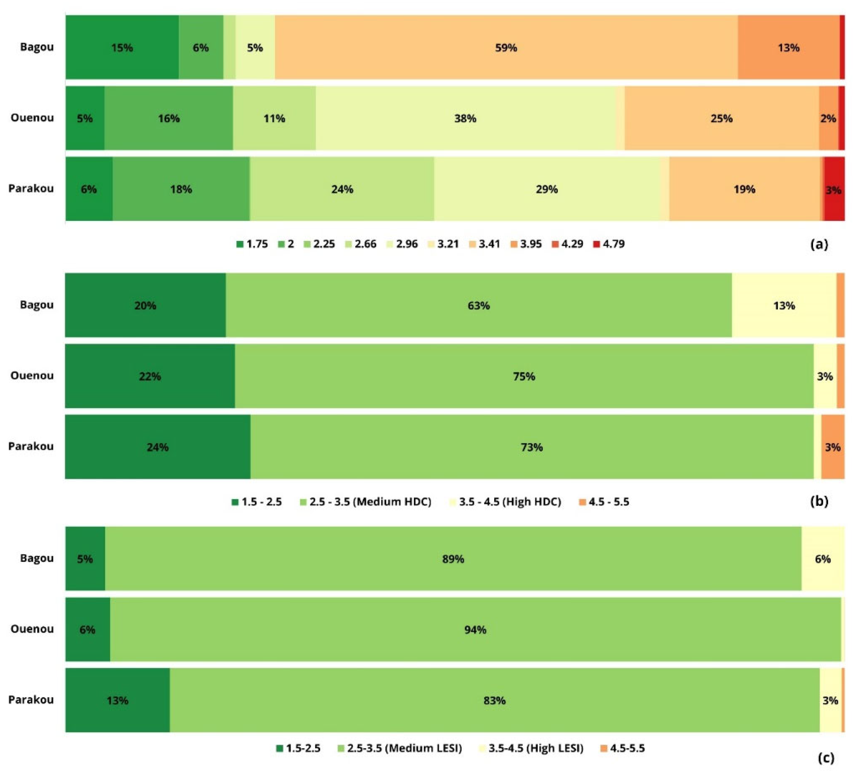
Figure 6.
Variation in Human Disturbance Coefficient (HDC) and Landscape Environmental Sustainability Index (LESI) by site with a color legend corresponding to (a) the theoretical range of values of these indicators, going from 1 to 7, with a unit increment, and (b) the range of values of these indicators effectively encountered in the study area (from 1.75 to 4.79) with a half unit increment.
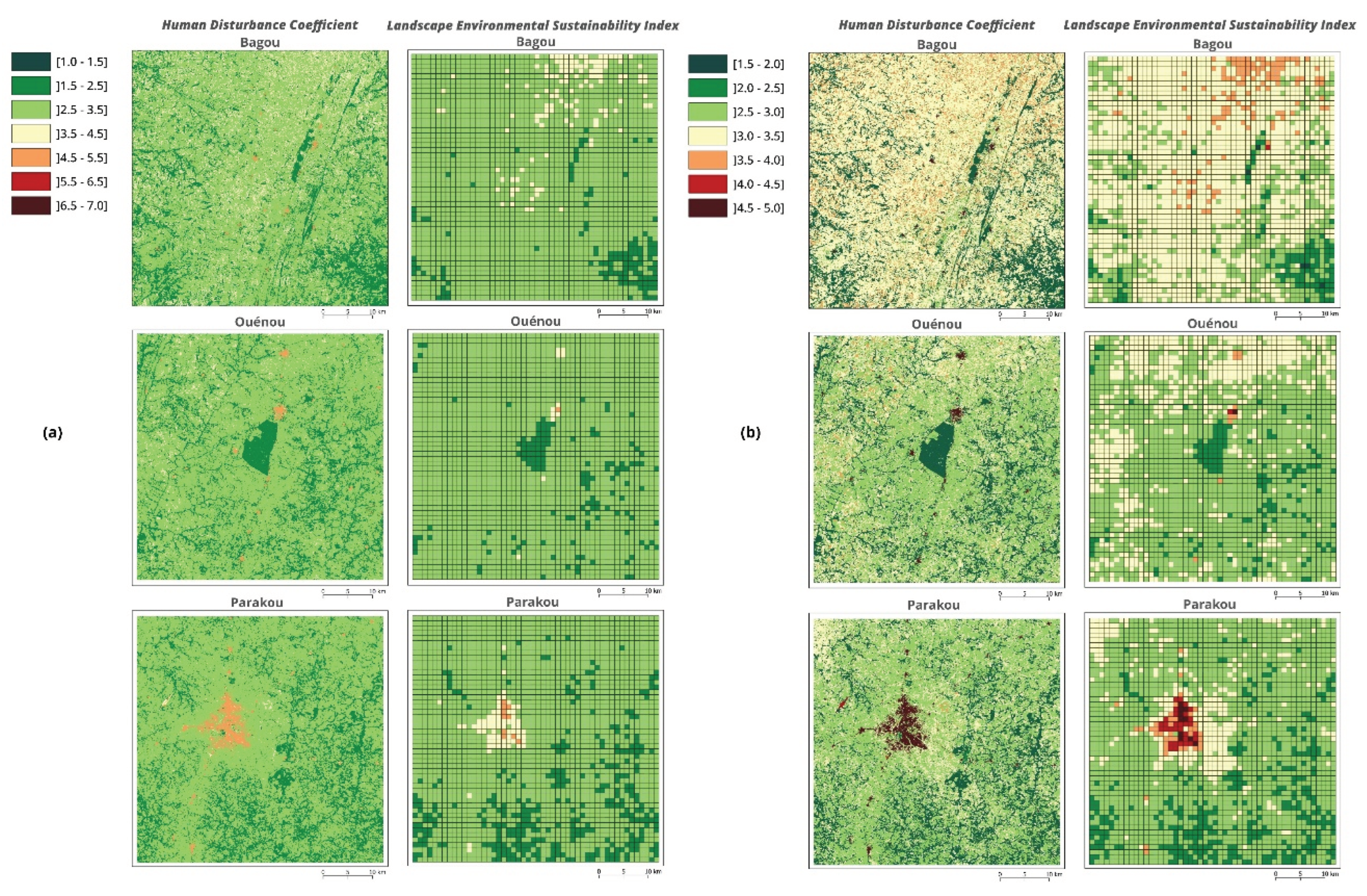

Table 1.
Description of remote sensing images used for the production of the land cover maps used in this study
Table 1.
Description of remote sensing images used for the production of the land cover maps used in this study
| Data type | Spatial resolution (m) | Collection time |
|---|---|---|
| SPOT 6/7 | 1.5 m | 21 and 27 October 2022 |
| Sentinel-2 | 10 m | Time series from 01/01/2022 to 31/12/2022 |
| SRTM | 30 m | 2000 |
Table 2.
Surface area (km²) and proportional coverage (%) of each land cover type across the three study sites.
Table 2.
Surface area (km²) and proportional coverage (%) of each land cover type across the three study sites.
| Land cover type | Bagou | Ouenou | Parakou | |||
|---|---|---|---|---|---|---|
| (km²) | (%) | (km²) | (%) | (km²) | (%) | |
| Forest and Riparian | 3,95 | 0,16 | 22,99 | 0,92 | 113,25 | 4,53 |
| Woody Savannah | 138,88 | 5,55 | 388,67 | 15,53 | 325,57 | 13,01 |
| Deciduous Savannah | 364,28 | 14,56 | 126,48 | 5,06 | 152,08 | 6,08 |
| Water | 0,78 | 0,03 | 0,13 | 0,01 | 3,93 | 0,16 |
| Other Tree Crops (Teck) | 13,33 | 0,53 | 26,91 | 1,08 | 27,12 | 1,08 |
| Fruit Tree Crops (Cashew, Mango) | 24,96 | 1,00 | 238,08 | 9,52 | 562,20 | 22,47 |
| Leguminous/Oleaginous (Soja) | 126,24 | 5,05 | 961,98 | 38,45 | 724,37 | 28,95 |
| Cereals | 1485,99 | 59,41 | 623,15 | 24,91 | 483,62 | 19,33 |
| Roots/Tubers | 0,03 | 0,001 | 30,47 | 1,20 | 29,97 | 1,20 |
| Cotton | 326,30 | 13,05 | 61,60 | 2,46 | 8,31 | 0,33 |
| Bare Soil | 1,06 | 0,04 | 2,97 | 0,12 | 6,62 | 0,26 |
| Built-up Surfaces | 15,56 | 0,62 | 18,50 | 0,74 | 64,93 | 2,60 |
| Total | 2501,36 | 100 | 2501,93 | 100 | 2501,97 | 100 |
Table 3.
Analysis criteria and scores description.
| Criteria | Score 1 (No intensity) |
Score 3 (Moderate) |
Score 5 (High) |
Score 7 (Maximum) |
|---|---|---|---|---|
| Degradation of vegetation | No degradation of the initial natural vegetation | Replacement of the original natural vegetation by tree plantations | Replacement of the original natural vegetation by intensive crops | Total disappearance of all forms of vegetation |
| Pressures on biodiversity | No pressure | Moderate intensity of the various pressures on biodiversity | High intensity of the various pressures on biodiversity | Total disappearance of all forms of animal and plant life |
| Greenhouse gas emissions | No emissions | Comparable to intensive agriculture | Comparable to that of an urban area with more than 10,000 inhabitants / km² | Comparable to an industrial zone using thermal energy |
| Air pollution | No pollution | |||
| Soil erosion | No erosion | Sheet erosion | Sheet and rill erosion | Sheet, rill and gully erosion |
| Degradation of soil productivity and characteristics | No degradation | Soil with a reduction in organic matter, loose, and with diversified plant cover | Soil devoid of organic matter, moderately compact, with little plant cover | Soil devoid of organic matter, compact, with no plant cover |
| Soil pollution | No pollution | Moderate-intensity pollution linked to urban or low-intensity agricultural activity | High-intensity pollution linked to intensive urban or agricultural activity | Extremely intense pollution linked to industrial discharges |
| Water pollution | No pollution | |||
| Reduction of water resources | No reduction in the water resources available to humans and ecosystems | Moderately problematic reduction in water resources available to humans and ecosystems | Highly problematic reduction in water resources available to humans and ecosystems | Extremely problematic reduction in water resources available to humans and ecosystems |
Table 4.
Weight of the 9 criteria used to compute the human disturbance coefficient and associated environmental systems.
Table 4.
Weight of the 9 criteria used to compute the human disturbance coefficient and associated environmental systems.
| Environmental systems | Land cover type | Criteria weights |
|---|---|---|
| Hydrosphere | Water pollution | 0.125 |
| Reduction of water resources | 0.125 | |
| Pedosphere | Soil pollution | 0.083 |
| Soil erosion | 0.083 | |
| Degradation of soil productivity | 0.083 | |
| Atmosphere | Air pollution | 0.125 |
| Greenhouse gases emissions | 0.125 | |
| Biosphere | Vegetation degradation | 0.125 |
| Pressures on biodiversity | 0.125 |
Table 5.
Criteria scores (as defined in Table 3) by land cover class and Human Disturbance Coefficients (HDC) resulting from the weighed sums of the scores. A score of 1 corresponds to no impact related to this criteria and a score of 7 corresponds to an impact of maximal intensity related to this criteria.
| Criteria | Weight | FR | WS | DS | WA | TC | FTC | LO | CER | RT | COT | BS | BUS |
|---|---|---|---|---|---|---|---|---|---|---|---|---|---|
| Degradation of vegetation | 0,125 | 2 | 2 | 2 | 1 | 3 | 3 | 4 | 4 | 4 | 5 | 6 | 6 |
| Pressures on biodiversity | 0,125 | 3 | 3 | 3 | 4 | 5 | 5 | 5 | 5 | 5 | 5 | 6 | 6 |
| Greenhouse gas emissions | 0,125 | 3 | 3 | 2 | 2 | 2 | 2 | 2 | 3 | 3 | 3 | 2 | 4 |
| Air pollution | 0,125 | 3 | 3 | 2 | 2 | 2 | 2 | 2 | 3 | 3 | 3 | 2 | 4 |
| Soil erosion | 0,083 | 1 | 1 | 1 | 1 | 3 | 3 | 4 | 4 | 4 | 4 | 6 | 6 |
| Degradation of soil productivity and characteristics | 0,083 | 1 | 1 | 1 | 1 | 3 | 3 | 4 | 4 | 4 | 4 | 6 | 6 |
| Soil pollution | 0,083 | 1 | 1 | 1 | 4 | 2 | 2 | 2 | 3 | 2 | 5 | 5 | 5 |
| Water pollution | 0,125 | 1 | 1 | 1 | 4 | 2 | 2 | 2 | 3 | 2 | 5 | 5 | 5 |
| Reduction of water resources | 0,125 | 2 | 2 | 2 | 1 | 2 | 2 | 2 | 2 | 2 | 2 | 2 | 2 |
| Human Disturbance Coefficient (HDC) | 2,00 | 2,00 | 1,75 | 2,25 | 2,66 | 2,66 | 2,96 | 3,41 | 3,21 | 3,95 | 4,29 | 4,79 | |
FR: Forest and Riparian; WS : Woody Savannah ; DS : Deciduous Savannah ; WA : Water ; Fruit Tree Crops (Cashew Mango) ;TC : Other Tree Crops (Teck) ; FTC : LO : Leguminous/Oleaginous (Soja) ; CER : Cereals ; RT : Roots/Tubers ; COT : Cotton ; BS : Bare Soil ; BUS : Built-up Surfaces
Disclaimer/Publisher’s Note: The statements, opinions and data contained in all publications are solely those of the individual author(s) and contributor(s) and not of MDPI and/or the editor(s). MDPI and/or the editor(s) disclaim responsibility for any injury to people or property resulting from any ideas, methods, instructions or products referred to in the content. |
© 2025 by the authors. Licensee MDPI, Basel, Switzerland. This article is an open access article distributed under the terms and conditions of the Creative Commons Attribution (CC BY) license (http://creativecommons.org/licenses/by/4.0/).
Copyright: This open access article is published under a Creative Commons CC BY 4.0 license, which permit the free download, distribution, and reuse, provided that the author and preprint are cited in any reuse.


