Submitted:
06 May 2025
Posted:
08 May 2025
You are already at the latest version
Abstract
Strategies to interpret short-wave infrared hyperspectral images of rocks involve the application of analysis and classification steps that guide the extraction of geological and mineralogical information with the ultimate aim of creating mineral maps. Previous interpretation strategies often rely on the use of statistical measures between reference and image spectra, which are scene dependent. Therefore, classification thresholds based on statistical measures to create mineral maps are also scene dependent, which is problematic because thresholds have to be adjusted between images to produce mineral maps of the same accuracy. We developed an innovative, knowledge-based interpretation strategy to perform mineralogical analyses and create classifications that overcome this limitation by using physics-based wavelength positions of absorption features, which are invariant between scenes, as the main sources of mineral information. The interpretation strategy is implemented using the open source Hyperspectral Python package (HypPy) and demonstrated on a series of laboratory-acquired hyperspectral images of hydrothermally altered rock samples. The results show how expert knowledge can be embedded into a standardized processing chain to develop reproducible mineral maps without relying on statistical matching criteria.
Keywords:
Shortwave Infrared
; Hyperspectal Imaging
; mineral analysis
; interpretation strategy
; Python
; mineral mapping
; proximal sensing
1. Introduction
Laboratory-based infrared hyperspectral imaging is a fast and non-destructive method to obtain mineralogical information from rock samples collected in the field [1,2,3,4,5,6]. Hyperspectral images provide spatially continuous mineralogical coverage of imaged rock surfaces and can be processed into mineral maps. The continuous coverage allows for the evaluation of spatial patterns and textures that emerge as a result of varying mineralogical composition in hyperspectral images. The level of mineralogical detail that can be derived from an image depends on many factors, including the spatial resolution of the image, the spectral resolution of the camera, and the wavelength range imaged [7]. The wavelength range imaged by the camera determines which minerals can be mapped since the wavelength position of diagnostic absorption features varies between minerals [8,9].
Numerous methods have been developed for the interpretation and extraction of mineralogical information from hyperspectral images (e.g., [10,11,12]). Interpretation strategies are defined as the series of steps performed to extract mineralogical information from hyperspectral images by the application of specific analysis, classification and/or mapping methods. An example of such a strategy is the commonly used ENVI1 hourglass approach [13,14]. This approach involves i) the identification of mineralogical endmembers (i.e., unique spectra of minerals present in the image), ii) the matching of these endmember spectra to each of the image pixel spectra using statistical measures, iii) the definition of thresholds that reflect positive matches to the various endmembers, and iv) the classification of pixels using the defined thresholds in a mineral map of the identified endmembers. Many commonly used methods for matching endmember spectra to image-pixel spectra for mapping of mineralogical composition include the Spectral Angle Mapper (SAM) [15], Mixture Tuned Matched Filtering [16], and Linear Spectral Unmixing [17] and, more recent, machine learning algorithms [18].
Interpretation strategies that rely on statistics-based algorithms to measure similarities between endmembers and image-pixel spectra to construct mineral maps have several weaknesses. First, the algorithms require the setting of threshold values to define matches between the reference and unknown spectra. The definition of thresholds is a subjective process because the values are influenced by the image characteristics, which depend on factors such as the specifications of camera used, the applied calibration procedures and minerals present in the rock (e.g., [19]. Therefore, the statistics-based thresholds for classifying pixel-spectra into minerals vary between measurement campaigns and between different rocks. This means that there are no universal statistical thresholds for the classification of hyperspectral images into mineral maps. The definition of thresholds requires systematic manual interference and is time consuming and therefore less suitable for the classification of a large number of images of multiple rocks and measured during different campaigns. Secondly, statistical matching algorithms, such as SAM, do not provide information on the specific wavelength range at which the endmember and the pixel spectrum match. The degree of matching is expressed as one value for the match over the entire wavelength interval. This means that it is impossible to know whether the match is the result of matching absorption features between the unknown and reference spectra, or similarity in the overall shape of the curve of the two reflectance spectra.
We present a novel strategy for the interpretation of hyperspectral images and the creation of mineral maps that does not depend on statistical relationships or statistical matching criteria. The strategy is knowledge-based and suitable for the interpretation of large hyperspectral image data sets of multiple rocks. The main characteristics are i) the incorporation of expert knowledge in the various steps in the workflow, ii) the focus on the analysis of physics-based wavelength positions of absorption features, iii) the evaluation of spatial patterns in wavelength images, summary products, and iv) the automation of parts of the processing and classification steps.
In this paper, we describe the strengths and weaknesses of the interpretation strategy using an example analysis of previously collected hydrothermally altered rocks that were imaged with a hyperspectral camera in the ShortWave InfraRed (SWIR) wavelength range at 26 m pixel size.
2. Materials and Methods
2.1. Interpretation Strategy
The strategy for the interpretation of SWIR hyperspectral images of rocks is presented in Figure 1. Step 1 involves the creation of wavelength maps, summary products, decision tree classifications and mean spectra of classes. The methods to create these products are described in Section 2.3, Section 2.4, Section 2.5 and Section 2.6, respectively. Step 2 involves the exploratory analysis of the images, maps and spectra, produced in step 1, to determine variation in spectral features, reflectance spectra and their spatial distribution in the hyperspectral images.
Step 3 involves a comparison of the images and spectra produced in step 1 with complementary mineralogical and chemical analyses, acquired by, for example, petrography and electron microprobe. The aim of this comparison is to identify the different minerals with their chemical variation and the interpretation of spatial patterns. In step 4 an improved classification scheme is developed that is specific to the imaged rock samples that are being studied, based on the exploratory analysis in step 2 and comparison with complementary data in step 3. The processing chain describes the processing and classification steps to create this improved classification and can be automated. The application of the processing chain in step 5 results in the creation of mineral maps.
2.2. Image Acquisition and Preprocessing
Hyperspectral images were acquired from slabs of the 11 rock samples (see Section 2.8) with a Specim SWIR camera (model SWIR 3, Serial number SN430024, date 12.11.2015) and OLES Macro lens mounted in a Sisuchema instrument setup (Specim, Spectral Imaging Ltd, Oulu, Finland) from 894 to 2511 nm in 288 bands at 26 m pixel size. Image sizes were 384 by approximately 1200 pixels, resulting in images of a width of 11 mm and a length of approximately 3 cm.
The raw images were converted to reflectance using dark current and white reference measurements acquired during the recording of the images. Noise reduction involved i) removal of bad pixels that produced anomalous pixel values, ii) the identification and removal of bad bands near the lower (1000 nm) and higher (2500 nm) margins of the measured wavelength range, and iii) application of a spatial-spectral smoothing filter that averaged five spatial and two spectral neighboring pixel values [20]. The filter was applied to reduce noise in the pixel spectra by a factor 7 approximately. Care was taken to ensure that shallow absorption features were not filtered out by the spectral smoothing process. The noise-reduced images are available at [21].
2.3. Wavelength Mapping
Wavelength images and maps were created from the noise-reduced reflectance images. The wavelength mapping method has been described in various papers (e.g., [22,23]). The method was performed in two steps. First, a wavelength image was calculated that contains the wavelength positions and depths of absorption features in each pixel spectrum. After that a wavelength map was created by displaying the wavelength position in color and the feature depth in gray scale in the same map. For the calculation of the wavelength images, the continuum was removed by division to negate the effect of albedo differences between image pixels. Wavelength images were calculated over wavelength ranges of 1300-1600 nm, 1650-1850 nm, 1850-2100 nm, and 2100-2400 nm. Three deepest features were calculated for each wavelength range. The values of wavelength positions and depths of absorption features were analysed in scatterplots (for example Figure 7), and as color composite images of the wavelength positions of the three deepest wavelength positions in red, green, and blue, respectively (for example Figure 4a). Wavelength maps were created from the wavelength images with stretching intervals of 1300-1600 nm, 1650-1850 nm, 1850-2100 nm, 2100-2400 nm and 2185-2225 nm (for example Figure 3c&d). These wavelength ranges contain complementary information on specific molecular bonds, e.g., in OH, H2O, AlOH, FeOH, MgOH, SiOH and in lattices of the minerals present in the rocks (see for instance [9] for an overview of wavelength ranges of mineral absorption features). The wavelength maps provided intuitively interpretable visualisations of wavelength positions and depths of mineral absorption features in rock.
2.4. Summary products
Summary products are defined here as images that result from mathematical operations on image bands or spectra to indicate specific minerals or parameters (e.g., [24]). The summary products albedo, ferrous drop, illite-kaolinite and Shannon entropy (Table 1) were calculated from the noise-reduced reflectance. The summary product illite crystallinity (Table 1) was calculated from absorption feature depths in wavelength images between 1850-2100 nm and 2100-2400 nm.
2.5. Decision trees
Decision trees were applied to convert the wavelength images into classified images and to slice all summary products into classes according to predefined, generically applicable thresholds. Decision trees consist of a series of binary nodes with Boolean statements that are true or false [28]. An example of such a Boolean statement is ”the wavelength position of the deepest feature is between 2190 and 2200 nm.” This statement is either true or false depending on the values in the wavelength image. By connecting multiple binary nodes, a decision tree is formed that classifies all pixels based on the expressions in the nodes. A major advantage of the classification of wavelength images and summary products using invariant thresholds in the decision trees is that the resulting images contain the same sets of classes between images, which makes the classes comparable between images and across different acquisitions.
The decision trees in this study were built using experience with the interpretation of mineral reflectance spectra, which includes knowledge of the wavelength positions and depths of absorption features in the spectra and the range of values of summary products calculated from the spectra. The decision trees , , , and (Table 2) were created for the exploratory analysis and comparison with other mineral and chemical analyses in steps 2 and 3 in Figure 1.
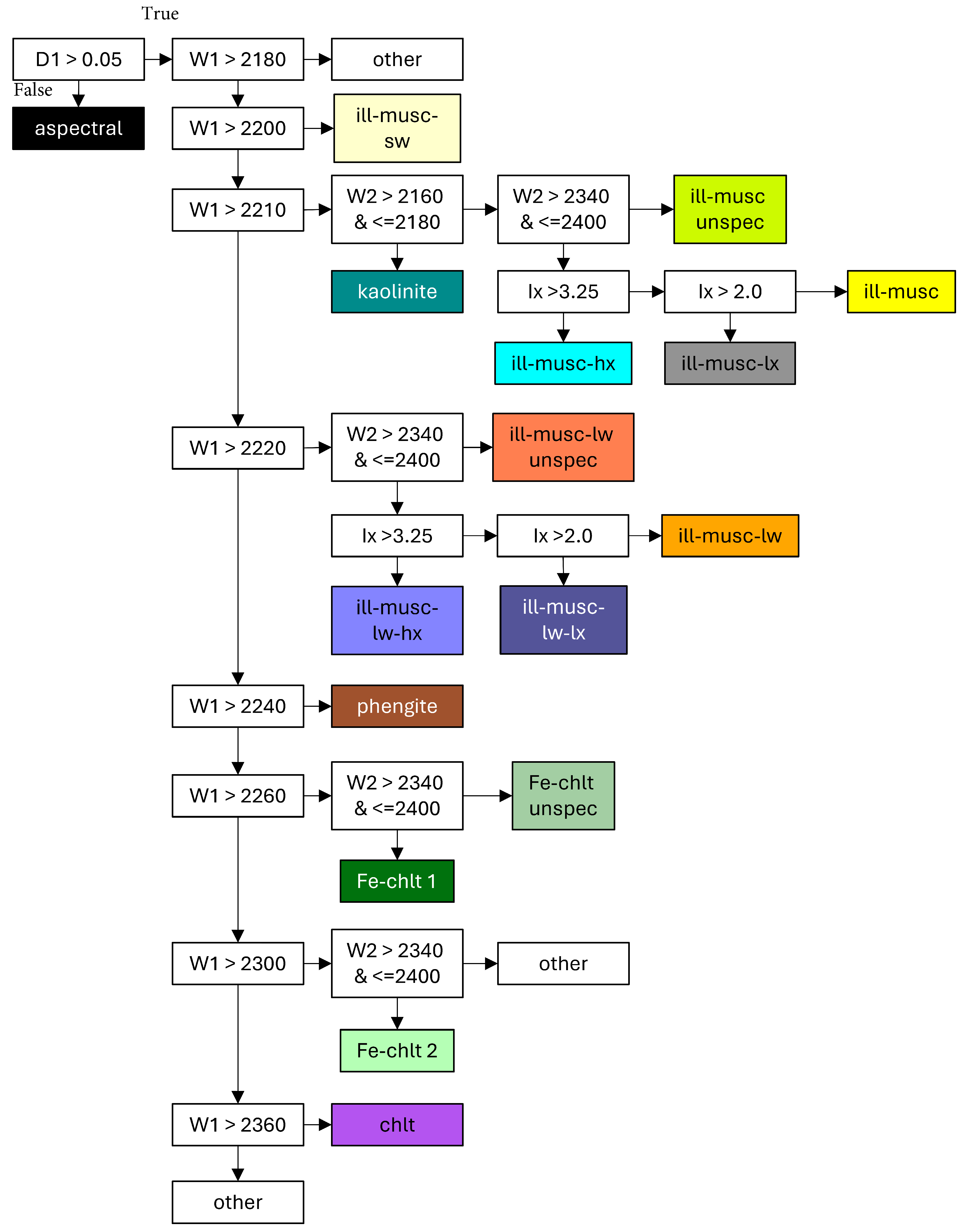
Decision tree (Table 2, Figure 2) resulted from the improved classification scheme in step 4 and was applied in the processing chain in step 5 to create mineral maps (Figure 1). The depth and wavelength position of absorption features between 2100 and 2400 nm and illite crystallinity were used for the classification. The decision tree classifies the images into ilite-muscovite minerals of different composition and crystallinity, kaolinite and different types of chlorite. The application of this tree involves i) selection of pixels with a minimum feature depth of 0.05 reflectance in the rectangular box at the upper left of the decision tree in Figure 2 (pixels with shallower depth end up in the box below are named "aspectral"), ii) subdivision of pixels with absorption feature larger than 5% along right-hand branches of the three of the wavelength of deepest absorption features (W1) at 2180 nm, 2200 nm, 2210 nm, 2220 nm, 2240 nm, 2260 nm, 2300 nm, and 2360 nm (along the second column in Figure 2), and iii) further subdivision of the pixels by slicing the wavelength positions of second deepest absorption features (W2) at 2160 nm, 2180 nm, 2340 nm, and and 2400 nm, and crystallinity values (Ix) at 2 and 3.25, along the third to sixth column. In the resulting classification, all image pixels are assigned to one of the classes in the decision tree and labeled accordingly. Classes that were labelled ”other” were not present in the rock sample set or they were present in very small quantities.
The decision trees were also applied to reference spectra from spectral libraries to test the performance of decision trees and to verify if the classifications produced the required results (see example in Figure Table 4).

Table 2.
Description of decision trees to classify wavelength images (Section 2.3) and summary products in Table 1. See Figure 2 and Appendix C for the design of the decision trees. Thresholds for slicing and classification are based on experience with the interpretation of mineral spectra.
Table 2.
Description of decision trees to classify wavelength images (Section 2.3) and summary products in Table 1. See Figure 2 and Appendix C for the design of the decision trees. Thresholds for slicing and classification are based on experience with the interpretation of mineral spectra.
| Decision tree | Resulting classified image | Description |
|---|---|---|
| wave2100-2400_class | Classification based on depth of deepest and wavelength positions of first and second deepest absorption features in wavelength image between 2100 and 2400 nm (see Figure A2). | |
| albedo_class | Slicing of albedo image at thresholds: 0.25, 0.38 and 0.50 (see Figure A3). | |
| fedrop_class | Slicing of ferrous drop (fedrop) image at thresholds: 1.1, 1.2, 1.3, 1.4 and 1.5 (see Figure A4). | |
| illx_class | Slicing of illite crystallinity (illx) image at thresholds: 0.25, 0.33, 0.5, 1, 2, 3 and 4 (see Figure A5). | |
| illkaol_class | Slicing of illite over kaolinite (illkaol) image at thresholds: 0.95, 0.97, 0.99, 1.0, 1.01, 1.03 and 1.05 (see Figure A6). | |
| mineral_map | Classification using depth and wavelength positions of deepest features in the wavelength images between 2100 and 2400 nm and the illite crystallinity image. Customized for the rock sample set in this study (see Figure 2). |
Figure 2.
Design of decision tree (Table 2) developed in step 4 (Figure 1) for the classification of the hyperspectral images of the eleven rock samples in this study. Input bands are depth of deepest absorption feature between 2100 and 2400 nm (D1) and wavelength position of deepest (W1) and second deepest (W2) features and illite crystallinity (Ix). Vertical arrows present a "false" to the binary statements, horizontal arrows present a "true". The class "other" represents classes that did not occur in the rock sample set or occurred in very small quantities. ill=illite, musc=muscovite, chlt=chlorite, unspec=unspecified, lx=low crystallinity, hx=high crystallinity, lw=long wavelength, sw=short wavelength.
2.6. Mean Spectra of Classes
For each class in the classified images, the mean reflectance spectrum for that class was calculated, as well as the number of pixels in that class. The mean spectra were used in the exploratory analysis, the comparison with other chemical and mineral analyses, and the development of the improved classification scheme (steps 2, 3 and 4 of Figure 1) to interpret the mineralogy of the class from which it was derived. The percentage of pixels per class was useful for quantifying the mineralogical composition and for filtering out small classes. Small classes may represent noise (shown, for instance, by erroneous pixel spectra) or mineral variations that are not of interest. They can be removed from the analysis or merged with other classes, respectively. Care must be taken not to remove small, but geologically significant, classes.
2.7. HypPy Software
The processing and classification steps in the interpretation strategy run entirely on routines in the Hyperspectral Python (HypPy) software. HypPy is open source software and can be operated with a GUI and from the command line in both GNU/Linux and Windows environments [20]. The creation of images and spectra in step 1 and the application of the processing chain in step 5 to create the "final" mineral maps (Figure 1) were automated using HypPy software. Automation was achieved by executing command line statements of HypPy (see Appendix A) in a series of GNU/Linux shell scripts.
2.8. Test Sample Set and Validation
The test sample set consists of eleven rock samples collected from hydrothermally altered sections of the Archean Soanesville greenstone belt in the Pilbara craton in Australia. The samples were collected along a transect crosscutting different alteration zones showing a variety of minerals and micro structures. The rock sample set was selected because the rocks contain a diversity of SWIR active minerals of varying chemical composition (detectable as minor shifts in wavelength positions of absorption features), hull shapes and overlapping features, that are challenging to differentiate using statistics-based mapping methods. Furthermore, the petrography, mineralogy and chemistry of the rock samples have been analyzed and described in detail by [29] and [30]. Ten of the rocks are hydrothermally altered volcanics of andesitic to basaltic composition (see Table 3). The availability of detailed chemical and mineral analyses allowed for the comparison and validation of the mineral maps produced from the hyperspectral images. Three of those are chlorite-quartz altered and six are white mica altered. The white mica altered rocks are divided in two groups, one contains relatively Al-rich white mica, which is apparent from the relatively short wavelength position of the 2200 nm absorption feature. The other group is relatively Al-poor and has a longer wavelength position of the 2200 nm feature. One of the rock samples contains kaolinite, likely the result of weathering. One sample represents a silicified sediment (chert).
The results of the exploratory analysis of the hyperspectral data and the comparison with the petrographic, chemical and mineralogical data of the eleven rock samples are presented in subSection 3.1 Exploratory analysis. The mineral map that resulted from the comparison is presented in subSection 3.2 Mineral maps.
Table 3.
Geological characteristics of samples used in this study determined by petrography, whole rock geochemistry, microprobe and field spectrometer analysis [29,30].
| ID | Sample | Description |
|---|---|---|
| 1 | P2003 | Weakly sericite altered and silicified muddy chert. |
| 2 | P2004 | Deuterically altered, silicified, seriticized (Al-rich), xenocrystic phenocrystic andesite. |
| 3 | P2005 | Deuterically altered, silicified, seriticized (Al-rich), phenocrystic andesite. |
| 4 | P2006 | Deuterically altered, silicified, seriticized (Al-rich), weakly phenocrystic andesite. |
| 5 | P2007 | Deuterically altered, silicified, seriticized (Al-rich), weakly phenocrystic quenched andesite. |
| 6 | P2008 | Deuterically altered, silicified, seriticized (Al-poor), weakly phenocrystic andesite. |
| 7 | P2009a | Deuterically altered, silicified, seriticized (Al-poor), weakly xenocrystic amygdaloidal basalt. Contains aproximately 15% kaolinite in amygdales. |
| 8 | P2010 | Deuterically altered, silicified, seriticized (Al-poor), weakly xenocrystic weakly amygdaloidal basalt. |
| 9 | P2012 | Deuterically altered, silicified, ferruginous, chloritised basalt. |
| 10 | P2013 | Deuterically altered, silicified, ferruginous, chloritised (pyroxene-bearing) basalt. |
| 11 | P2014 | Deuterically altered, silicified, chloritised amygdaloidal andesite. |
3. Results
3.1. Exploratory Analysis
Selected wavelength maps, summary products and classifications of the 11 rock samples created in step 1 of the interpretation strategy (Figure 1) are shown in Figure 3, Figure 4 and Figure 5. Wavelength maps calculated from other wavelength ranges are presented in Appendix B.
The albedo images in Figure 3a show the brightness of the different rocks in shades of grey. These images show rock microstructures, such as layering, phenocrysts and amygdales, as well as artificial surface features such as saw marks. Differences in brightness in the images is enhanced by linear stretching (+/- 2 standard deviations) of the image according to the image-specific pixel values. The brightness differences between the rocks can be observed in the multi-level thresholded albedo image in Figure 3b by applying the same thresholds between images. The sliced albedo images show that the quartz-sericite altered rocks 2 to 8 are brighter than rock 1 (a chert) and the chlorite-quartz altered rocks 9 to 11.
Wavelength maps between 2100 and 2400 nm show that the wavelength position of deepest absorption features near 2205 nm and 2350 nm (green and yellow colors, respectively in Figure 3c.) are the most abundant, and that the 2205 nm feature dominates over the 2350 nm feature because of the more abundant green colors. The wavelength map in Figure 3d shows the result of the calculation of the wavelength image between 2100 and 2400 nm and subsequent mapping over the range between 2185 and 2225 nm to create the wavelength map. These maps shows the contrast in the wavelength position of absorption features near 2205 nm in green, red, orange and yellow colors. The green colors indicate white micas of relatively short wavelength position between 2200 and 2205 nm (rocks 2-4), the orange-red colors indicate a shift of the Al-OH absorption feature to longer wavelengths up to approximately 2215 nm (rocks 5-9).
Figure 3.
Wavelength maps, summary products and classifications of the hyperspectral images of the eleven rock samples: (a) Albedo, (b) classified albedo image (albedo_class), (c) wavelength map between 2100-2400 nm, (d) wavelength map between 2100-2400 nm and stretched between 2185-2225 nm. See Table 2 for decision trees used for classification. Rock samples: 1=P2003, 2=P2004, 3=P2005, 4=P2006, 5=P2007, 6=P2008, 7=P2009a, 8=P2010, 9=P2012, 10=P2013 and 11=P2014. See Table 3 for descriptions of the rock samples. Width of the images is 1.1 cm. med=medium.
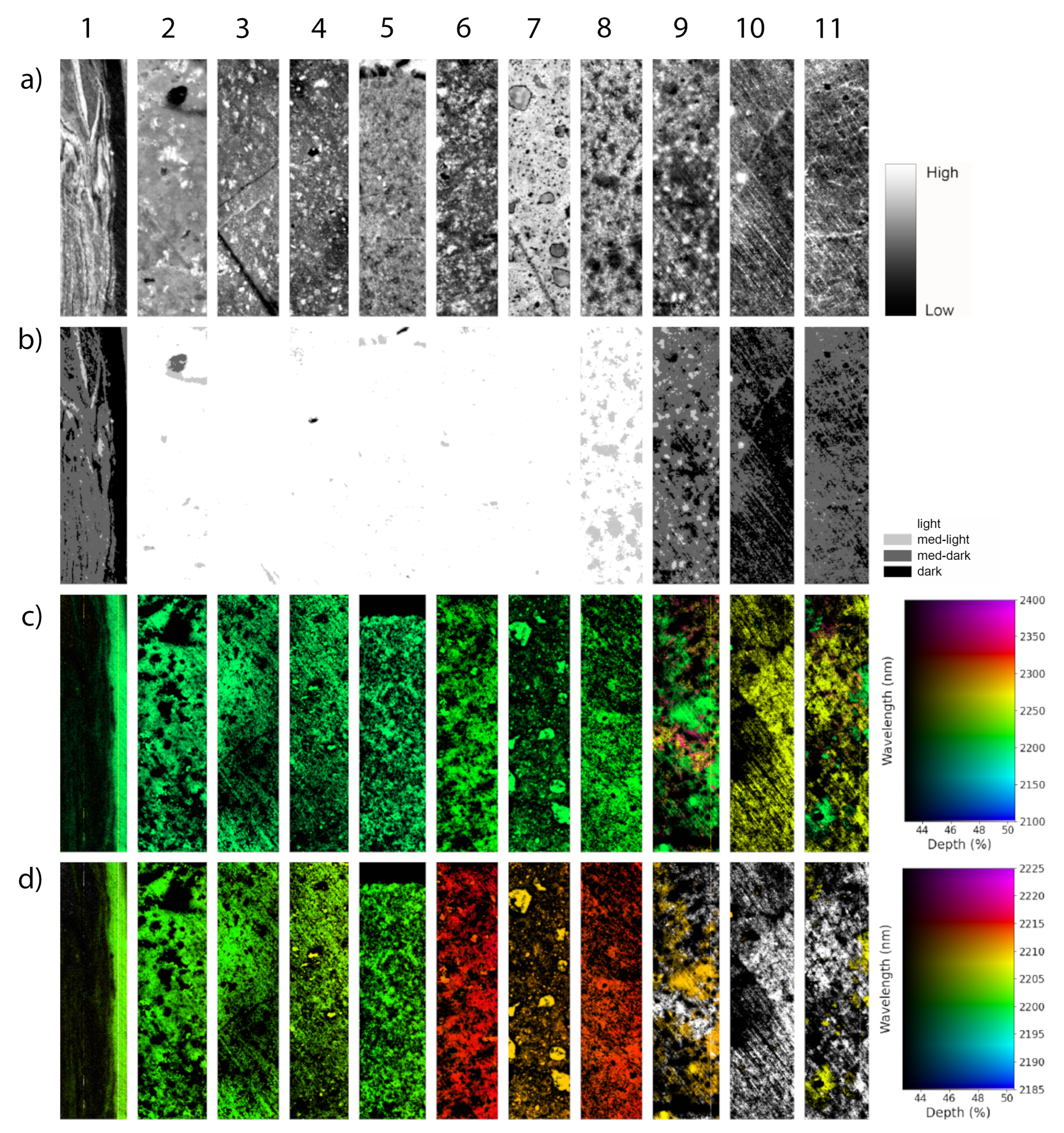
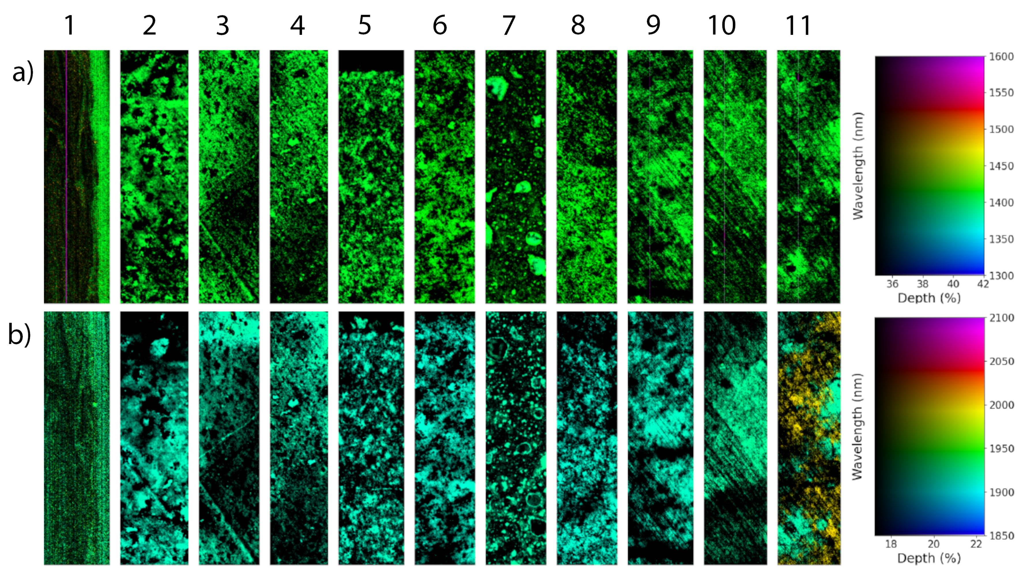
Figure 4.
Wavelength images, wavelength maps and classifications of the hyperspectral images of the eleven rock samples: (a) Color composite of wavelength positions of the first, second and third deepest absorption features, respectively w1, w2 and w3, between 2100-2400 nm, (b) classified wavelength image between 2100-2400 nm (wave2100-2400_class), (c) wavelength map between 1650-1850 nm, (d) classified fedrop image (fedrop_class). See Table 2 for decision trees used for classification. Rock samples: 1=P2003, 2=P2004, 3=P2005, 4=P2006, 5=P2007, 6=P2008, 7=P2009a, 8=P2010, 9=P2012, 10=P2013 and 11=P2014. See Table 3 for descriptions of the rock samples. Width of the images is 1.1 cm. ill=illite, musc=muscovite, kaol=kaolinite, chlt=chlorite, med=medium.
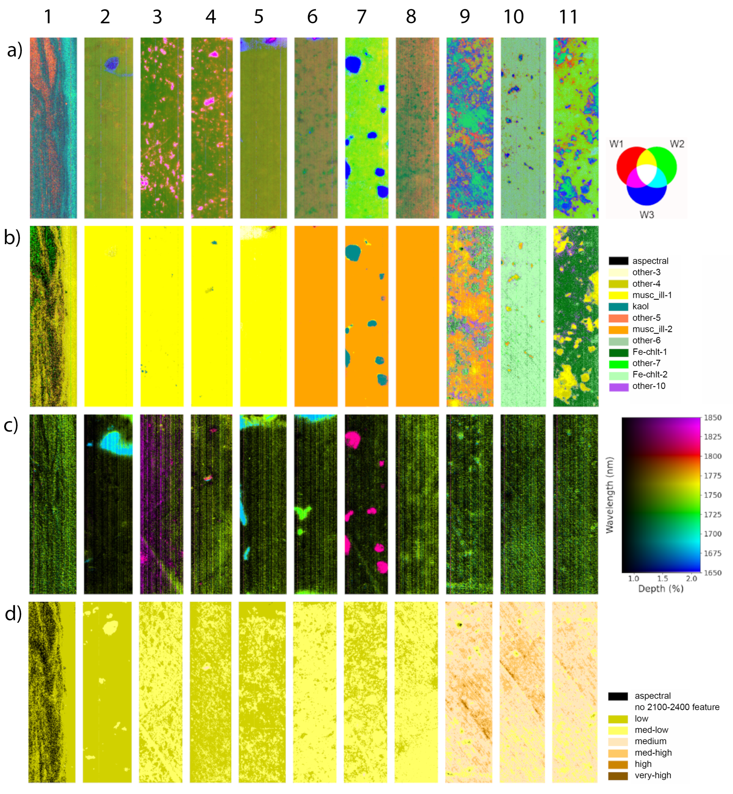
Figure 5.
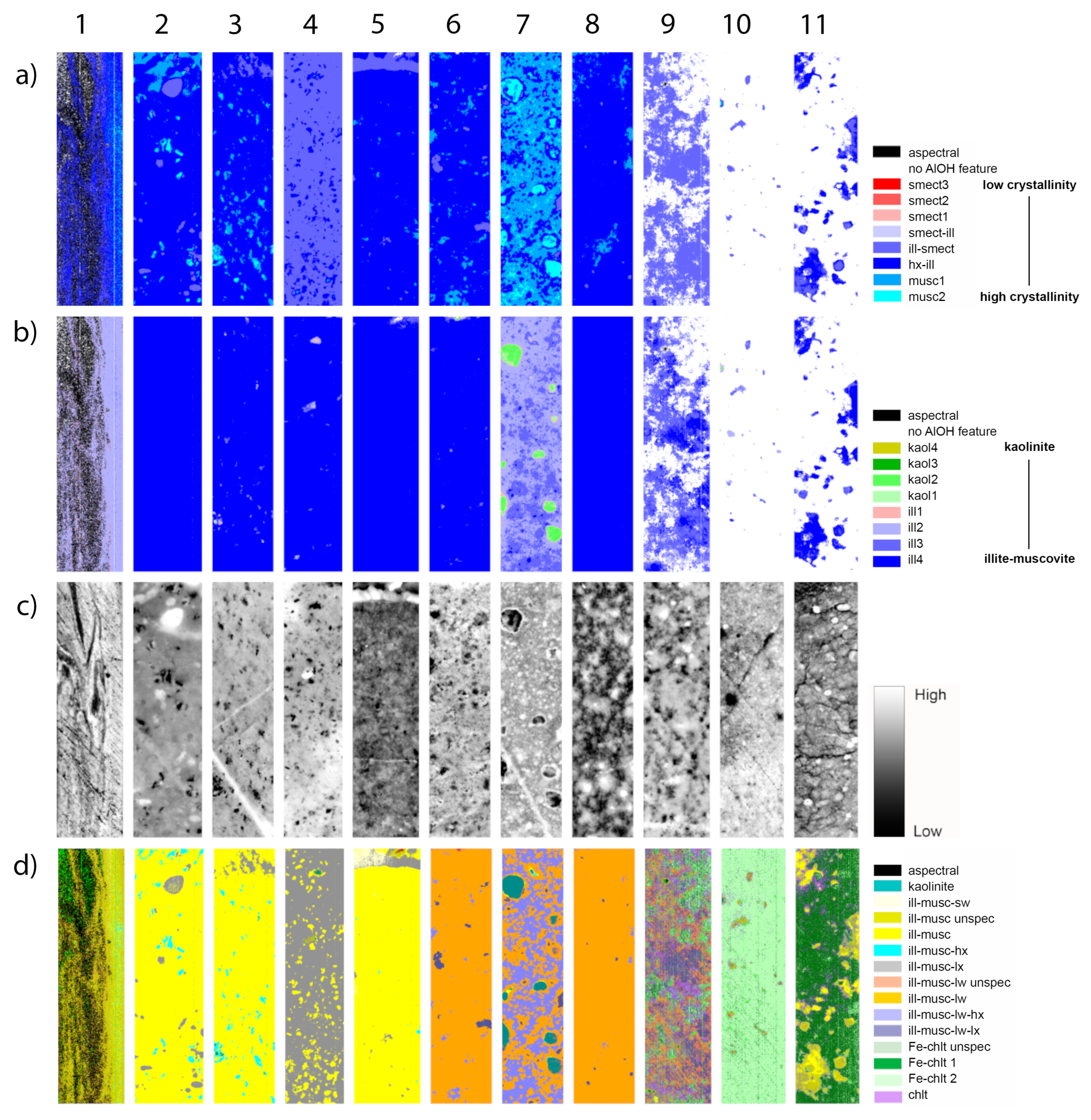
Summary products and classifications of the hyperspectral images of the eleven rock samples: (a) Classified illite crystallinity image (illx_class), (b) classified illite over kaolinite image (illkaol_class), (c) entropy, (d) mineral map (mineral_map). See Table 2 for decision trees used for classification. Rock samples: 1=P2003, 2=P2004, 3=P2005, 4=P2006, 5=P2007, 6=P2008, 7=P2009a, 8=P2010, 9=P2012, 10=P2013 and 11=P2014. See Table 3 for descriptions of the rock samples. Width of the images is 1.1 cm. smec=smectite, ill=illite, musc=muscovite, kaol=kaolinite, chlt=chlorite, unspec=unspecified, sw=short wavelenght, lw=long wavelength, lx=low crystallinity, hx=high crystallinity
Figure 5.
Summary products and classifications of the hyperspectral images of the eleven rock samples: (a) Classified illite crystallinity image (illx_class), (b) classified illite over kaolinite image (illkaol_class), (c) entropy, (d) mineral map (mineral_map). See Table 2 for decision trees used for classification. Rock samples: 1=P2003, 2=P2004, 3=P2005, 4=P2006, 5=P2007, 6=P2008, 7=P2009a, 8=P2010, 9=P2012, 10=P2013 and 11=P2014. See Table 3 for descriptions of the rock samples. Width of the images is 1.1 cm. smec=smectite, ill=illite, musc=muscovite, kaol=kaolinite, chlt=chlorite, unspec=unspecified, sw=short wavelenght, lw=long wavelength, lx=low crystallinity, hx=high crystallinity
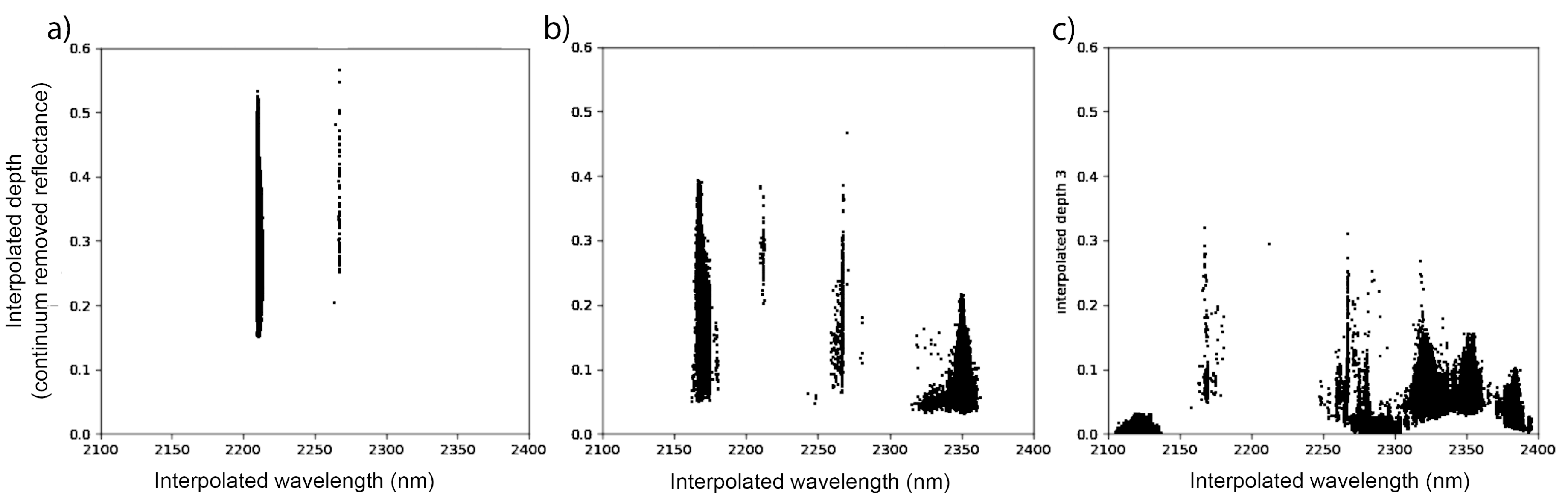
The variation in wavelength positions of the three deepest absorption features is highlighted in Figure 4a, which is a color composite of the wavelengths of first, second and third deepest features between 2100 and 2400 nm. The different colors indicate different combinations of wavelength positions of absorption features, which are largely the result of varying amounts and types of illite-muscovites, chlorites, kaolinite and their mixtures. Because each image is stretched according to its wavelength position statistics, similar minerals may show in different colors between images. Kaolinite in rock 7 of Figure 4a is shown in blue (R:∼2209 nm; G:∼2166 nm; B:∼2320 nm); white micas surrounding the kaolinite occurrences in the same rock are shown in yellow-green (R:∼2210 nm; G:∼2351 nm; B:∼2115 nm). The scatter plots in Figure 7 show the wavelength positions and the three deepest features for each pixel in the wavelength image of rock 7. The deepest features in Figure 7a are largely confined to a narrow cluster between 2209 and 2213 nm and 0.15 and 0.50 reflection. These values are consistent with deepest absorption features of kaolinite and white mica minerals. The wavelength positions of second deepest features in Figure 7b cluster near 2166 and 2350 nm, which is consistent with kaolinite and muscovite, respectively (see mean class spectra of kaolinite and illite-muscovite in Figure 6). Third deepest features cluster at various wavelengths and are generally shallower. The cluster at ∼2320 nm in Figure 7c represents kaolinite; the cluster near ∼2115 nm represents white micas. The blue kaolinite clusters in rock 7 Figure 4a represent amygdales in the volcanic rock found in the petrographic study of the rocks (Table 3). The magenta-colored pixels in Figure 4c show the 1820 nm feature of kaolinite (see kaolinite spectrum in Figure 6). The blue circular object near the top in rock 2 of images Figure 4a corresponds to a xenocryst in the volcanic rock. The maps in Figure 4b resulted from the classification of the wavelength images between 2100 and 2400 nm using the decision tree (Tab. Table 2). This decision tree classifies pixel-spectra by the wavelength position of the deepest and second deepest absorption features which are determined by the type and strength of the molecular bonds in Al-OH, Fe-OH, Mg-OH and carbonate molecules in mineral lattices. The maps in Figure 4b show two illite-muscovite dominant assemblages, one with relatively short wavelengths in yellow (rock samples 2, 3, 4 and 5) and a second with longer wavelengths in orange (rock samples 6, 7 and 8). The maps also show chlorite dominant assemblages in green (rock samples 10 and 11). Rock 9 contains mixtures of illite-muscovite and chlorite. The clusters of yellow pixels in rock 11 show white mica rich amygdales in the predominantly chlorite-altered rock. In white mica and chlorite mixtures, white micas often dominate the spectra, possibly because they are brighter than chlorites.
Figure 6.
Mean spectra of ten representative classes in the mineral maps in Figure 5d: One chert (p2003 aspectral), two chlorite-illite/muscovite mixtures (p2014 Fe-chlt1 and p2013 Fe-chlt2), one kaolinite (p2009a kaolinite) and seven illite/muscovite dominated spectra (p2004 ill-musc-hx, p2004 ill-musc-lx, p2004 ill-musc, p2008 ill-musc-lw-hx, p2008 ill-musc-lw-lx, and p2008 ill-musc-lw). The spectrum names refers to the sample number and mineral class from which the mean spectrum was obtained. ill=illite, musc=muscovite, kaol=kaolinite, chlt=chlorite, sw=short wavelenght, lw=long wavelength, lx=low crystallinity, hx=high crystallinity.
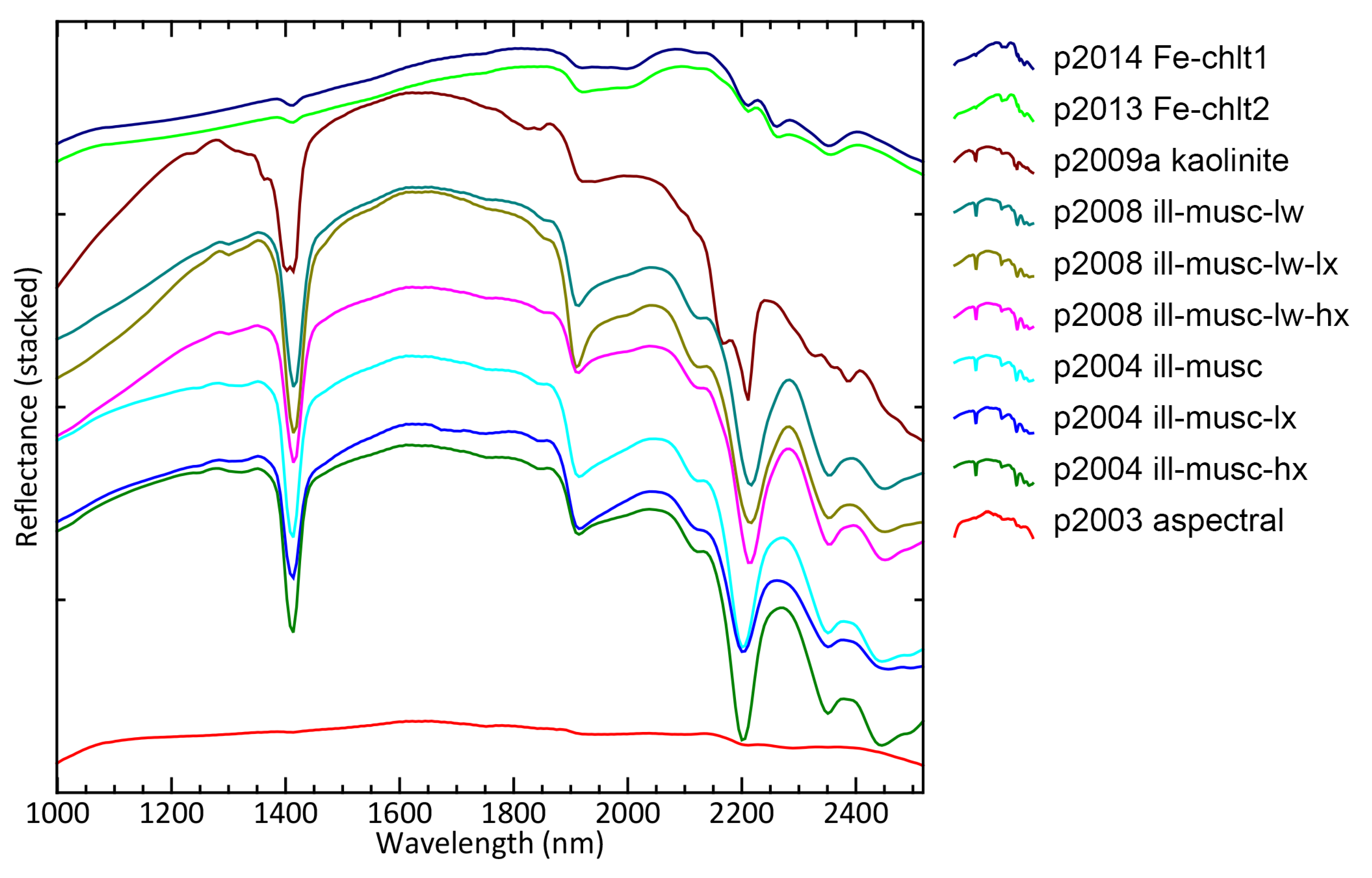
Figure 7.
Scatterplots of wavelength position versus depth of (a) deepest, (b) second deepest, and (c) third deepest absorption features between 2100-2400 nm of rock sample P2009a. Kaolinite-pixel clusters are present at ∼2209 nm in (a), ∼2166 nm in (b), and ∼2320 nm in (c).
Figure 7.
Scatterplots of wavelength position versus depth of (a) deepest, (b) second deepest, and (c) third deepest absorption features between 2100-2400 nm of rock sample P2009a. Kaolinite-pixel clusters are present at ∼2209 nm in (a), ∼2166 nm in (b), and ∼2320 nm in (c).
Chlorite-bearing rocks contain more ferrous iron, which can be seen in rock samples 9, 10 and 11 by the brownish colors (higher ferrous drop values in Figure 4d). Illite crystallinity values vary in the illite-muscovite containing rocks (Figure 5a). For instance phenocrysts in rock 2 (shown as cyan-colored clusters of pixels) have higher crystallinity values than the minerals in the matrix of the rock.
Figure 5b shows the presence of the second feature of kaolinite at 2170 nm by a change of color from blue (illite) to light blue and green (kaolinite). Kaolinite occurrences in rock 7 are shown in green.
The Shannon entropy images in Figure 5c show rock textures that results from variations in spectral mineralogy in the hyperspectral images. For example, the black clusters of pixels in rocks 2, 3 and 4 represent white mica altered phenocrysts with high crystallinity values. These white micas produce lower Shannon entropy values than the minerals in the rock matrix surrounding these phenocrysts. These differences are visible in the images in Figure 5c and they enhance the microstructure of the rock.
The results of the exploratory analysis were used to create the improved classification scheme for the rock samples and to develop the processing chain to create the mineral maps described in Section 3.2.
3.2. Mineral Maps
The mineral maps in Figure 5d resulted from the application of the processing chain, which classified wavelength images and summary products using the decision tree (Figure 2) in step 5 of the interpretation strategy. The resulting mineral maps show the distribution of illite-muscovite minerals of different composition and crystallinity, kaolinite, and chlorite minerals. These maps also show microstructural features that result from the variation in mineralogy. The spectra of rock 1 predominantly contain shallow absorption features. The pixels in the aspectral class have absorption features between 2100 and 2400 nm shallower than 0.05 reflectance (Figure 6, p2003 aspectral). The spectra with deeper features indicate white micas (yellow colors) and minerals with features between 2340 and 2400 nm (green), which are not diagnostic, but could include chalcedony. Sedimentary structures are shown by the alternation of yellow, black and green layers. Rocks 2-5 contain predominantly Al-rich white micas with wavelength positions between 2200 and 2205 nm and of varying illite-muscovite crystallinity (low crystallinity values in grey, intermediate values in yellow and high values in cyan; see Figure 6 for representative mean spectra of rock 2). The variation in crystallinity values shows the presence of xenocrysts (grey pixels in rock 2) and phenocrysts (cyan pixels in rock 2 and 3, yellow pixels in rock 4). Rocks 6-8 contain predominantly Al-poor white micas with wavelength positions between 2210 and 2215 nm and of varying illite-muscovite crystallinity (low crystallinity values in dark blue, intermediate values in orange and high values in lavender; see Figure 6 for representative mineral spectra of rock 2, 6 and 7). Rock 7 contains kaolinite in amygdales. Rocks 9-11 contain white micas and chlorites (in green, see Figure 6 for endmembers of chlorite endmembers) and their mixtures. The amygdales in rock 11 show as clusters of yellow pixels.
Visual interpretation of representative mean spectra (in Figure 6) and classification of selected reference spectra using the same decision trees in Table 4 assisted in the interpretation of the mean spectra and confirmed that the decision tree classified reference spectra in the right classes, according to the wavelength positions of absorption features and crystallinity values.
Table 4.
Classification of reference spectra from the USGS spectral library version 7 [31] using (Tab. Table 2, Figure 2). chlt=chlorite; epid=epidote; ill=illite; musc=muscovite; sw=short wavelength; lw=long wavelength; lx=low crystallinity; hx=high crystallinity
| Class | Count | Reference spectrum |
|---|---|---|
| ill-musc-sw | 2 | Muscovite_GDS113_Ruby; Muscovite_GDS113a_Ruby |
| phengite | 2 | Illite_GDS4.2_Marblehead; Illite_GDS4_Marblehead |
| epid/chlt | 5 | Chlorite_HS179.1B; Chlorite_HS179.2B; Chlorite_HS179.3B; Chlorite_HS179.4B; Chlorite_HS179.6 |
| ill-musc-hx | 3 | Muscovite_HS146.1B; Muscovite_HS146.3B; Muscovite_HS146.4B |
| ill-musc-lx | 2 | Illite_IMt-1.a; Illite_IMt-1.b_lt2um |
| ill-musc-lw-hx | 2 | Muscovite_GDS116_Tanzania; Muscovite_GDS116a_Tanzania |
| kaolinite | 3 | Kaolinite_CM9; Kaolinite_KGa-1_(wxl); Kaolinite_KGa-2_(pxl) |
4. Discussion
4.1. Strengths
The interpretation strategy presented here has the following strengths: i) The focus on the wavelength positions of absorption features, which are physical mineral properties rather than statistical measures, ii) the possibility to evaluate of spatial patterns in the different wavelength maps and summary products, iii) its versatility, iv) the possibility to the built-in expert knowledge, and v) the option to automate processing and classification steps.
Focus on wavelength positions of absorption features. The wavelength positions of absorption features in the SWIR are directly related to the energy level of atomic and molecular bonds in the crystal lattices and therefore physics based [32]. This makes them less susceptible to changing measurement conditions and matrix effects in rocks (caused by other minerals and their geological structures); they can be considered as robust indicators for the presence of minerals that contain these bonds. In addition, minor changes in bond strength caused by the substitution of Al by Fe and Mg in octahedral sites in white micas manifest as small nanometer-scale changes in absorption wavelengths of the ∼2200 nm feature [33]. These minor wavelength shifts are readily observable in wavelength images.
Evaluation of spatial patterns in wavelength maps and summary products. The possibility to evaluate spatial patterns in wavelength images and summary products (for example in Figure 3- Figure 5), allows for a direct analysis of the relationships between spectral features and geological textures and micro structures. Wavelength images (and some of the summary products) represent physical mineral properties and therefore show the distribution of physical mineral parameters, which is not the case in rule images created by measuring statistical similarity between reference and pixel spectra. Furthermore, wavelength images help to identify image noise because of typical spatial patterns created by noise, including incoherent shapes and/or striping.
Versatility. The strategy is versatile because it allows for the modification of the wavelength ranges of wavelength maps, their stretching intervals, the type of summary products to enhance specific mineralogical variation, as well as the addition of newly-developed decision trees or modification of existing trees. Processing chains can readily be adapted to create mineral maps that are specific for certain mineral assemblages and geological settings.
Incorporation of expert knowledge. The use of expert knowledge reduces uncertainty in the in the analysis and interpretation of hyperspectral images. Expert knowledge was incorporated in several steps of the interpretation strategy. The creation of wavelength images and maps, summary products and decision trees for the exploratory analysis in step 1, the exploratory analysis and interpretation of maps and spectra in step 2, the comparison with reference spectra and other mineral analyses in step 3, and the development of the improved classification scheme and decision tree to create mineral maps in step 4, all require expert knowledge about mineral reflectance spectra and hyperspectral image processing and classification, as well as geological image interpretation. However, once the processing chain for the creation of mineral maps is developed, the processing can be performed by non-expert geologists and the mineral maps can be readily understood.
Automation of processing and classification steps. All processing and classification steps in the interpretation strategy were created using HypPy software command line statements. This made it possible to automate all the steps in which images, maps and spectra were created and processed. Only the steps that required analysis and interpretation by a human operator can not be automated. Once the processing chain for the classification of the rock samples was created (in step 4 in Figure 1), the execution of the procedure is automated and applied to all hyperspectral images. The automation has the advantage that results are reproducible, the image processing and classification process become time-efficient, and the risk of human-induced errors is reduced.
4.2. Weaknesses
Weaknesses of the interpretation strategy may lie in i) the requirement for expert knowledge to develop the various classification procedures, and ii) the focus on deepest features that cause bias toward spectrally dominant minerals.
Requirement for expert knowledge to develop processing chain. Spectral geological expert-knowledge is required for the interpretation of hyperspectral image maps and spectra and for the development of a processing chain to create the mineral maps. This could be seen as a weakness because it requires investment in understanding mineral spectroscopy and the analysis and interpretation of hyperspectral images.
Bias toward dominant spectral minerals. The focus on deepest absorption features may result in bias toward the identification of minerals that produce deep absorption features and dominate the spectral mineralogy. It is important that the interpreter of the various classifications is aware of this potential bias so that the interpretation strategy is adapted to include the detection of minerals with shallow absorption features as well. One example of such strategies is the adjustment of the depth stretch of absorption features in the process of calculating wavelength maps so that shallow features are also visible. Another example is the use of multiple absorption features (including the shallower features of less dominant minerals) within specific wavelength ranges.
4.3. Application
We demonstrated the interpretation strategy on laboratory-acquired SWIR hyperspectral images of hydrothermally altered volcanic rock samples at high spatial and spectral resolution between 1000 and 2500 nm. The rock samples were coherent and intact, therefore, the spatial patterns in the distribution of spectral minerals could be evaluated and allowed the identification of sedimentary and volcanic micro structures including the presence of phenocrysts, xenocrysts and amygdales [cf., [34]. The strategy can also be applied to hyperspectral images of rock samples that are fragmented, such as rock chips resulting from drilling [35]. Focus is then less on the analysis of spatial patterns in the imagery and more on the classification of the minerals in the rock fragments.
The study has shown that the classification procedures used in the interpretation can be applied automatically to multiple images from rocks acquired from the same type of geological setting with similar mineralogical compositions using the same processing chain. Therefore, the method is suitable for an automated classification of large sets of hyperspectral imagery. The analysis and interpretation can be applied over large depth intervals with exactly the same classification procedure and with reproducible results. Care should be taken when working in different geological settings with other mineralogical assemblages. The classification procedures may have to be adjusted by comparison with complementary mineralogical analysis to include the changed mineralogical characteristics in that setting. This may result in the use of wavelength maps over different wavelength ranges, other summary products and decision trees and a modified processing chain.
The interpretation strategy was developed for academic geological research, as is shown in the study presented here, but may also be suitable where mineralogical information is required for informed decision making, for example in mineral exploration [e.g., [36] and the exploration for hydrocarbons and geothermal energy [35].
The interpretation strategy has not been tested on hyperspectral images covering other wavelength ranges (e.g., visible, near and long-wavelength infrared), on multi-spectral images and on airborne and spaceborne hyperspectral images at lower spatial resolution. Investigating the suitability of the strategy on those data sets are topics for future research.
5. Conclusions
The novel interpretation strategy presented here involves the application of a series of processing, analysis and classification steps for the extraction of geological and mineralogical information from hyperspectral images of rocks and the creation of mineral maps. The strategy is different from other commonly applied strategies since it uses physics-based criteria instead of statistical measures to create mineral maps. We demonstrated how exploratory analysis of processed hyperspectral images and comparison with complementary mineral and chemical analyses allowed the creation of a processing chain to create mineral maps from hyperspectral images of a suite of hydrothermally altered rock samples. We conclude that the interpretation strategy provides an effective means to embed expert knowledge in the interpretation of hyperspectral images of rocks and into a processing chain to create reproducible mineral maps without relying on statistical matching criteria.
Author Contributions
Conceptualization, Frank van Ruitenbeek; Formal analysis, Frank van Ruitenbeek; Funding acquisition, Frank van Ruitenbeek and Kim Hein; Investigation, Frank van Ruitenbeek and Kim Hein; Methodology, Frank van Ruitenbeek, Wim Bakker and Christoph Hecker; Resources, Kim Hein and Wijnand van Eijndthoven; Software, Wim Bakker, Harald van der Werff and Wijnand van Eijndthoven; Writing – original draft, Frank van Ruitenbeek; Writing – review & editing, Wim Bakker, Harald van der Werff, Christoph Hecker and Kim Hein.
Funding
Field data collection was financially supported by the Foundation Stichting Dr. Schürmannfonds, Grant no. 2002/22. Deep Atlas provided financial support for the implementation of the workflow methodology in HypPy.
Data Availability Statement
The hyperspectral images used in this study are available at: https://doi.org/10.17026/PT/FKIQDB.
Acknowledgments
The authors would like to acknowledge Deep Atlas B.V. for supporting the automation process of image processing steps in the workflow, Camilla Marcatelli for her assistance with the hyperspectral image acquisition, and the MSc students who used parts of the workflow in the analysis of lab-acquired hyperspectral images in their research.
Conflicts of Interest
The authors declare no conflicts of interest.
Appendix A. HypPy Command Line Syntax of Processing Steps
Preprocessing
- 1.
-
Conversion of uncalibrated radiance to reflectance image ($FILE-IN = manifest.xml file):> darkwhiteref.py -f -m $FILE-IN -o $FILE-OUT px
- 2.
-
Spatial-spectral filtering (mean7 = mean filtering by 2 spectral and 5 spatial neighbours):> median.py -f -i $FILE-IN -o $FILE-OUT -m mean7
- 3.
-
Spectral math expression to create an optional mask file for dark background pixels (expression "S1.mean()>0.05" = mean pixel-spectrum is larger than 0.05; required for wavelength mapping command):> specmath.py -o $FILE-OUT -t int16 -e "S1.mean()>0.05" $FILE-IN
Wavelength mapping
- 4.
-
Creation of wavelength image (-w 2100 -W 2400 = wavelength range from 2100 to 2400; -m div = continuum removal by division; -n 3 = calculation of 3 deepest features):> minwavelength2.py -f -i $FILE-IN -o $FILE-OUT –mask $MASKFILE -w 2100 -W 2400 -m div -n 3
- 5.
-
Creating a png image file of color composite of 1st, 2nd and 2rd deepest features in wavelength image (-R 0 -G 2 -B 4 = band numbers for the red, green and blue channels; -m SD = 2 standard deviations stretch mode):> tokml.py -i $FILE-IN -o $FILE-OUT -R 0 -G 2 -B 4 -m SD
- 6.
-
Creation of wavelength map from wavelength image (-w 2100 -W 2400 = wavelength stretch range from 2100 to 2400; -d 0 -D 0 = standard depth stretch; -l = saves legend as .png):> wavemap.py -f -i $FILE-IN -o $FILE-OUT -w 2100 -W 2400 -d 0 -D 0 -l
Summary product calculation
- 7.
-
Calculation of the summary products fedrop and illkaol (-u nan = input wavelength in nanometer; -l = creation of logfile):> otherindices.py -f -i $FILE-IN -o $FILE-OUT -u nan -l
- 8.
-
Band math formula to calculate illx from wavelength images 2100-2400nm and 1850-2100nm (Expression: `i1[1] / i2[1]’= ratio of band 1 in image 1 (wavelength image 2100-2400nm, $FILE-IN1) over band 1 in image 2 (wavelength image 1850-2100nm, $FILE-IN2)):> bandmath.py -o $FILE-OUT -e `i1[1] / i2[1]’ $FILE-IN1 $FILE-IN2
- 9.
-
Spectral math expression to calculate albedo image, i.e., the mean spectrum of each pixel (`S1.mean()’= expression to calculate mean of spectrum):> specmath.py -o $FILE-OUT -e `S1.mean()’$FILE-IN
- 10.
-
Band math formula to calculate illx from band ratio (expression: `i1(2178)/i1(2189)’= ratio of bands 2187 over 2189 nm):> bandmath.py -o $FILE-OUT -e `i1(2178)/i1(2189)’ $FILE-IN
- 11.
-
Spectral math expression to calculate Shannon entropy (expression: `(1-S1).entropy2()’= calculation of Shannon entropy):> specmath.py -o $FILE-OUT -e `(1-S1).entropy2()’ $FILE-IN
Decision tree classification
- 12.
-
Classification using decision tree ($DT) of bands 0 (b2), 1 (b3) and 2 (b7) of wavelength image ($FILE-IN):> decisiontree.py -t $DT -o $FILE-OUT -b2 $FILE-IN 0 -b3 $FILE-IN 1 -b7 $FILE-IN 2
- 13.
-
Creation of legend of classified file ($FILE-IN):> makelegend.py -i $FILE-IN
- 14.
-
Calculation of mean spectra of all classes in class file ($CLASS-IN) from reflectance image ($FILE-IN) (-o $PLOT-OUT = plot of mean spectra; -l $SPECLIB = folder with ASCII mean spectra; -r $CLASSREPORT = report of class percentages in image):> classstats.py -i $FILE-IN -c $CLASS-IN -o $PLOT-OUT -l $SPECLIB -r $CLASSREPORT
Appendix B. Wavelength Maps
Figure A1.
Wavelength maps of the hyperspectral images of the eleven rock samples: (a) wavelength map between 1300-1600 nm, (b) wavelength map between 1850-2100 nm. Rock samples: 1=P2003, 2=P2004, 3=P2005, 4=P2006, 5=P2007, 6=P2008, 7=P2009a, 8=P2010, 9=P2012, 10=P2013 and 11=P2014. See Table 3 for descriptions of the rock samples. Width of the images is 1.1 cm.
Appendix C. Decision trees
Figure A2.
Decision tree for the classification of wavelength images between 2100 and 2400 nm. The design of the tree based on expert knowledge on the wavelength position and depth of absorption features of minerals in reflectance spectra between 2100-2400 nm. Input bands are the depth of deepest absorption features between 2100 and 2400 nm (b3) and wavelength position of deepest (b2) and second deepest (b7) features. The application of this tree involves: 1) Selection of pixels with a minimum feature depth of 0.05 reflectance (pixels with shallower depth are named "aspectral"), 2) Slicing of the wavelength of deepest absorption features at 2160, 2180, 2200, 2210, 2220, 2240, 2260, 2300, 2320, 2340 and 2360 nm, 3) Subdivision of the classes with deepest absorption features i) between 2160-2180 nm by thresholding of the second deepest absorption features between 2200-2220 nm, and between 2300-2320 nm to identify alunite and/or dickite (alu_dick) and pyrophyllite (pyrophyll) respectively, ii) between 2200-2210 nm by thresholding between 2160-2180 nm to identify kaolinite (kaol), iii) between 2200-2200 nm by thresholding between 2340-2400 nm to separate illite-muscovite (musc_ill) from other minerals, iv) between 2240-2300 nm by thresholding between 2340-2400 nm to separate Fe-chlorites (Fe_chlt) from other minerals, v) between 2300-2320 nm by thresholding between 2100-2160 nm to identify carbonate minerals (dolom) between 2240-2260 nm to identify Mg-chlorite (Mg-chlt) and between 2340-2400 nm to identify amphibole and/or talc (amp-talc), vi) between 2320-2340 nm by thresholding between 2240-2260 nm to separate epidote and/or chlorite (epid_chlt) and between 2260-2300 nm to identify serpentine (serp), vii) between 2340-2360 nm by thresholding between 2220-2240 nm to separate prehnite. The resulting classes are named after a mineral when the classification scheme is specific to that mineral (e.g., class "pryrophyll" refers to pyrophyllite), else they are named "other" together with an index number (e.g., "other-1"). alu=alunite, dick=dickite, pyrophyll=pyrophyllie, kaol=kaolinite, musc=muscovite, chlt=chlorite, amp=amphybole, dolom=dolomite, epid=epidote, serp=serpentine.
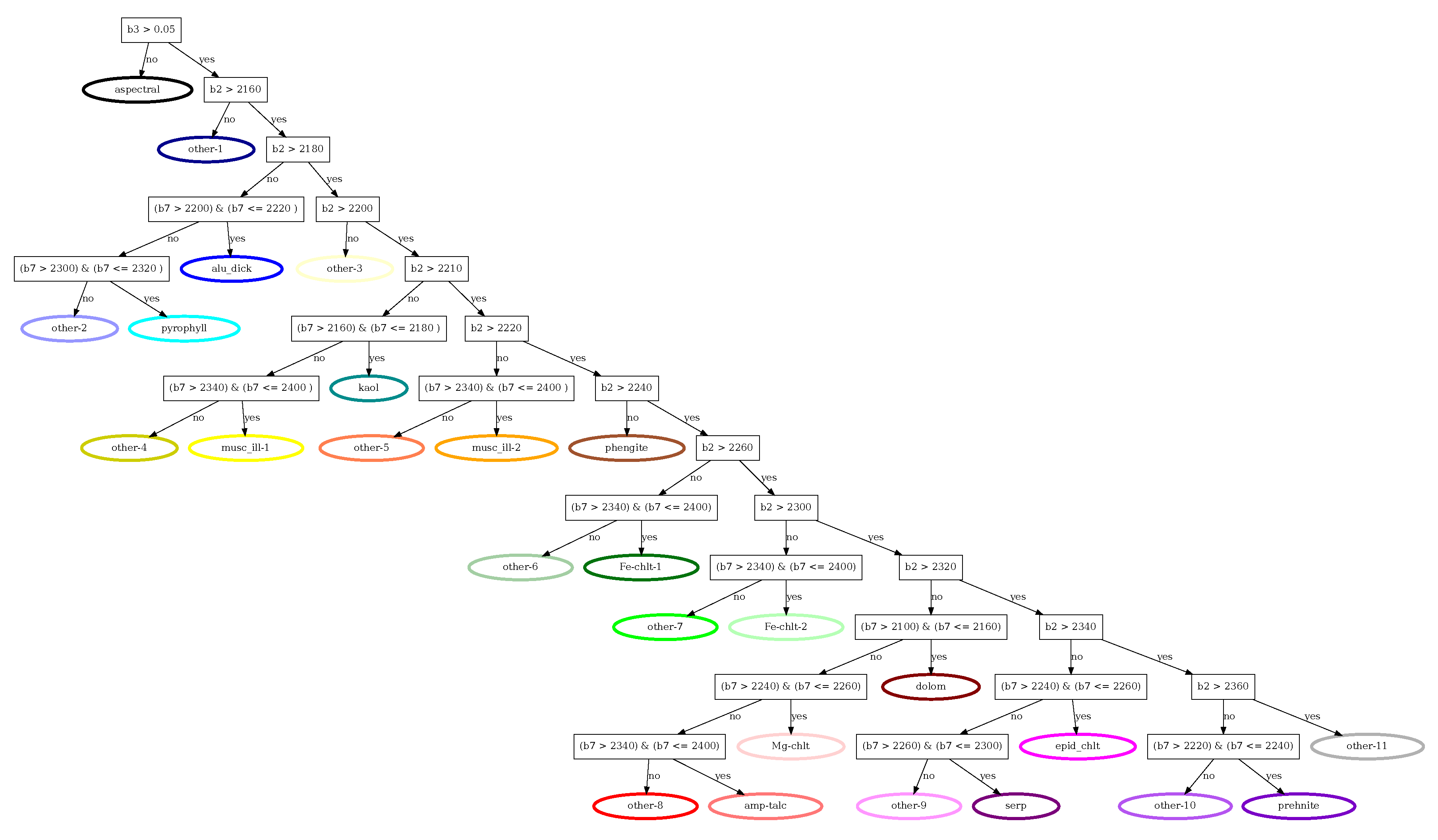
Figure A3.
Decision tree for the classification of albedo images. Input band is the albedo image (b1). The application of this tree involves the slicing of the albedo values at 0.25, 0.38 and 0.5 into different brightness classes. The thresholds are based on experience with brightness levels of similar types of rock in hyperspectral images. med=medium.
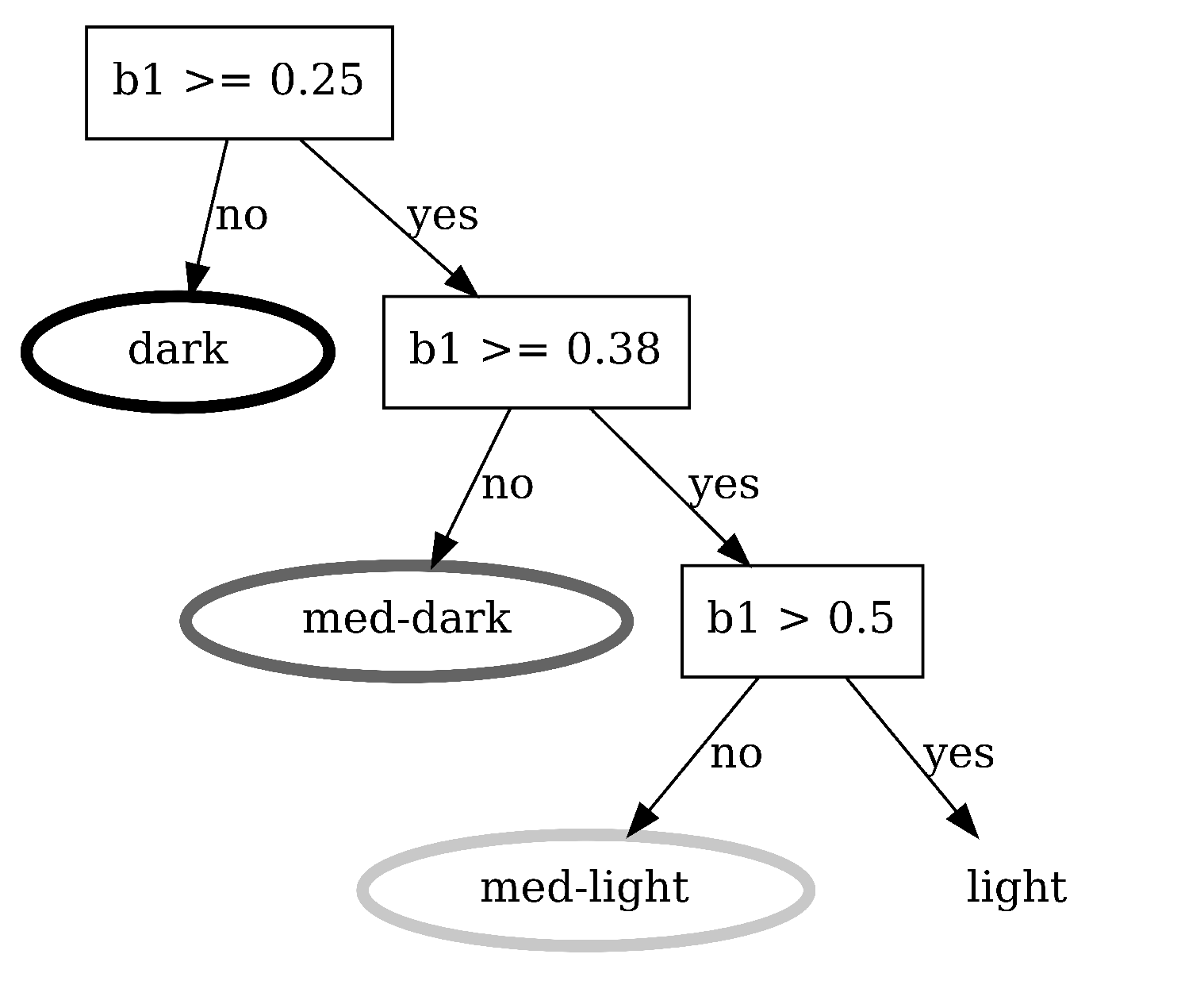
Figure A4.
Decision tree for the classification of fe-drop images. Input bands are the fedrop image (b1) and the depth (b3) and wavelength position (b2) of deepest features in the wavelength image between 2100 and 2400 nm. The application of this tree involves 1) Selection of pixels with a minimum feature depth of 0.05 reflectance (pixels with shallower depth are named "aspectral"), 2) Thresholding of wavelengths of deepest absorption features between 2100-2400 nm, and 3) Slicing of the fedrop values at 1.1, 1.2, 1.3, 1.4, and 1.5. The fedrop thresholds are based on experience with fedrop values in hyperspectral images of similar types of rock. med=medium.
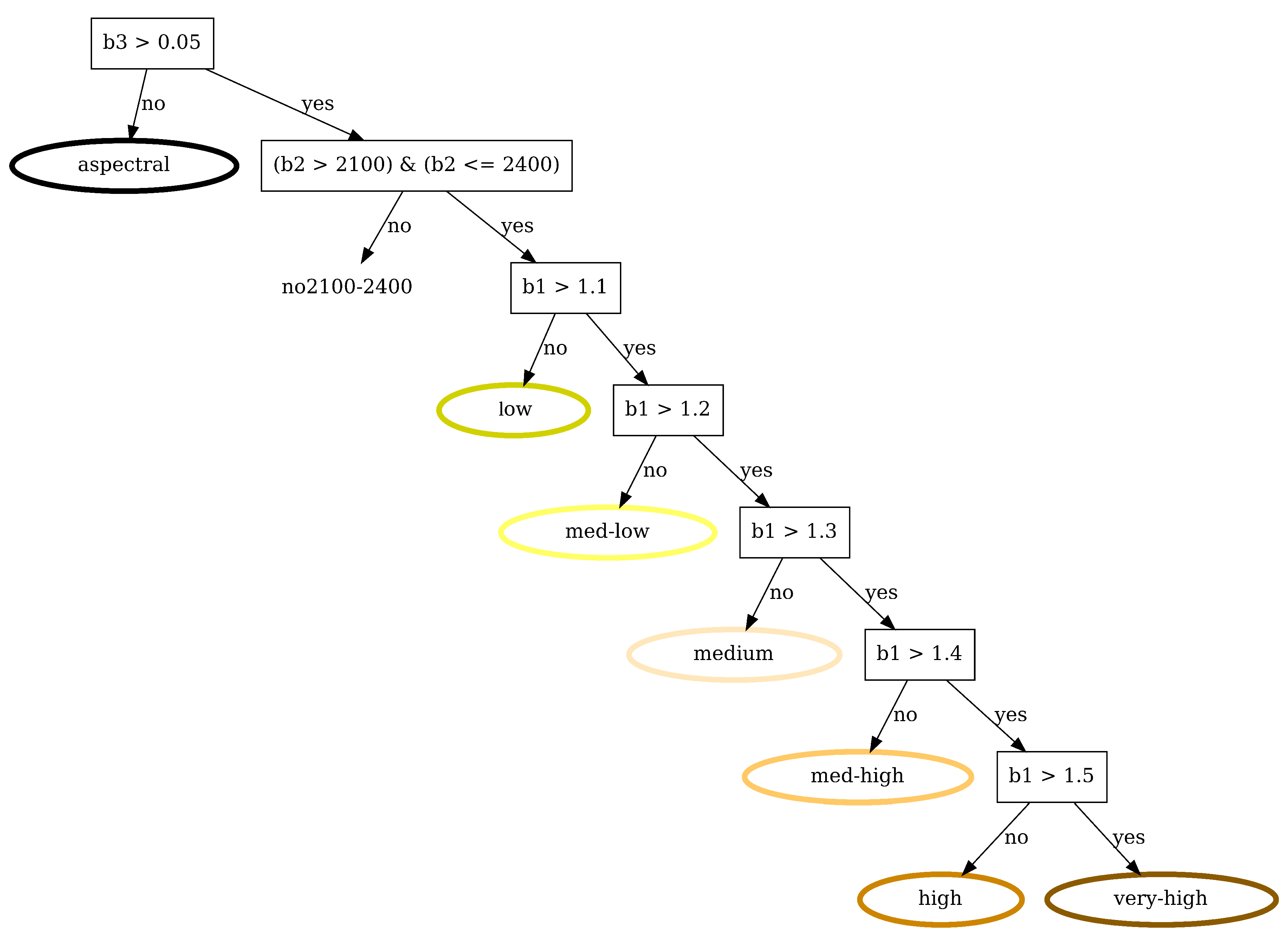
Figure A5.
Decision tree for the classification of illx images. Input bands are the illx image (b1) and the depth (b3) and wavelength position (b2) of deepest features in the wavelength image between 2100 and 2400 nm. The application of this tree involves 1) Selection of pixels with a minimum feature depth of 0.05 reflectance (pixels with shallower depth are named "aspectral"), 2) Thresholding of wavelengths of deepest absorption features between 2185-2225 nm to select only minerals with deepest Al-OH features in this range, and 3) Slicing of the illite crystallinity values at 0.25, 0.33, 0.5, 1, 2, 3, 4. The illite crystallinity thresholds are based on experience with crystallinity values in hyperspectral images of similar types of rock. Classes with similar mineral names are followed by a number. smect=smectite, ill=illite, hx=high crystallinity, musc=muscovite.
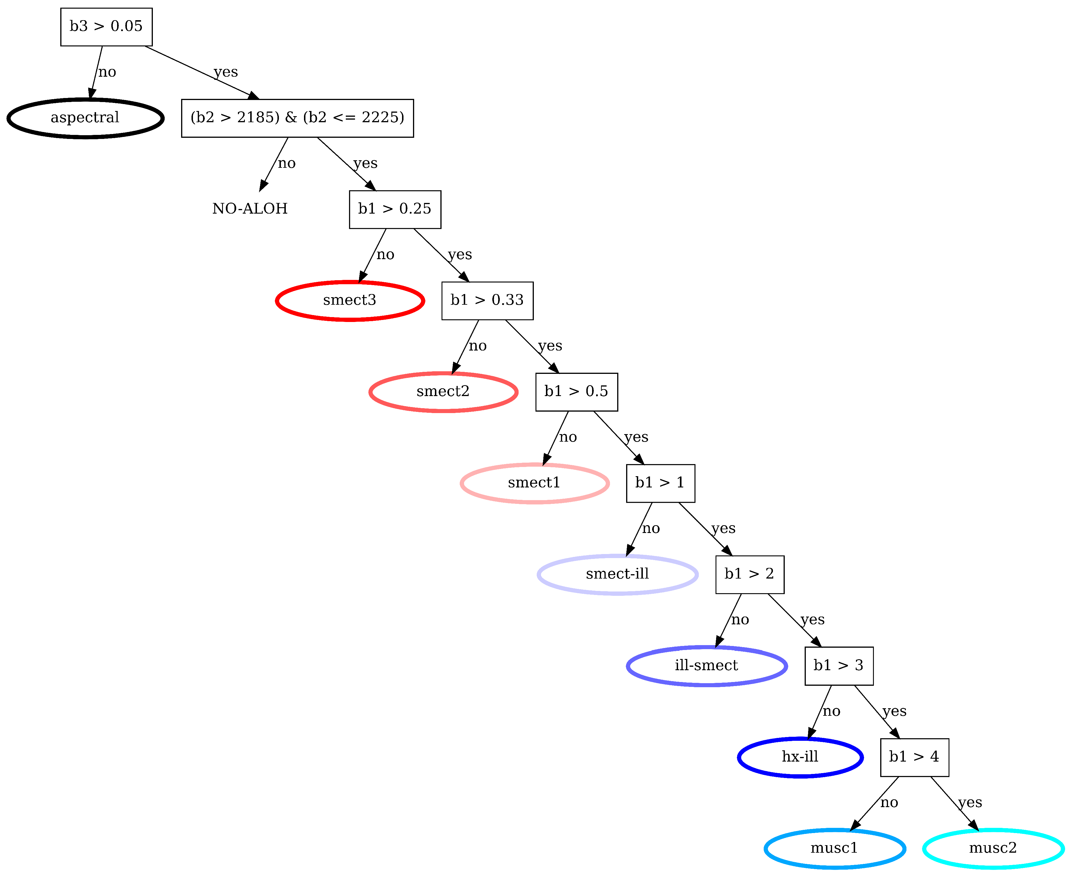
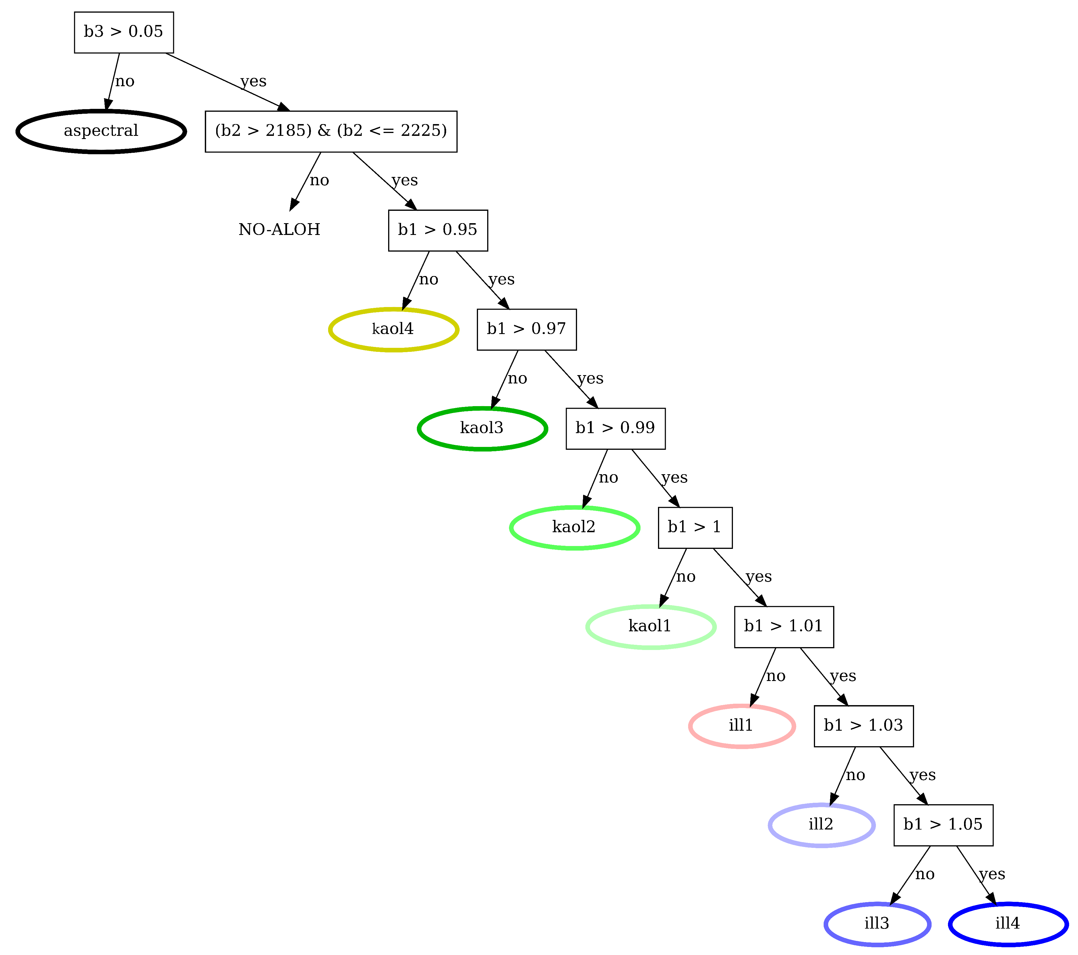
Figure A6.
Decision tree for the classification of illkaol images. Input bands are the illkaol image (b1) and the depth (b3) and wavelength position (b2) of deepest features in the wavelength image between 2100 and 2400 nm. The application of this tree involves 1) Selection of pixels with a minimum feature depth of 0.05 reflectance (pixels with shallower depth are named "aspectral"), 2) Thresholding of wavelengths of deepest absorption features between 2185-2225 nm to select only minerals with deepest Al-OH features in this range, and 3) Slicing of the illite_kaolinite values at 0.95, 0.97, 0.99, 1, 1.01, 1.03, and 1.05. The illite_kaolinite thresholds are based on the analysis of reflectance spectra of illite and kaolinite mixtures. Classes with similar mineral names are followed by a number. kaol=kaolinite, ill=illite.
References
- Acosta, I.C.C.; Khodadadzadeh, M.; Tolosana-Delgado, R.; Gloaguen, R. Drill-core hyperspectral and geochemical data integration in a superpixel-based machine learning framework. IEEE Journal of Selected Topics in Applied Earth Observations and Remote Sensing 2020, 13, 4214–4228. [Google Scholar] [CrossRef]
- Baissa, R.; Labbassi, K.; Launeau, P.; Gaudin, A.; Ouajhain, B. Using HySpex SWIR-320m hyperspectral data for the identification and mapping of minerals in hand specimens of carbonate rocks from the Ankloute Formation (Agadir Basin, Western Morocco). Journal of African Earth Sciences 2011, 61, 1–9. [Google Scholar] [CrossRef]
- Dalm, M.; Buxton, M.; Van Ruitenbeek, F. Discriminating ore and waste in a porphyry copper deposit using short-wavelength infrared (SWIR) hyperspectral imagery. Minerals engineering 2017, 105, 10–18. [Google Scholar] [CrossRef]
- Kruse, F. Identification and mapping of minerals in drill core using hyperspectral image analysis of infrared reflectance spectra. International Journal of Remote Sensing 1996, 17, 1623–1632. [Google Scholar] [CrossRef]
- Mathieu, M.; Roy, R.; Launeau, P.; Cathelineau, M.; Quirt, D. Alteration mapping on drill cores using a HySpex SWIR-320m hyperspectral camera: Application to the exploration of an unconformity-related uranium deposit (Saskatchewan, Canada). Journal of Geochemical Exploration 2017, 172, 71–88. [Google Scholar] [CrossRef]
- Turner, D.; Groat, L.A.; Rivard, B.; Belley, P.M. Reflectance spectroscopy and hyperspectral imaging of sapphire-bearing marble from the beluga occurrence, Baffin Island, Nunavut. The Canadian Mineralogist 2017, 55, 787–797. [Google Scholar] [CrossRef]
- Van der Meer, F.D.; Van der Werff, H.M.; Van Ruitenbeek, F.J.; Hecker, C.A.; Bakker, W.H.; Noomen, M.F.; Van Der Meijde, M.; Carranza, E.J.M.; De Smeth, J.B.; Woldai, T. Multi-and hyperspectral geologic remote sensing: A review. International Journal of Applied Earth Observation and Geoinformation 2012, 14, 112–128. [Google Scholar] [CrossRef]
- Clark, R.N. Spectroscopy of rocks and minerals, and principles of spectroscopy. In Manual of Remote sensing; Rencz, A.N., Ed.; John Wiley and Sons: New York, 1999. [Google Scholar]
- Laukamp, C.; Rodger, A.; LeGras, M.; Lampinen, H.; Lau, I.C.; Pejcic, B.; Stromberg, J.; Francis, N.; Ramanaidou, E. Mineral physicochemistry underlying feature-based extraction of mineral abundance and composition from shortwave, mid and thermal infrared reflectance spectra. Minerals 2021, 11, 347. [Google Scholar] [CrossRef]
- Asadzadeh, S.; de Souza Filho, C.R. A review on spectral processing methods for geological remote sensing. International Journal of Applied Earth Observation and Geoinformation 2016, 47, 69–90. [Google Scholar] [CrossRef]
- Kurz, T.H.; Buckley, S.J.; Howell, J.A. Close-range hyperspectral imaging for geological field studies: Workflow and methods. International Journal of Remote Sensing 2013, 34, 1798–1822. [Google Scholar] [CrossRef]
- Rodger, A.; Fabris, A.; Laukamp, C. Feature extraction and clustering of hyperspectral drill core measurements to assess potential lithological and alteration boundaries. Minerals 2021, 11, 136. [Google Scholar] [CrossRef]
- Wolfe, J.; Black, S. Hyperspectral analytics in ENVI. Available at: https://www.spectroexpo.com/wp-content/uploads/2021/03/Hyperspectral_Whitepaper.pdf; accessed 2-April-2025, 2018.
- Kleynhans, T.; Messinger, D.W.; Delaney, J.K. Towards automatic classification of diffuse reflectance image cubes from paintings collected with hyperspectral cameras. Microchemical Journal 2020, 157, 104934. [Google Scholar] [CrossRef]
- Kruse, F.; Letkoff, A.; Boardmann, J.; Heidebrecht, K.; Shapiro, A.; Barloon, P.; Goetz, A. The spectral image processing system (SIPS) – interactive visualization and analysis of imaging spectrometer data. Remote Sensing of Environment 1993, 44, 145–163. [Google Scholar] [CrossRef]
- Boardman, J.W.; Kruse, F.A. Analysis of imaging spectrometer data using n-dimensional geometry and a mixture-tuned matched filtering approach. IEEE Transactions on Geoscience and Remote Sensing 2011, 49, 4138–4152. [Google Scholar] [CrossRef]
- Bioucas-Dias, J.M.; Plaza, A.; Dobigeon, N.; Parente, M.; Du, Q.; Gader, P.; Chanussot, J. Hyperspectral unmixing overview: Geometrical, statistical, and sparse regression-based approaches. IEEE journal of selected topics in applied earth observations and remote sensing 2012, 5, 354–379. [Google Scholar] [CrossRef]
- Paoletti, M.; Haut, J.; Plaza, J.; Plaza, A. Deep learning classifiers for hyperspectral imaging: A review. ISPRS Journal of Photogrammetry and Remote Sensing 2019, 158, 279–317. [Google Scholar] [CrossRef]
- Hecker, C.; Van der Meijde, M.; Van Der Werff, H.; Van Der Meer, F.D. Assessing the influence of reference spectra on synthetic SAM classification results. IEEE Transactions on Geoscience and Remote Sensing 2008, 46, 4162–4172. [Google Scholar] [CrossRef]
- Bakker, W.; van Ruitenbeek, F.; van der Werff, H.; Hecker, C.; Dijkstra, A.; van der Meer, F. Hyperspectral Python – HypPy. Algorithms 2024, 17, 337. [Google Scholar] [CrossRef]
- Van Ruitenbeek, F. High-resolution, laboratory acquired hyperspectral images of rock samples from the footwall of the Kangaroo Caves Cu-Zn deposit, Pilbara, Western Australia. 2004. [CrossRef]
- Hecker, C.; van Ruitenbeek, F.J.; van der Werff, H.M.; Bakker, W.H.; Hewson, R.D.; van der Meer, F.D. Spectral absorption feature analysis for finding ore: A tutorial on using the method in geological remote sensing. IEEE Geoscience and Remote Sensing Magazine 2019, 7, 51–71. [Google Scholar] [CrossRef]
- Van Ruitenbeek, F.J.; Bakker, W.H.; van der Werff, H.M.; Zegers, T.E.; Oosthoek, J.H.; Omer, Z.A.; Marsh, S.H.; van der Meer, F.D. Mapping the wavelength position of deepest absorption features to explore mineral diversity in hyperspectral images. Planetary and Space Science 2014, 101, 108–117. [Google Scholar] [CrossRef]
- Viviano, C.; Seelos, F.; Murchie, S.; Kahn, E.; Seelos, K.; Taylor, H.; Taylor, K.; Ehlmann, B.; Wiseman, S.; Mustard, J.; et al. Revised CRISM spectral parameters and summary products based on the currently detected mineral diversity on Mars. Journal of Geophysical Research: Planets 2014, 119, 1403–1431. [Google Scholar] [CrossRef]
- Pontual, S.; Merry, N.; Gamson, P. GMEX, Practical applications handbook; AusSpec International Pty. Ltd., 1997.
- Dalm, M.; Buxton, M.W.; van Ruitenbeek, F.J.; Voncken, J.H. Application of near-infrared spectroscopy to sensor based sorting of a porphyry copper ore. Minerals Engineering 2014, 58, 7–16. [Google Scholar] [CrossRef]
- Van Ruitenbeek, F.; Goseling, J.; Bakker, W.H.; Hein, K.A. Shannon entropy as an indicator for sorting processes in hydrothermal systems. Entropy 2020, 22, 656. [Google Scholar] [CrossRef] [PubMed]
- Safavian, S.R.; Landgrebe, D. A survey of decision tree classifier methodology. IEEE Transactions on Systems, Man, and Cybernetics 1991, 21, 660–674. [Google Scholar] [CrossRef]
- Van Ruitenbeek, F.; van der Werff, H.; Hein, K.; van der Meer, F. Detection of pre-defined boundaries between hydrothermal alteration zones using rotation-variant template matching. Computers & Geosciences 2008, 34, 1815–1826. [Google Scholar] [CrossRef]
- Van Hinsberg, C. An integrated study of hydrothermal white mica in the footwall of the Kangaroo Caves VMS deposit, Western Australia 2010. Master’s thesis, Available at https://studenttheses.uu.nl/bitstream/handle/20.500.12932/5473/Thesis.pdf?sequence=1; accessed 2-April-2025.
- Kokaly, R.; Clark, R.; Swayze, G.; Livo, K.; Hoefen, T.; Pearson, N.; Wise, R.; Benzel, W.; Lowers, H.; Driscoll, R.; et al. USGS spectral library version 7 data: US Geological Survey data release. United States Geological Survey (USGS): Reston, VA, USA 2017, 61. [Google Scholar] [CrossRef]
- Hunt, G.R. Spectral signatures of particulate minerals in the visible and near infrared. Geophysics 1977, 42, 501–513. [Google Scholar] [CrossRef]
- Duke, E. Near infrared spectra of muscovite, Tschermak substitution, and metamorphic reaction progress: Implications for remote sensing. Geology 1994, 22, 621–624. [Google Scholar] [CrossRef]
- Van Ruitenbeek, F.; van der Werff, H.; Bakker, W.; van der Meer, F.; Hein, K. Measuring rock microstructure in hyperspectral mineral maps. Remote Sensing of Environment 2019, 220, 94–109. [Google Scholar] [CrossRef]
- Savitri, K.; Hecker, C.; van Ruitenbeek, F.; Sihotang, M. A decision-tree classifier for infrared imaging spectroscopy with geothermal expert knowledge in preparation.
- Martynenko, S.; Tuisku, P.; van Ruitenbeek, F.; Hein, K. High-resolution short-wave infrared hyperspectral characterization of alteration at the Sadiola Hill gold deposit, Mali, Western Africa. In Proceedings of the 15th Biennial Meeting of the Society for Geology Applied to Mineral Deposits: Life with ore deposits on Earth. University of Glasgow, 2019, p. 1325. [Available at https://ris.utwente.nl/ws/portalfiles/portal/138697676/283_SGA_Martynenko_et_al_2019_Final.pdf; accessed 2-April-2025].
| 1 | ENVI is a trademark of NV5 Geospatial Solutions, Inc. |
Figure 1.
Strategy for the interpretation of SWIR hyperspectral imagery of rock samples.
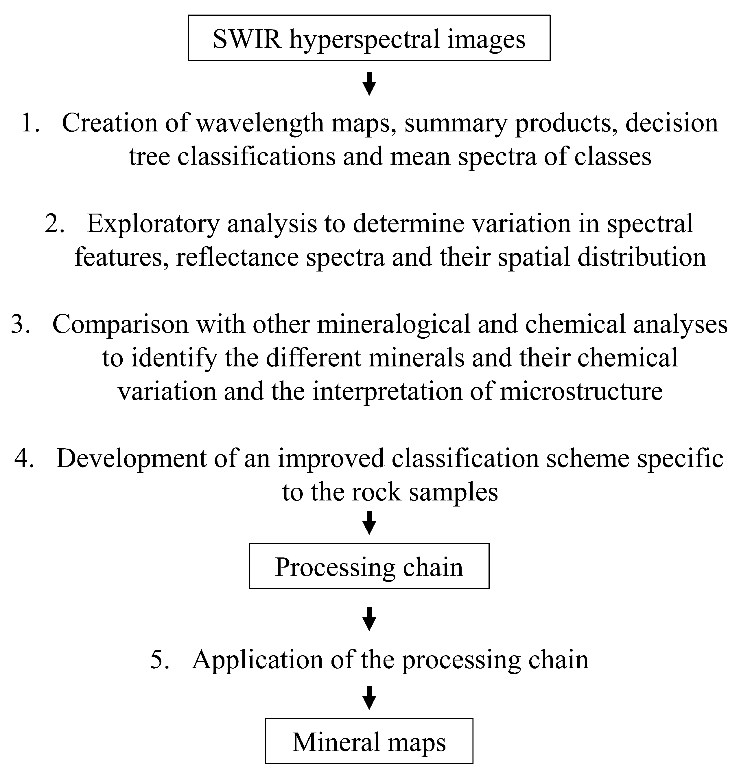
Table 1.
Description of summary products. See Appendix A for an overview of command-line syntax to create the summary products.
Table 1.
Description of summary products. See Appendix A for an overview of command-line syntax to create the summary products.
| Name | Description | Interpretation |
|---|---|---|
| Albedo | Mean reflectance value of all bands in a pixel spectrum. | Brightness. |
| Ferrous drop (fedrop) | Ratio of reflectance bands at 1600 over 1310 nm [25]. | Indication of ferrous iron in minerals, e.g. illite and carbonates. High values indicate abundant ferrous iron in the mineral. |
| Illite crystallinity (illx) | Ratio of the depths of deepest features between 2100-2400 and 1850-2100 nm, i.e., the depths of the Al-OH feature and water features of smectite-illite-muscovite minerals [25]. | Indication of the degree of ordering of the mineral (e.g., [26]); High values indicate relatively high degrees of ordering. |
| Illite-kaolinite (illkaol) | Ratio of reflectance bands at 2164 over 2180 nm. The 2164 nm band is positioned at the second deepest feature of the doublet feature of kaolinite and the 2180 nm band is position at the high between the double feature [25]. | Indication for the relative amounts of illite (high values) and kaolinite (low values). Note that the values are affected by the type of kaolinite in the rock and the center wavelengths of the bands of the hyperspectral camera used. |
| Shannon entropy | Measure from information theory: |
It measures the deviation from a flat horizontal spectrum. A flat spectrum results in highest Shannon entropy values. Spectra with few but deep features produce low values. |
Disclaimer/Publisher’s Note: The statements, opinions and data contained in all publications are solely those of the individual author(s) and contributor(s) and not of MDPI and/or the editor(s). MDPI and/or the editor(s) disclaim responsibility for any injury to people or property resulting from any ideas, methods, instructions or products referred to in the content. |
© 2025 by the authors. Licensee MDPI, Basel, Switzerland. This article is an open access article distributed under the terms and conditions of the Creative Commons Attribution (CC BY) license (http://creativecommons.org/licenses/by/4.0/).
Copyright: This open access article is published under a Creative Commons CC BY 4.0 license, which permit the free download, distribution, and reuse, provided that the author and preprint are cited in any reuse.


