Submitted:
02 May 2025
Posted:
06 May 2025
Read the latest preprint version here
Abstract
The global burden of diabetes mellitus (DM) continues to escalate, posing significant challenges to healthcare systems worldwide. This study compares machine learning (ML) and deep learning (DL) methods and their ensembles for predicting the health outcomes of diabetic patients. This work aims to find the best solutions that strike a compromise between computational economy and good prediction accuracy. The study systematically assessed a range of predictive models, including sophisticated DL techniques and conventional ML algorithms, based on computational efficiency and performance indicators. The study assessed prediction accuracy, processing speed, scalability and resource consumption, and interpretability using publicly accessible diabetes datasets. It methodically evaluates the selected models using key performance indicators (KPIs), training times, and memory usage. DT achieved the highest F1-score of 0.98, indicating excellent overall performance in balancing precision and recall. However, the RF model demonstrated higher accuracy on the hospital dataset. The results highlight how lightweight, interpretable ML models work in resource-constrained environments and for real-time health analytics. The study also compares its results with existing prediction models, confirming the benefits of selected ML approaches in enhancing diabetes-related medical outcomes. This study is substantial for practical implementation, providing a reliable and efficient framework for automated diabetes prediction to support proactive disease management techniques and tailored treatment.
Keywords:
deep learning
; diabetes mellitus
; diabetes prediction
; healthcare management outcomes
; machine learning
; performance indicators
1. Introduction
The hallmark of diabetes mellitus (DM), a chronic metabolic disease, is persistent hyperglycemia brought on by either decreased insulin action, insulin secretion, or both. Diabetes mellitus has become a pandemic in prevalence, impacting millions of people globally and dramatically raising morbidity, death, and medical costs of patients. For DM to be effectively managed, major complications like retinopathy, neuropathy, and cardiovascular diseases need to be avoided, and healthcare costs be significantly reduced. Accurate prediction and early diagnosis of diabetes and its related health outcomes are crucial [1,2]. Machine learning (ML) and deep learning (DL) techniques are now essential for delivering predictive insights, facilitating individualized patient care, and supporting clinical decision-making processes with high precision due to improvements in processing power and data availability [3,4,5]. Obesity, changes in lifestyle, and genetic susceptibility have all been implicated in the sharp rise in diabetes incidence. Diabetes can cause serious consequences, such as renal failure, neuropathy, and cardiovascular disorders if it is not treated or is not adequately controlled [6,7].
International Diabetes Foundation (IDF) has reported the rapid rise of people with diabetes aged 18 to 79 years from 4.7% to 8.5% within three decades from 1980 to 2015. The prevalence in 2019 increased to an estimated percentage of 9.3% (463 million) and is projected to rise to 10.2% (578 million) by 2030 and 10.9% (700 million) by 2045 respectively [2,8]. This indicates a serious problem for both developed and developing countries. China, India, and the United States of America are the most impacted nations, although this rise is unevenly spread, with estimates of 143% in Africa (undiagnosed cases) and 15% in Europe [8].
Early identification and precise diabetes prediction are essential for prompt management and better patient outcomes, given the disease's increasing cost on healthcare systems [9,10,11]. Wearable technology combined with powerful ML and DL algorithms has enabled real-time glucose monitoring and insulin adjustment, significantly enhancing patients' liberation and lifestyle [12]. Recent research has proven that ML and DL techniques have evolved in this area. These case studies demonstrate industry advancements while laying the groundwork for future advancements [13]. DL-based prediction models have also revealed remarkable accuracy in detecting early signs and progressions of DM-related issues, such as retinopathy, neuropathy, and nephropathy.
On the other hand, healthcare systems are designed to improve sickness detection and diagnosis while simultaneously providing patients with the essentials for optimum health [13,14]. Concerns over the quality of care offered by the healthcare system and the availability of treatment resources are common among patients [15]. Most people who would immediately benefit from better healthcare systems are those who have serious illnesses, including diabetes, hypertension, and irregular blood sugar levels [16]. A healthy society must prioritize health and healthcare. Hence, it is imperative to use state-of-the-art techniques to track the development of diabetes. Encouraging a healthy population and reducing the risk of illnesses like diabetes in future generations enables the development of novel techniques or hybrids that may be used in healthcare systems to improve the quality of life [17,18,19,20].
With their automated, data-driven insights that can improve clinical decision-making, ML and DL models have become potent medical diagnosis and prediction technologies [21,22]. While DL models like convolutional neural networks (CNNs) and recurrent neural networks (RNNs) offer sophisticated feature extraction capabilities, a variety of ML models, such as decision trees (DT), random forest (RF), logistic regression (LR), and support vector machines (SVM), have been extensively utilized for diabetes prediction. Research is ongoing to determine how well these models perform in comparison regarding accuracy, dependability, and computing economy.
This study focuses on two main research topics. The first centres around the differences in accuracy and reliability of ML and DL models in predicting diabetic patient outcomes across various healthcare settings. The second one compares ML, DL, and ensemble models regarding processing time and computational efficiency when applied to selected datasets for diabetes mellitus personalized medicine. This demonstrate the effectiveness of various ML, DL, and ensemble models in diagnosing diabetes, tracking its progression, and evaluating performance indicators by analyzing multiple datasets and comparing different predictive models.
The rest of the paper is organized into sections as follows: Section 2 presents the review of previous related literature addressing diabetes prediction, Section 3 provides an overview of the methodology, datasets used, including data preprocessing performance metrics and the models employed in this study; Section 4 presents the results of each model, highlighting their respective metrics and time efficiency; Section 5 presents a detail discussion of the results and the comparative analysis; Section 6 provides the conclusion to the study and future direction. The paper also presents a report on the datasets used.
2. Related Works
2.1. Synopsis of Diabetes Mellitus
The term "diabetes" describes a group of metabolic disorders characterized by high blood sugar levels caused by inadequate insulin synthesis, use, or both [23]. Chronic hyperglycemia is linked to long-term damage and dysfunction of organs such as the heart, blood vessels, kidneys, eyes, and nerves [23,24]. Individuals with diabetes have varying effects based on their age, income, race, and ethnicity. Environmental and genetic factors are catalysts for diabetes, resulting in insulin resistance and beta-cell death [25,26,27].
To prevent comorbidities such as cardiovascular disease, neuropathy, and retinopathy, diabetes care entails initial identification and aggressive control. Diabetes is a complicated condition with a tendency to develop silently due to lifestyle, environmental, and hereditary factors [9]. Early indicators of prediabetic diseases are often misrepresented by traditional diagnostic and treatment techniques, which can increase healthcare expenses and delayed interventions. Thus, new methods for anticipating and controlling diabetes are crucial for reducing its impact on people and enhancing positive world health outcomes [24,28]. Type 1 diabetes mellitus (T1DM), type 2 diabetes mellitus (T2DM), and gestational diabetes mellitus (GDM) are the three general forms of diabetes mellitus [29]. The hallmark of T1DM, also known as insulin-dependent diabetes, is the autoimmune destruction of the pancreatic beta-cells, which leads to insufficient insulin production. T1DM affects 5–10% of people with diabetes. Ketoacidosis, or high blood acid due to ketones, is often the initial sign of T1DM, which can develop slowly in adults or swiftly in children. It is one of the irreversible types. T1DM is becoming more common worldwide at a rate of 3% every year, affecting both sexes equally and leading to a sharp decline in life expectancy [29,30].
Non-insulin-dependent diabetes is another name for type 2 diabetes (T2DM). It is characterized by beta-cell malfunction and insulin resistance [29,30]. T2DM accounts for 90 to 95 percent of all diabetes cases. The body creates more insulin to compensate for the deficiency; nevertheless, beta-cell activity progressively decreases, leading to insulin insufficiency [31]. T2DM is associated with aging, obesity, sedentary lifestyles, high blood pressure, impaired lipid metabolism, and genetic factors. Ethnicity, which is more prevalent in some racial groups, is another aspect [31,32,33].
Pregnancy-related hyperglycemia is a common side effect of gestational diabetes mellitus (GDM) [30,34]. Despite impacting the mother and the foetus, it is frequently controllable with medicine, food, and exercise. GDM risk factors include obesity, advanced maternal age, and a history of glucose intolerance. Women with GDM have a greater lifetime risk of developing T2DM diabetes. Although there are differences in international diagnostic methods for GDM, early detection is crucial for therapy and issue prevention [35,36].
2.2. Existing Comparative Analysis of ML, DL, and Ensemble Models for DM Prediction
By extracting information from publicly available datasets and comparing various ML, DL and ensemble techniques for improved health outcomes based on accuracy, F1-score and computation time, a few researchers have made substantial contributions to the study of DM prognosis, progression, and therapy. On this wise, the scope of this study is primarily to perform a comparative analysis of several ML, DL, and ensemble models to predict the diabetic health outcomes of patients using different datasets. The comparative process would focus on the differences in accuracy, F1-score, and reliability between ML and DL models in predicting diabetic patient outcomes across various healthcare settings, as well as comparing these models and their ensembles regarding processing time and computational efficiency.
Firstly, Mahajan et al. [37] uses 16 datasets from the UCI Machine Learning Repository and Kaggle to provide a thorough comparative analysis of 15 ensemble ML approaches for illness prediction. Heart disease, liver problems, diabetes, renal disease, and skin cancer are the five main chronic illnesses that are the subject of this study. The authors evaluated the performance of various bagging, boosting, and stacking ensemble variations using various measures, including accuracy, precision, recall, F1 score, AUC, and AUPRC.
To guarantee strong model performance, datasets are subjected to thorough preparation as part of the technique, which includes data cleaning, normalization, and hyperparameter tuning. According to experimental data, stacking techniques consistently performed better than alternative ensemble approaches, especially multi-level and classical stacking. Regarding accuracy and AUC, stacking variants performed the best across all datasets with the highest frequency, whereas Logit Boost performed the worst. The results show that ensemble learning (stacking) can greatly improve prediction accuracy in illness detection by utilising the advantages of several classifiers. Researchers and practitioners may use this work's valuable insights to help choose the best ensemble methodologies for creating accurate and dependable illness prediction systems, eventually enhancing patient outcomes in healthcare settings.
To predict early-stage diabetes, Flores et al. [38] compares various ML approaches, highlighting the need for early detection for efficient disease treatment. To decrease dimensionality and eliminate less important qualities, the study initially uses a relief-based feature selection approach on a dataset of clinical and demographic characteristics gathered from diabetes patients in Bangladesh. Improving the prediction models' accuracy and efficiency requires this preprocessing step. The study looks at three main classifiers: Support Vector Machines (SVM), Random Forest (RF), and Neural Networks (NN). The models are assessed using a 10-fold cross-validation method to ensure reliable performance evaluation on unseen data. Performance indicators, including recall, specificity, accuracy, and precision were computed for every classifier. According to their results, the RF model performs better than the other models, attaining a 98.5% accuracy rate and greater precision, recall, and specificity. On the other hand, the prediction performance of NN and SVM models is slightly worse. The authors demonstrate how ensemble learning techniques, particularly RF, may manage complex feature interactions and non-linear connections in medical data. It also emphasizes how crucial thorough validation procedures and efficient feature selection are to creating trustworthy diagnostic tools. To improve early-stage diabetes prediction further, the authors suggest more study using hybrid models and larger datasets.
Using the PIMA Indian Diabetes Dataset (PIDD), Gupta et al. [39] compares the effectiveness of DL and quantum ML (QML) for diabetes prediction. The study offers two prognostic models to help doctors deal with the growing worldwide burden of diabetes. Several data preparations were performed to improve model performance, such as normalization, missing value imputation, and outlier rejection. The QML model uses a variational quantum circuit with adjustable hyperparameters, whilst the DL model is built as a multilayer perceptron with four hidden layers and optimized via root mean square propagation (RMSprop). By obtaining a precision of 0.90, accuracy of 0.95, and an F1 score of 0.93, as opposed to lower values for the QML model, the DL model surpasses the QML model, according to a thorough evaluation utilizing metrics including precision, accuracy, recall, F1 score, and diagnostic odds ratio. The results indicate that the DL approach presently provides better performance for diabetes prediction, even with the promising elements of quantum approaches.
Using the PIMA Indian Diabetes dataset, eight ML classifiers were compared for early diabetes prediction. To assess how well they predict diabetes, Aggarwal et al. [40] used Logistic Regression, Decision Tree, AdaBoost, Gradient Boosting, K-Nearest Neighbours (KNN), RF, SVM, and Naive Bayes (NB). Their study uses assessment criteria, including accuracy, confusion matrix, and F1 score, to describe the technique and performance of each classifier. Notably, the outcomes show that the NB model attains the maximum accuracy out of the methods evaluated. A thorough history of diabetes is also given in the article, along with an explanation of its many forms and related consequences and the need for early detection. To enable better clinical decision-making and patient care, the study compares these various ML techniques to determine the best effective algorithm for diabetes prediction. The results offer insightful information on medical diagnostics and ML applications in the healthcare industry.
Comparing DL and ML techniques for early-stage diabetes prediction, a benchmark UCI diabetes dataset with 16 features from 520 patients, implanting 416 training and 104 testing sets, respectively, were used by Refat et al. [41]. Performance criteria, including accuracy, recall, F1-score, ROC-AUC, and execution time were used to assess a variety of classifiers, including Extreme Gradient Boosting (XGBoost), Decision Tree (DT), RF, SVM, Multi-layer Perceptron (MLP), and Logistic Regression (LR). According to experimental data, the authors concluded that the XGBoost classifier performs better than other models, with a testing accuracy of 99.0% and training accuracy of 99.99%. The significance of preprocessing procedures and feature selection for enhancing diagnostic accuracy are emphasized in this study. Despite encouraging results, the study admits limitations because of the small dataset size and recommends that future research concentrate on obtaining larger datasets and investigating new predicting markers for improved early diabetes identification.
Swathy & Saruladha [42] delivered a thorough comparison of several categorization and prediction methods for cardiovascular diseases (CVD), one of the comorbidities of DM, using various ML and DL approaches. The authors highlight the importance of early identification to enhance clinical outcomes, acknowledging CVD as a primary cause of death. The study divides methods into three main categories: DL models for CVD prediction, conventional ML models, and data mining and classification strategies. Along with sophisticated DL frameworks like convolutional neural networks (CNN) and recurrent neural networks (RNN), it examines a few ML techniques, including DR, NB, SVM, RF and neural networks (NN). Performance criteria such as accuracy, precision, recall, F1-score, ROC-AUC, and execution time are used to evaluate various approaches. The datasets and tools used (e.g., WEKA, TANGARA, MATLAB) are also considered. According to their results, a hybrid strategy that combines many methods might improve prediction accuracy and help doctors make decisions. The study highlights the promise for individualized healthcare solutions through enhanced model integration and real-time data analysis while discussing its limits and future research approaches.
The crucial problems of diabetes prediction utilizing ML and DL approaches are addressed in the studies of Fregoso-Aparicio et al. [43] and Butt et al. [5]. Fregoso-Aparicio et al. in their study compared 18 distinct model types in a comprehensive analysis of 90 papers on T2DM diabetes prediction. Their analysis shows that while deep neural networks (DNN) can handle large and dirty datasets, they were suboptimal in several cases. In contrast, like RF, tree-based algorithms typically perform better, with high accuracy and near-perfect AUC scores. According to the review, data balance and rigorous feature engineering are crucial for model efficiency and interpretability, which also emphasized problems with study heterogeneity and opaque feature selection. In a related study, Butt et al. integrated an Internet of Things-based monitoring system for real-time blood glucose tracking with a useful ML-based framework for diabetes categorization and prediction. Their work employed long short-term memory (LSTM), moving averages, and LR for predictive analysis and evaluated classifiers such as RF, LR, and MLP for diabetes classification using the benchmark PIMA Indian Diabetes dataset. The results of their experimental assessment demonstrated the applicability of the suggested technique in healthcare applications, with the MLP classifier and LSTM predictor achieving accuracies of 86.08% and 87.26%, respectively [5].
Uddin et al. [44] compares several supervised ML methods for disease prediction. Their study finds important trends in algorithm performance, utilization, and illness prediction accuracy by examining 48 research publications. SVM was the most used algorithm among the methods studied, appearing in 29 papers. Other algorithms included RF, Artificial Neural Networks (ANN), DT, K-Nearest Neighbours (KNN), LR, and NB. Nonetheless, RF continuously showed better accuracy, coming in first in 53% of experiments that used it and second in 41% of those that used SVM. The authors emphasize how data type, dataset size, and validation techniques frequently influence algorithm selection. Their study highlights how RF's ensemble nature makes it resilient, although SVM did well on various datasets. According to their results, future medical informatics research should use RF and SVM for reliable illness prediction, considering algorithm-specific benefits to enhance clinical judgment and patient outcomes.
Advanced ML techniques for estimating the risk of cardiovascular disease (CVD), a chronic consequence of T2DM) were compared by Zarkogianni et al. [9]. Their study looks at Self-Organizing Maps (SOMs) and Hybrid Wavelet Neural Networks (HWNNs), using ensemble approaches to tackle the problem of imbalanced datasets. Using clinical data from 560 T2DM patients over a five-year follow-up, the authors assessed their models, considering various risk variables, including age, BMI, cholesterol, glycosylated hemoglobin, smoking status, hypertension, and medication use. With an Area Under the Curve (AUC) of 71.48%, ensemble approaches considerably improved predicted accuracy when compared to conventional statistical techniques like Binomial Linear Regression (BLR). The hybrid ensemble, which combined HWNN and SOM outputs using intricate voting procedures, performed better than the others, highlighting the advantages of intricate, data-driven models over traditional regression techniques. The suggested ML architecture enhances risk prediction for diabetes-related cardiovascular problems, providing doctors with a valuable decision –support tool despite the study's acknowledgement of limitations pertaining to dataset size and complexity.
In addition, several other studies conducted analysis on diabetes prediction. Studies such as Naz and Ahuja [45], Hasan et al. [46], Ayon and Islam [4], Sahoo et al. [47], Lai et al. [48] and Dagliati et al. [25], all outlined the importance of ML and DL models in predicting DM. These evaluated papers investigate ML and cutting-edge DL methods to improve early diagnosis and diabetes prediction accuracies.
Using classifiers like RF, AdaBoost, NB, XGBoost, and MLP, Hasan et al. [46] created an ensemble framework. By addressing important issues, including missing data and controlling outliers, the authors achieved a 95% AUC with better sensitivity and specificity than conventional techniques. The effectiveness of integrating many ML approaches for reliable diabetes predictions was demonstrated by the ensemble approach's considerable outperformance over individual models. Ayon and Islam [4], on the other hand used the PIMA dataset to present a DNN-based diabetes prediction algorithm. Their DL model outperformed more conventional ML techniques, including LR, KN, and SVM, exhibiting remarkable accuracy (98.35%) and great sensitivity. This demonstrates how DL models can manage intricate, nonlinear relationships in clinical data, improving the prediction accuracy of diabetes diagnosis.
Using the same PIMA dataset, Naz and Ahuja [45] similarly used DL and other ML methods, such as ANN, DT, and NB, reporting accuracy rates as high as 98.07%. Their findings support the promise of deep learning for early diabetes diagnosis and better prognostic tools by confirming its capacity to extract predictive patterns from medical datasets.
Lai et al. [48] used LR and gradient boosting machines (GBM) to propose predictive models that were specially created for the Canadian population. Their GBM model outperformed other approaches like RF and DT with an AROC of 84.7% using demographic and clinical factors, including fasting glucose, BMI, HDL, and triglycerides. This shows that GBM may provide good predictive performance with standard clinical laboratory data, making it easier for early diabetes identification in clinical settings.
Further study that showed how the ML technique, namely LR, may be used to predict diabetic sequelae such as retinopathy, neuropathy, and nephropathy was conducted by Dagliati et al. [25]. Their data mining pipeline successfully managed missing data and class imbalance using electronic health records, resulting in up to 83.8% prediction accuracies. Their work demonstrates how ML models can be used to produce better management for diabetic complications by identifying high-risk individuals early and enhancing clinical decision-making.
Additionally, Sahoo et al. [47] carried out a comparison analysis using a Convolutional Neural Network (CNN) and several ML techniques for health-related decision-making. Their results demonstrated DL's strength in handling complicated and high-dimensional healthcare datasets, confirming the superiority of DL-based CNN methods over conventional ML techniques regarding prediction accuracy.
All these research shows that conventional ML techniques, deep learning frameworks and sophisticated ensemble methods show increased prediction accuracy in diabetes diagnosis and progression. As crucial elements of successful diabetes prediction models, they stress the significance of appropriate data preparation, including managing missing values and class imbalance. Using these innovative techniques to use ordinary clinical data, medical practitioners may efficiently apply automated, accurate, and timely diabetes prediction, improving patient outcomes through proactive disease management.
Therefore, this study will be conducting a comparative analysis of various ML and DL models and many ensembles to determine the differences in accuracy and reliability between ML and DL models in predicting diabetic patient outcomes across various healthcare settings. This study will compare ML, DL, and ensemble models in terms of their processing time and computational efficiency when applied to selected datasets for diabetes mellitus personalized medicine. This study employs five different datasets and will implement outlier removal, missing values, and comparative analysis using each model's accuracy and the F1 score and their ensembles as a baseline. As such, this gives our study a robust approach to comparing the processing time and computational efficiency of such selected models regarding diabetes prediction in the existing literature.
As such, the following ML and DL models would be considered as their ensembles. They are LR, NB, DT, RF, SVM, KNN, XGBoost, Adaptive Boosting (AdaBoost), CNN, DNN, Recursive Neural Network (RNN), LSTM, Autoencoders and Fated Recurrent Unit (GRU) – a variant of RNN. Performance metrics such as accuracy, precision, recall,
F1-score, Area Under the Receiver Operating Characteristic Curve (AU-ROC), and confusion matrix will be applied. In contrast, the computation time of the model’s performance would be computed.
3. Materials and Methods
An extensive summary of the techniques and algorithms used in this study is presented in this section. Its primary goals are to define the methods used and provide a succinct description of how they operate. It is separated into different sections: (i.) sampling techniques for dataset imbalance, (ii.) ML and DL employed where each model provides an overview of the basic ideas behind the techniques, guaranteeing that their function in the research is understood, (iii.) Performance metrics used, (iv.) Datasets, and finally (v.) Preprocessing.
3.1. Sampling Techniques for Datasets Imbalance
3.1.1. Oversampling Techniques
-
Synthetic Minority Oversampling Techniques (SMOTE): By creating artificial samples for the minority class, SMOTE is a synthetic minority oversampling technique that balances class distribution [49,50]. Rather than simply duplicating existing minority class samples, SMOTE interpolates between them to create new instances, selecting k nearest neighbours for each minority class observation and creating synthetic points along the line segments connecting them, with a random interpolation factor between 0 and 1 to ensure diversity [51]. SMOTE is represented as:where = ith minority instances, n = No. of features (dimensions) and N = number of minority class instances.The k nearest neighbours of based on a distance metric (usually Euclidean distance) denoting the set of these neighbours as:where = k-nearest neighbours of . Finally, it creates a new synthetic sample by randomly choosing a neighbour and then generate the through interpolation between andwhere is the random scalar randomly drawn from the uniform distribution between 0 and 1 i.e. U(0,1). These steps continue until the desired amount of synthetic minority samples has been created.
- SMOTE and Edited Nearest Neighbours (SMOTE-ENN): To improve the data quality, this method combines SMOTE with Edited Nearest Neighbours (ENN). To balance the dataset, SMOTE first creates artificial minority samples. Then, the noisy cases, synthetic and original, where most of their nearest neighbours are in the opposite class, are eliminated using ENN [50,52]. By removing incorrectly categorized or unclear samples, this two-step procedure guarantees more precise decision limits and improves generalization in classification tasks.
- Random Oversampling: To rectify class imbalance, minority class samples are replicated at random until the required balance is reached. This approach, in contrast to SMOTE, replicates current observations without producing artificial data. Although efficient and straightforward, it risks the danger of overfitting if the same data are used too frequently. Subsets of minority cases can be resampled using replacement to lower this risk and guarantee variety in the enhanced dataset [53].
-
Adaptive Synthetic Sampling (ADASYN): As an adaptive extension of SMOTE, ADASYN focuses on complex minority class samples. Minority occurrences that are close to the decision border or encircled by majority class samples are given greater weights by ADASYN [54]. For these "hard-to-learn" situations, more synthetic data is produced, directing the classifier's focus to unclear areas [51,54]. By decreasing bias and fine-tuning the decision boundary in unbalanced datasets, this adaptability increases model resilience. Mathematically, it is represented in this regard:andnearest neighbours computation for majority class for each minority samples is given as:where if , is easy to classify but if , is difficult to classify and hence requires more synthetic samples. Normalized density distribution for each minority sample (difficult scores)where the distribution represents the importance of each minority sample in oversampling. The method then computes how many synthetics to generate from each minority sample as:where can be rounded to the nearest integer. Therefore, for each minority sample , it then generates synthetic samples by randomly selecting a minority-class neighbour from the K-nearest neighbours of belonging to minority class and then generate the synthetic samplesThis process continues times for each minority sample
2.1.1. Undersampling Techniques
- Clustering Centroids: Swapping out clusters for corresponding centroids lowers the number of majority class samples. Groups of majority occurrences are compressed into a single representative point using K-means clustering [55].
- Random Undersampling with Tomek Links: Firstly, random undersampling is used to lower the size of the majority class. Next, it eliminates Tomek Links, which are pairings of instances of the opposite class nearest to each other. It then lowers noise and clarifies the decision boundary by eliminating the majority of samples from these pairings. This hybrid strategy compromises increased classifier performance and efficiency [55].
- NearMiss–3: This method chooses samples from the majority class according to how far away they are from minority cases. It finds each minority observation's M nearest neighbours in its first phase. Next, it eliminates duplicate or overlapping locations by keeping most samples with the most significant average distance to these neighbours. This method improves class separability by prioritising the majority instances farthest from the minority class [55,57].
- One-Sided Selection (OSS): This method prunes superfluous majority samples by combining Condensed Nearest Neighbour (CNN) and Tomek Links elimination. First, questionable situations are removed from Tomek Links. CNN then keeps a small subset of majority instances that faithfully capture the initial distribution. By ensuring a small but representative majority class, this two-step procedure improves the accuracy and efficiency of the model [55].
- Neighbourhood Cleaning: This method improves undersampling by eliminating the noisy majority of samples. It detects and removes misclassified majority cases using a k-NN classifier. While maintaining essential data structures, this focused cleaning lessens class overlap. For best effects, it is frequently used with other undersampling techniques [55].
3.2. Machine Learning and Deep Learning Techniques employed
3.2.1. Machine Learning Models
ML approaches are a subfield of artificial intelligence (AI) that enables computers to recognize patterns in data, learn from them, and respond to them with little to no human intervention. These techniques, which have distinct applications in various organizations, can be divided into three main categories: supervised learning (classification and regression models dealing with labelled datasets), unsupervised learning (clustering and dimensionality reduction processes dealing with unlabelled datasets), and reinforcement learning.
- Logistic Regression (LR): LR is an ML and statistics algorithm for binary classification tasks. The sigmoid (logistic) function, which converts real-valued inputs to a range between 0 and 1, describes the connection between input data and the likelihood of a class label. Using methods such as Gradient Descent, the log-likelihood function is optimized to train the model. It assumes that the log odds of the dependent and independent variables have a linear relationship [58,59].
- Naïve Bayes (NB): Based on the Bayes theorem, the Naïve Bayes algorithm is a probabilistic classification algorithm that assumes all features are conditionally independent, given the class label. Despite this high independence assumption, It works effectively in various real-world applications, including spam filtering and text categorization. It uses observed data and past knowledge to determine a class's posterior probability [59,60,61].
- Decision Trees (DT): This supervised learning system iteratively divides data into subsets according to feature requirements to generate predictions. It is composed of leaves (final predictions), branches (outcomes), and nodes (decision points). Mean Squared Error (MSE) for regression and Gini Index or Entropy (Information Gain) for classification serve as the foundation for the splitting criterion. To minimize impurity until a stopping condition is satisfied, the tree develops by choosing the best feature at each stage [61].
- Random Forest (RF): This ensemble learning system builds many DTs during training and aggregates their results to provide more accurate predictions. To minimize overfitting and enhance generalization, each tree is trained on a randomly sampled fraction of the data (bagging) and employs a randomly chosen subset of features at each split. Either majority voting (classification) or average (regression) over all trees determines the final prediction. RF delivers feature relevance ratings, is noise-resistant, and can handle numerical and categorical data [10,16,59,62].
- Support Vector Machine (SVM): This supervised learning technique determines the best hyperplane to divide data points by maximising the gap between classes. The most important data points defining the decision boundary are support vectors, which are what it depends on. SVM uses kernel functions (such as linear, polynomial, and Radial Basis Functions – RBF) to translate data that is not linearly separable into a higher-dimensional space where separation is possible. It works well with high-dimensional [10,16,59,63].
- K-Nearest Neighbours (KNN): Data points are categorized using this instance-based, non-parametric learning approach according to the majority class of their k-closest neighbours. The Euclidean, Manhattan, or Minkowski distances are commonly used to quantify the separation between two points. Because KNN does not require explicit training, it is computationally cheap while training but costly when inferring because it needs to store and search the full dataset. The amount of k impacts model performance; small values may result in overfitting, while high values may result in underfitting [16,64,65,66].
- Extreme Gradient Boosting (XGBoost): XGBoost is a sophisticated gradient boosting method that has been fine-tuned for accuracy and efficiency. It approximates the loss function using a second-order Taylor expansion to provide more accurate updates during training. Through cache-aware access patterns, histogram-based split discovery, and parallelized execution, the approach enhances computing performance. L1 (alpha) and L2 (lambda) penalties are two regularization strategies that assist in reducing overfitting and managing model complexity. To improve generalization, XGBoost further uses column subsampling and shrinkage (learning rate tuning) [10,16,62,63].
- Adaptive Boosting (AdaBoost): An ensemble learning method builds a robust classifier by combining several weak learners, usually decision stumps. Iteratively, it forces weaker learners to concentrate on more challenging examples by giving misclassified samples larger weights. All weak classifiers cast a weighted majority vote to determine the final prediction. AdaBoost dynamically modifies sample importance to enhance model performance and minimizes an exponential loss function [16,59].
3.2.2. Deep Learning Models
Multiple hidden layers in DL models, which are sophisticated artificial neural networks (ANN), allow them to extract intricate and nonlinear patterns from big datasets. Because they can automatically extract hierarchical feature representations without requiring much manual engineering, they perform very well in fields including image recognition, natural language processing (NLP), speech recognition, and healthcare diagnostics. Substantial data and processing power are needed for these models to function at their best.
- Convolutional Neural Networks (CNN): CNNs are DL models that manage grid-like data, including time series and pictures. It comprises fully connected layers that carry out classification or regression, pooling layers that lower dimensionality while preserving important information, and convolutional layers that use filters to identify spatial characteristics. CNNs extract features well because they use weight sharing and local connection. Activation functions like Rectified Linear Unit (ReLU) introduce non-linearity, which improves learning. Achieving the best performance requires careful architectural design consideration, including the number of layers, filter sizes, and pooling algorithms [16,67,68].
- Deep Neural Networks (DNN): There are hidden layers between the input and output layers of this kind of ANN. The DNN model can learn intricate patterns because each layer comprises linked neurons with nonlinear activation functions. Backpropagation and optimization algorithms such as Adam or Stochastic Gradient Descent (SGD) are used for training. DNNs are very good at tasks like image recognition, NLP, and time-series forecasting because of their superiority in feature extraction and representation learning. Overfitting may be avoided, and generalization can be enhanced via regularization techniques like batch normalization and dropout [5,14,69]
- Recurrent Neural Networks (RNN): RNN is a kind of NN that uses hidden states to retain a memory of prior inputs to interpret sequential data. RNNs can capture temporal dependencies because, in contrast to feedforward networks, they exchange parameters across time steps. They are often employed in applications like NLP, time-series forecasting, and speech recognition. However, learning long-term dependencies is challenging for ordinary RNNs due to issues like disappearing and expanding gradients [16].
- Long Short-Term Memory (LSTM): Long-term relationships in sequential data can be captured efficiently by this sophisticated RNN. The vanishing gradient issue is solved by adding the forget gate, input gate, and output gate, which control the information flow. Because of these gates, LSTMs may selectively keep or reject data, which makes them ideal for applications like time-series forecasting, language modelling, and speech recognition. Long-range dependencies may be learned by LSTMs without a substantial loss of information, in contrast to conventional RNNs. Gate activations and sequence durations must be tuned appropriately for best results [14,16,68].
- Gated Recurrent Unit (GRU): It is a sophisticated RNN that deals with the vanishing gradient issue and processes sequential input. Introducing gating techniques that control information flow enables the network to save essential historical data and eliminate extraneous details. GRUs are computationally easier and perform similarly to LSTMs since they feature update and reset gates. GRUs are frequently employed in machine translation, time-series forecasting, and speech recognition applications. They are effective at identifying long-term relationships in sequences because they can adaptively regulate memory retention [16].
3.2.3. Ensemble Models
These ML and DL models integrate predictions from individual models to increase overall generalization, accuracy, and resilience. These techniques lessen variance, bias, and sensitivity to noisy data by using the diversity among individual classifiers or regressors. Boosting, stacking, and bagging are examples of common ensemble approaches. Stacking uses an extra meta-model to combine predictions from other models. By utilizing complementary capabilities, ensemble techniques sometimes outperform single models despite the possibility of higher implementation complexity and processing resources [70,71].
3.3. Performance Metrics Tools
3.3.1. Hyperparameter Tuning
Through methodical adjustment of configuration parameters that govern the learning process, hyperparameter tuning is crucial for optimizing model performance. While more sophisticated approaches like Bayesian optimization provide more effective substitutes, conventional methods like grid search and random search are frequently computationally costly. To intelligently explore the hyperparameter space, this study uses Optuna, a sophisticated optimization system that uses Tree-structured Parzen Estimators (TPE). Optuna is especially well-suited for intricate ML and DL models because of its adaptive sampling and early pruning features, drastically lowering computing expenses while guaranteeing ideal parameter selection. Faster convergence to high-performing configurations, smooth interaction with different ML frameworks, and improved reproducibility through thorough logging and visualization are benefits of utilising Optuna. Optuna is more efficient than traditional methods since it dynamically prioritizes promising trials and discards underperforming ones. This makes it the perfect option for creating reliable models with enhanced generalization powers, especially when computing resources are limited. The framework has shown to be a helpful tool for contemporary ML pipelines due to its efficacy in various applications.
3.3.2. Evaluation Metrics
To guarantee a thorough model evaluation, we examined six important classification metrics:
- Accuracy: calculates the ratio of true predictions (both positive and negative) to all forecasts produced to get the total percentage of accurate predictions. Although accuracy seems straightforward, it might be deceptive for unbalanced datasets since it does not differentiate between different kinds of mistakes.where TP = True Positive, TN = True Negative, FP = False Positive, and FN = False Negative.
- Precision: determines how reliable positive predictions are by calculating the percentage of TP among all positive forecasts. This measure is crucial when FP might result in significant expenses, such as unneeded medical procedures or fraudulent notifications.
- Recall (Sensitivity): calculates the percentage of TP that are successfully detected, which indicates how well the model detects positive cases. In applications like illness screening or security threat identification, where it is risky to overlook positive instances, high recall is crucial.
- F1-Score: It combines accuracy and recall using their harmonic mean to assess model performance fairly. This is our primary assessment statistic since it evenly weights FP and FN, effectively managing class imbalance.
- AUC-ROC: The model's capacity to differentiate between classes across all potential classification thresholds is assessed using the Area Under the Receiver Operating Characteristic curve. A perfect classifier obtains an AUC of 1, whereas 0.5 is obtained by random guessing.where represents the decision threshold
- Inference Time: This logs the time needed to produce predictions to assess the model's computational efficiency. Although it has no bearing on the statistical performance of the model, this parameter is essential for real-time applications and deployment in contexts with limited resources.
Because the F1 score offers the fairest assessment for medical diagnostics by equally considering false positives and false negatives, the results are sorted by F1 score in the tables in Section 4.
3.4. Datasets
This study examines five diabetes-related datasets from the UCI Machine Learning Repository, CDC and Kaggle. Appendix A contains information on all five datasets, including their source, number of characteristics, total instances, and positive and negative instances. To guarantee the quality and integrity of the data, preprocessing and data cleaning were done before analysis. A crucial stage in this process was normalization, which maintained all the data on the same scale and increased the precision of the findings. Recursive Feature Elimination (RFE) was used for feature selection to remove the least important feature from the dataset. To improve performance, hyperparameter tuning (using Optuna) was done for each classifier throughout the model's construction.
3.4.1. Dataset 1
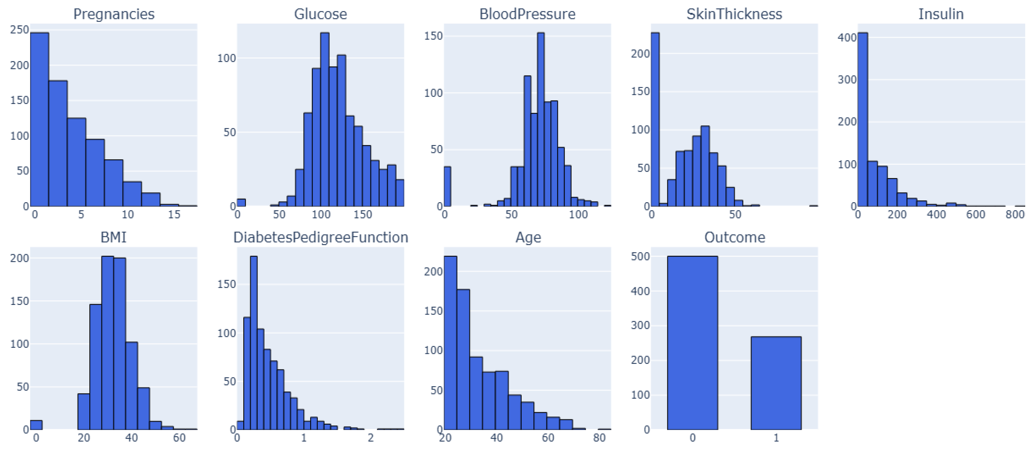
This is the PIMA Indian Diabetes dataset called Dataset 1. It has 768 samples and nine features, including clinical measures and patient characteristics. The dataset features are Pregnancy, Blood Pressure, Insulin, Skin Thickness, BMI, Diabetes Pedigree-Function, Age, and Outcome. The dataset contains no duplicate entries or missing values (NaNs); all characteristics are numerical. However, several features, especially those related to blood pressure, skin thickness, insulin, glucose, and BMI, contain sundry zero values, which is biologically impossible. Section 3.3 will discuss these discrepancies and their ramifications [72,73,74,75,76].
3.4.2. Dataset 2
This is also PIMA Indian Diabetes dataset, henceforth referred to as Dataset 2. It also has numerical characteristics about clinical measures and patient demographics and is structured similarly to Dataset 1. However, it is much larger with 2000 samples rather than 768 but 9 features.
3.4.3. Dataset 3
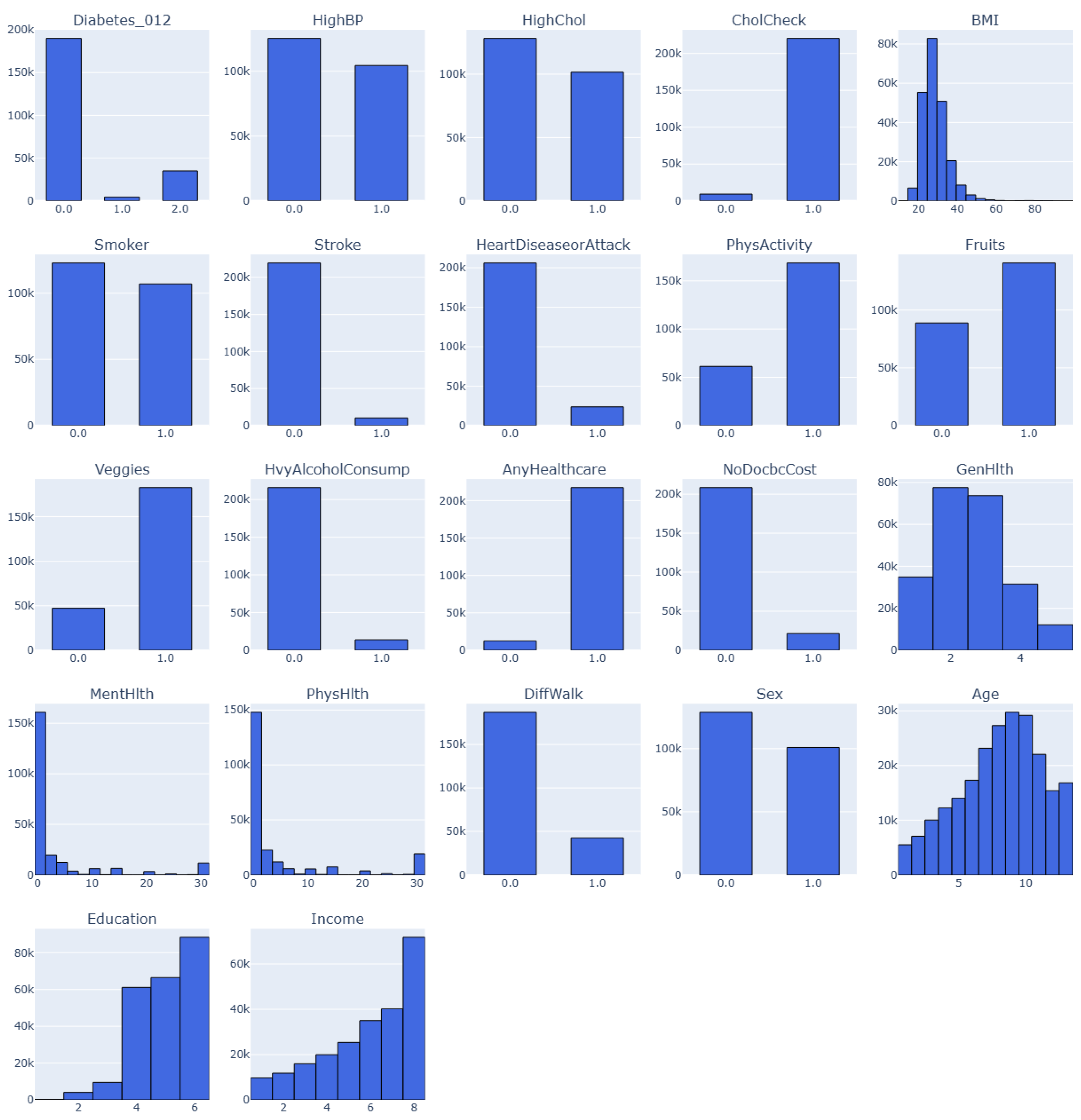
This is an annual Behaviorual Risk Factor Surveillance System (BRFSS) dataset captured by the Center for Disease Control (CDC). This dataset is for the year 2015. Henceforth, the dataset would be known as Dataset 3. The target variable has three classes (0, 1, 2). 0 is for no diabetes or only during pregnancy, 1 is for prediabetes, and 2 is for diabetes. There is a class imbalance in the dataset, but it has 21 features and 253,680 samples [77]
Figure 1.
Feature Distribution for Dataset 1 and Dataset 2 (PIMA dataset).
3.4.4. Dataset 4
This variant of Dataset 3 consists of 253,680 samples and 21 features of the BRFSS dataset captured by CDC for 2015. Here, the target consists of two classes (0, 1). 0 is for no diabetes, and 1 is for prediabetes or diabetes. It also contains class imbalance and would be known as Dataset 4 in this study.
Figure 2.
Feature Distribution for Dataset 3 and Dataset 4 (BRFSS_2015 dataset). .
3.4.5. Dataset 5
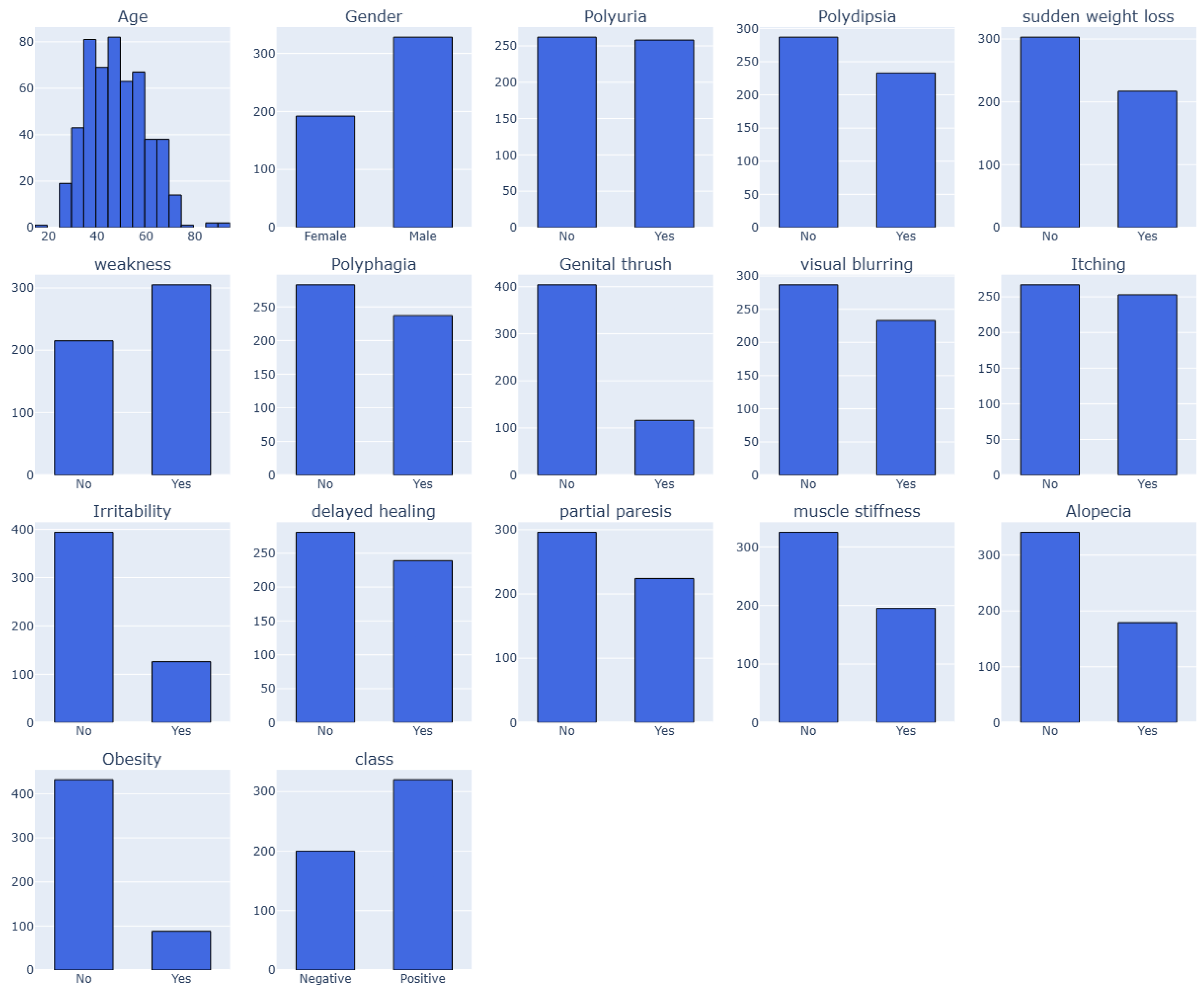
The early-stage diabetes risk prediction of patients from Sylhet Diabetes Hospital, Bangladesh, were captured in this dataset. Direct surveys from the patients were used in the study [78]. This dataset report includes 520 people with diabetes-related symptoms and information on people who may have diabetes-related symptoms. The dataset has 520 cases and 17 features, including the target class. A certified physician from Sylhet Diabetes Hospital verified the dataset, collected in 2020. The dataset, which includes several categorical (Yes/No) variables associated with diabetes diagnosis, is displayed in Appendix A. The "Class" property indicates the patient's diabetes status as either positive (1) or negative (2). The values of 1 (yes) or 2 (no) for each feature indicate whether the associated symptom or condition is present. However, there are four categories for the "Age" attribute: 1 for those aged 20–35, 2 for those aged 36–45, 3 for those aged 46–55, 4 for those aged 56–65 and 5 for those aged above 65. These characteristics and values serve as the foundation for developing a classification algorithm that uses patient data to forecast the diagnosis of diabetes [79,80].
Figure 3.
Feature Distribution for Dataset 5 (BRFSS_2015 dataset).
3.5. Preprocessing
Improving model accuracy and dependability through preprocessing datasets is essential in getting raw data ready for ML. Cleaning to deal with outliers and missing values, data transformation through standardization or normalization, and categorical feature conversion using one-hot encoding is usually part of it. Different dimensionality reduction techniques aid in the management of big feature collections. Sampling techniques such as SMOTE can be used to rectify class imbalance. Hence, to properly assess this study model performance, the five datasets are divided into ratio 80:20 subsets for the training and testing/validation process. In addition to lowering computing complexity and improving the prediction ability of ML models, proper preprocessing guarantees the dataset's quality.
Performing the exploratory data analysis (EDA) of each dataset, it was observed that zero values exist in columns where they are not physiologically conceivable, which is a significant problem in both Datasets 1 and 2. Missing data may be entered as zeros instead of NaN, resulting in inaccurate numbers. Table 1 shows zero values concerning affected features under Datasets 1 and 2.
Two imputation techniques are employed to deal with the problem of zero values in columns such as BMI, Insulin, Glucose, Blood Pressure, and Skin Thickness) is biologically impossible:
- Median Imputation: In each column, the median of non-zero values for zeros is substituted.
- Minimum Imputation: Instead of actual measurement, the zeros may mean data was not collected. This might indicate that the physiological levels of the patients with missing results were normal. Consequently, we used each column's smallest non-zero value to impute missing data.
Remarkably, models trained using minimum imputation on the datasets consistently performed better than those trained with median imputation. This validates our prediction that missing data were likely connected with patients having normal measures rather than abnormal or severe results. Given that various imputation techniques can substantially influence model performance, this conclusion implies that comprehending the nature of missing data is essential in medical datasets.
The imbalance in the target variable, where one class was noticeably underrepresented, provided another difficulty for us while analyzing all datasets. From the outcome class in Table 2, Dataset 1 has 400 entries of 0(No) values and 214 entries of 1(Yes) values, while dataset 2 shows 1053 entries for a 0(No) values and 547 entries for a 1(Yes) value. The study concentrated on oversampling approaches to balance the dataset because undersampling was impractical given the already small quantity of data points. The study experimented with various oversampling techniques, such as ADASYN, SMOTE-ENN, random oversampling, and SMOTE. In overall, ADASYN produced the most significant outcomes out of all of these. ADASYN, like SMOTE, generates synthetic samples near the decision border, to improve minority class categorization. Thus, selecting the appropriate data balancing strategy is important as it impacts model performance.
Datasets 3 and 4 had considerable data points and were unbalanced, but Datasets 1 and 2 had fewer data points, as shown in Table 2. We thus used undersampling to the datasets to lessen this problem. Instead of random undersampling, we employed clustering-based undersampling on datasets 3 and 4, which maintains the underlying data distribution. Clustering-based undersampling chooses representative samples from each cluster, guaranteeing that important patterns and class features are preserved, in contrast to conventional techniques that randomly exclude data points. It keeps crucial information from being lost despite its high computational cost.
Simple binary encoding was used to transform (encode) categorical characteristics into numerical representations to guarantee consistency across all datasets. To normalize the data and guarantee that each feature had a similar range, feature scaling was also used. This step is essential for optimising ML models because it keeps characteristics with bigger magnitudes from overpowering those with smaller values.
Because of the considerable class imbalance, where the dominant class significantly outnumbered the minority class, the experimental assessment showed that modelling Datasets 3 and 4 presented significant obstacles. As demonstrated by the models' total incapacity to detect any occurrences of the minority class, this extreme imbalance ratio made it difficult to create useful prediction models. Despite the thorough use of a variety of sampling strategies, including undersampling techniques like cluster centroids, Tomek links, and random undersampling for the majority class and oversampling techniques like SMOTE, ADASYN, and random oversampling for the minority class, the failure persisted. This is essentially based on the size of the datasets and the corresponding features.
4. Results Analysis
The results demonstrate the outcomes of a comprehensive investigation by using comparison tables, confusion matrices, density graphs and informative bar charts across all models used. Python programming language platform was used to implement all these processes. The model training procedure was systematically conducted for each model, following an encoded sequence of features. The datasets were split into training and testing groups. The training process was managed using the X_train and y_train values. The performance of the models was recorded by generating the predictions on the test datasets (X_test). In contrast, the efficiency of the models was accessed by evaluating their performance through metrics such as accuracy, precision, recall, F1-score, AUC-ROC, among others.
Confusion matrix and AUC-ROC visualization were also used in this study to gain detailed information on the performance of each model. This allowed for TP, TN, FP, and FN identification, while heatmaps visualization was presented to enhance the perception of performance complexities in these matrices. Graphs were used to visualize the outputs and comparisons, while the tables illustrate the values assigned to each model’s performance.
4.1. Result Analysis on Dataset 1
After performing a series of analysis on Dataset 1 (PIMA – 768/9) shown in Table 3 and Figure 4, Figure 5 demonstrate the analysis results, its corresponding confusion matrix, Precision/Recall and the AUC-ROC representation. The XGBoost model performed the best on this dataset, achieving an F1 score of 0.72.
4.2. Result Analysis on Dataset 2
Performance analysis on Dataset 2 (PIMA – 2000/9) shown in Table 4 and Figure 6 and Figure 7 demonstrate the analysis results, its corresponding confusion matrix, Precision/Recall and the AUC-ROC representation. The Decision Tree model performed the best on this dataset, achieving an F1 score of 0.98.
4.3. Result Analysis on Dataset 3
Performance analysis on Dataset 3 (BRFSS – 253,680 samples/21 features with three classes outcomes) are shown in Table 5, Figure 8, and Figure 9 demonstrate the results of the analysis, its corresponding confusion matrix, Precision/Recall and the AUC-ROC representation. The AdaBoost model performed better than other models on this dataset, achieving an F1 score of 0.43.
4.4. Result Analysis on Dataset 4
Performance analysis on Dataset 4 (BRFSS – 253,680 samples/21 features with two classes outcomes) shown in Table 6, Figure 10 and Figure 11 demonstrate the results of the analysis, its corresponding confusion matrix, Precision/Recall and the AUC-ROC representation. The logistic regression model performed better than other models on this dataset, achieving an F1 score of 0.44.
4.5. Result Analysis on Dataset 5
Performance analysis on Dataset 5 (early-stage diabetes risk prediction of patients of 520 samples and 17 features from Sylhet Diabetes Hospital, Bangladesh, shown in Table 7, Figure 12, and Figure 13 demonstrate the results of the analysis, its corresponding confusion matrix, Precision/Recall and the AUC-ROC representation. The Random Forest Tree, DT, and AdaBoost models performed the best on this dataset, achieving an F1 score of 0.9921 and a reasonable accuracy of 0.9904. RF is picked as the best of their best computation time in predicting diabetes in 0.0074s.
5. Discussion
Regarding both computational efficiency and predictive effectiveness, the experimental findings from all five datasets consistently show that classical machine learning models outperform deep learning techniques. These results address our study issues about processing time and model correctness based on the size of the datasets and the importance of the features concerning the datasets.
According to the analysis, tree-based models continuously strike the optimum balance between speed and accuracy. On Dataset 1, XGBoost performs best with an F1-score of 0.7244 and completes predictions in 0.0122 seconds, about 350 times quicker than similar hybrid models such as XGBoost-LSTM (11.4212s). Decision Trees demonstrate perfect recall (1.0000) on Dataset 2, while Random Forest achieves immaculate precision (1.0000) on Dataset 5, all while keeping prediction durations under a second. This trend is consistent across datasets.
Compared to their computing cost, deep learning models routinely perform poorly, which is evident based on the size of all the datasets that might not be adequate for DL models. Some neural network variations in need orders of magnitude demand more processing time, even when they attain competitive accuracy (within 2-3% of the top ML models). AdaBoost, for example, performs correspondingly results to XGBoost- CNN (F1 0.4314 vs 0.4271) on Dataset 3, but completes predictions three times quicker (19.4743s vs. 55.5742s). A distinct hierarchy in model efficiency is evident from the time measurements.
Across all datasets, traditional machine learning techniques (Decision Trees, Random Forest, XGBoost) consistently provide the quickest prediction speeds, usually less than a second. On Dataset 4, Logistic Regression is especially effective, obtaining a decent result (F1 0.4392) in just 0.2 seconds. On the other hand, DL models and hybrid techniques show noticeably higher processing times; for Dataset 4 predictions, some RNN variations take more than 1800 seconds to make their predictions. Nevertheless, Xie et al. [77] in their study proved that NN produces a better accuracy of 0.8240 but a lower recall of 0.3781. This is evident because the dataset size is inadequate for DL models.
According to the comparative analysis of Dataset 5, the results show ML models performing well across all metrics compared to DL models as reported by Xie et al. [78] even though both studies showed that RF outperformed other classical ML models. However, the analysis shows a value of 0.9740 across all metrics, while our study performed better using the same ML model with a value of 0.9921.
5.1. Comparative Analysis of Results with Already Developed Diabetes Prediction Models
The results analysed above compare the methods of ML and DL and their ensembles for predicting the health outcomes of diabetic patients. The generated outcomes must be compared with other models and existing developed predictive models based on the datasets used in this study (i.e. Datasets 1 – 5 ). It was observed that ML models demonstrated excellent accuracy and computation time with sufficient results, although this cannot be denied concerning the size of the datasets. However, the ML models presented good accuracy, speed, F1-score, AUC-ROC, and a reasonable computation time frame compared to DLs and ensembles, as well as some existing predictive models based on the same samples and features. Table 8 presents a comparative analysis of the results of the models for datasets and existing predictive models.
6. Conclusions
In this study, we used five publicly accessible datasets to compare different machine learning, deep learning, and ensemble algorithms and their modifications in the context of predicting the health outcomes of diabetic patients. The outcome of the analysis was also compared with existing predictive models. The results showed that ML models were consistently superior to alternative DL and ensemble techniques, demonstrating their efficacy in correctly predicting DM illnesses across various datasets considering accuracy, reliability, processing time and computational efficiency. ML models demonstrated their promise as a robust and dependable approach by achieving notable accuracy, recall, and F1-score with strong AUC-ROC scores on almost all five datasets. However, given the scale of the datasets, these performances of DL and ensemble models might not be disregarded. Nevertheless, RF, DT, AdaBoost, LR, k-NN, and XGBoost performed well, while other classifiers in ML, DL, and ensemble performed to their capacity, depending on size. However, ensemble models, including XGBoost-CNN, RF-CNN, RF-GRU, and XGBoost-LSTM, also showed exceptional performance across all five datasets.
People of all ages are becoming more susceptible to diabetes. The current study showed that early diabetes identification might be crucial for treatment and enhanced health outcomes for individuals with the disease. Obesity may be prevented by taking easy awareness-raising steps like eating a low-sugar diet, exercising frequently, and leading a healthy lifestyle. Its relevance in healthcare is apparent since models and its ensembles show increasing promise in predicting diabetes and eventually lowering treatment costs and increasing computing efficiency. Finding the optimal model for predicting datasets created for diabetes progression and risk prediction is the primary contribution of this work.
We discovered that the ML models had the best accuracy and better computing cost. Lastly, using the same dataset, a comparison of the models with current predictive models showed how important it is to improve the health outcomes for diabetes patients. The ML models in this study performed better than the existing predictive models in terms of accuracy, F1-score, and recall. Nonetheless, this study may be updated often with a more complete dataset and additional examples, and it can include other commonly used methods for prediction.
There are not many restrictions on our study, though we could not prove causation since some datasets were cross-sectional, particularly the health risk indicators (Datasets 3 and 4) and Dataset 5 (BRFSS_2015) data, and the biological entries were inaccurate. Another drawback of the Dataset 5 data was that it was self-reported and hence susceptible to memory biases, which may impact how well our prediction models performed. Nonetheless, our prediction algorithms could be more effective in forecasting the health outcomes of diabetes patients now that clinical data and biomarkers are available.
Author Contributions
Conceptualization, methodology, software, validation, formal analysis, investigation, resources, data curation, writing—original draft preparation, O.B.A.; writing—review and editing, visualization, supervision, project administration, S.S., C.R.; funding acquisition, S.S., O.B.A.
Funding
This research was funded by the Australian Research Training Program (RTP) Postgraduate Research Scholarship Award, and “The APC was funded by a waiver on my Principal Supervisor”. The Australian Government awarded the scholarship.
Data Availability Statement
All datasets used in this research are publicly available in Kaggle, CDC, and UCI Machine Learning Repository.
Acknowledgments
This work is part of the doctorate research under the Research Training Program (RTP) scholarship opportunity. The authors thank the anonymous reviewers for their valuable suggestions and comments on this paper.
Conflicts of Interest
The authors declare no conflicts of interest.
Abbreviations
| DM | Diabetes Mellitus |
| ML | Machine Learning |
| DL | Deep Learning |
| AU-ROC | Area under the ROC |
| KPI | Key Performance Indicators |
| IDF | International Diabetes Federation |
| T1DM | Type 1 DM |
| T2DM | Type 2 DM |
| GDM | Gestational DM |
| RF | Random Forest |
| LR | Logistic Regression |
| XGBoost | Extreme Gradient Boosting |
| NB | Naive Bayes |
| SVM | Support Vector Machine |
| NN | Neural Networks |
| RNN | Recurrent NN |
| CNN | Convolutional NN |
| DNN | Deep NN |
| QML | Quantum ML |
| KNN | k-Nearest Neighbour |
| CVD | Cardiovascular diseases |
| DT | Decision Tress |
| LSTM | Long Short-Term Memory |
| AdaBoost | Adaptive Boosting |
| GRU | Gated Recurrent Unit |
| ANN | Artificial Neural Networks |
Appendix A

Table A1.
Datasets Information.
| Datasets Statistics Description | Dataset 1 | Dataset 2 | Dataset 3 | Dataset 4 | Dataset 5 |
|---|---|---|---|---|---|
| Source | UCL Machine Learning Repository, Kaggle and CDC websites | ||||
| Samples | 768 | 2000 | 253,680 | 253,680 | 520 |
| Features | 9 | 9 | 21 | 21 | 17 |
| Positive instances | 268 | 684 | 35346 | 35346 | 320 |
| Negative instances | 500 | 1316 | 218334 | 35346 | 200 |
References
- Kavakiotis, O. Tsave, A. Salifoglou, N. Maglaveras, I. Vlahavas, and I. Chouvarda, "Machine Learning and Data Mining Methods in Diabetes Research," Computational and Structural Biotechnology Journal, vol. 15, pp. 104-116, 2017. [CrossRef]
- IDF, International Diabetes Federation (IDF) Diabetes Atlas 2021 (IDF Atlas 2021). 2021, pp. 1-141.
- M. A. R. Refat, M. A. Amin, C. Kaushal, M. N. Yeasmin, and M. K. Islam, "A Comparative Analysis of Early Stage Diabetes Prediction using Machine Learning and Deep Learning Approach," in 6th IEEE International Conference on Signal Processing, Computing and Control (ISPCC), Solan, India, 2021 2021: IEEE, pp. 654-659. [Online]. Available: https://ieeexplore.ieee.org/document/9609364/. [CrossRef]
- S. Ayon and M. M. Islam, "Diabetes Prediction: A Deep Learning Approach," International Journal of Information Engineering and Electronic Business, vol. 11, no. 2, pp. 21-27, 2019. [CrossRef]
- U. M. Butt et al., "Machine Learning Based Diabetes Classification and Prediction for Healthcare Applications," Journal of Healthcare Engineering, vol. 2021, pp. 9930985-17, 2021. [CrossRef]
- S. Alex David et al., "Comparative Analysis of Diabetes Prediction Using Machine Learning," in Soft Computing for Security Applications, vol. 1428, G. Ranganathan, X. Fernando, and S. Piramuthu Eds., (Advances in Intelligent Systems and Computing. Singapore: Springer, 2022, ch. 13, pp. 155-163.
- E. Longato, G. P. Fadini, G. Sparacino, A. Avogaro, L. Tramontan, and B. Di Camillo, "A Deep Learning Approach to Predict Diabetes' Cardiovascular Complications From Administrative Claims," IEEE journal of biomedical and health informatics, vol. 25, no. 9, pp. 3608-3617, 2021. [CrossRef]
- P. Saeedi et al., "Global and regional diabetes prevalence estimates for 2019 and projections for 2030 and 2045: Results from the International Diabetes Federation Diabetes Atlas, 9(th) edition," Diabetes Res Clin Pract, vol. 157, p. 107843, Nov 2019. [CrossRef]
- K. Zarkogianni, M. Athanasiou, A. C. Thanopoulou, and K. S. Nikita, "Comparison of Machine Learning Approaches Toward Assessing the Risk of Developing Cardiovascular Disease as a Long-Term Diabetes Complication," IEEE Journal of Biomedical and Health Informatics, vol. 22, no. 5, pp. 1637-1647, 2018. [CrossRef]
- Dinh, S. Miertschin, A. Young, and S. D. Mohanty, "A data-driven approach to predicting diabetes and cardiovascular disease with machine learning," BMC Med Inform Decis Mak, vol. 19, no. 1, p. 211, Nov 6 2019. [CrossRef]
- M. M. Hasan et al., "Cardiovascular Disease Prediction Through Comparative Analysis of Machine Learning Models," presented at the 2023 International Conference on Modeling & E-Information Research, Artificial Learning and Digital Applications (ICMERALDA), Karawang, Indonesia, 24-24 November 2023, 2023.
- X. Lin et al., "Global, regional, and national burden and trend of diabetes in 195 countries and territories - an analysis from 1990 to 2025," Sci Rep, vol. 10, no. 1, 14790, pp. 1-11, 2020. [CrossRef]
- S. Kodama et al., "Predictive ability of current machine learning algorithms for type 2 diabetes mellitus: A meta-analysis," J Diabetes Investig, vol. 13, no. 5, pp. 900-908, May 2022. [CrossRef]
- S. Larabi-Marie-Sainte, L. Aburahmah, R. Almohaini, and T. Saba, "Current Techniques for Diabetes Prediction: Review and Case Study," Applied sciences, vol. 9, no. 21, p. 4604, 2019. [CrossRef]
- S. Islam and F. Tariq, "Machine Learning-Enabled Detection and Management of Diabetes Mellitus," in Artificial Intelligence for Disease Diagnosis and Prognosis in Smart Healthcare, 2023, pp. 203-218.
- E. Afsaneh, A. Sharifdini, H. Ghazzaghi, and M. Z. Ghobadi, "Recent applications of machine learning and deep learning models in the prediction, diagnosis, and management of diabetes: a comprehensive review," Diabetol Metab Syndr, vol. 14, no. 1, p. 196, Dec 27 2022. [CrossRef]
- C. Giacomo, V. Martina, S. Giovanni, and F. Andrea, "Continuous Glucose Monitoring Sensors for Diabetes Management - A Review of Technologies and Applications," Diabetes Metabolism Journal, vol. 43, pp. 383-397, 2019. [CrossRef]
- Nomura, M. Noguchi, M. Kometani, K. Furukawa, and T. Yoneda, "Artificial Intelligence in Current Diabetes Management and Prediction," Curr Diab Rep, vol. 21, no. 12, p. 61, Dec 13 2021. [CrossRef]
- Z. Guan et al., "Artificial intelligence in diabetes management: Advancements, opportunities, and challenges," Cell Rep Med, vol. 4, no. 10, p. 101213, Oct 17 2023. [CrossRef]
- H. Y. Lu et al., "Digital Health and Machine Learning Technologies for Blood Glucose Monitoring and Management of Gestational Diabetes," IEEE Rev Biomed Eng, vol. 17, pp. 98-117, 2024. [CrossRef]
- T. Ba, S. Li, and Y. Wei, "A data-driven machine learning integrated wearable medical sensor framework for elderly care service," Measurement, vol. 167, 2021. [CrossRef]
- J. Kakoly, M. R. Hoque, and N. Hasan, "Data-Driven Diabetes Risk Factor Prediction Using Machine Learning Algorithms with Feature Selection Technique," Sustainability (Basel, Switzerland), vol. 15, no. 6, pp. 1-15, 2023, Art no. 4930. [CrossRef]
- T. Mora, D. Roche, and B. Rodriguez-Sanchez, "Predicting the onset of diabetes-related complications after a diabetes diagnosis with machine learning algorithms," Diabetes Res Clin Pract, vol. 204, pp. 1-7, Oct 2023. [CrossRef]
- B. C. Han, J. Kim, and J. Choi, "Prediction of complications in diabetes mellitus using machine learning models with transplanted topic model features," Biomedical engineering letters, vol. 14, no. 1, pp. 163-171, 2024. [CrossRef]
- Dagliati et al., "Machine Learning Methods to Predict Diabetes Complications," Journal of Diabetes Science and Technology, vol. 12, no. 2, pp. 295-302, 2018. [CrossRef]
- D. Ochocinski et al., "Life-Threatening Infectious Complications in Sickle Cell Disease: A Concise Narrative Review," Front Pediatr, vol. 8, p. 38, 2020. [CrossRef]
- K. R. Tan et al., "Evaluation of Machine Learning Methods Developed for Prediction of Diabetes Complications: A Systematic Review," Journal of Diabetes Science and Technology, vol. 17, no. 2, pp. 474-489, 2023. [CrossRef]
- S. Chauhan, M. S. Varre, K. Izuora, M. B. Trabia, and J. S. Dufek, "Prediction of Diabetes Mellitus Progression Using Supervised Machine Learning," Sensors (Basel), vol. 23, no. 10, May 11 2023. [CrossRef]
- J. S. Skyler et al., "Differentiation of Diabetes by Pathophysiology, Natural History, and Prognosis," Diabetes, vol. 66, no. 2, pp. 241-255, 2017. [CrossRef]
- M. Z. Banday, A. S. Sameer, and S. Nissar, "Pathophysiology of diabetes - An overview," Avicenna Journal of Medicine, vol. 10, no. 4, pp. 174–188, 2020. [CrossRef]
- W. Y. Fujimoto, "The Importance of Insulin Resistance in the Pathogenesis of Type 2 Diabetes Mellitus," American Journal of Medicine, vol. 108, 6A, pp. 9S-14S, 2000. [CrossRef]
- U. Galicia-Garcia et al., "Pathophysiology of Type 2 Diabetes Mellitus," International Journal of Molecular Science, vol. 21, no. 17, 2020. [CrossRef]
- Agliata, D. Giordano, F. Bardozzo, S. Bottiglieri, A. Facchiano, and R. Tagliaferri, "Machine Learning as a Support for the Diagnosis of Type 2 Diabetes," Int J Mol Sci, vol. 24, no. 7, pp. 1-14, Apr 5 2023, Art no. 6775. [CrossRef]
- H. D. McIntyre, P. Catalano, C. Zhang, G. Desoye, E. R. Mathiesen, and P. Damm, "Gestational diabetes mellitus," Nature Reviews. Disease Primers, vol. 5, no. 1, pp. 1-19, 2019, Art no. 47. [CrossRef]
- J. F. Plows, J. L. Stanley, P. N. Baker, C. M. Reynolds, and M. H. Vickers, "The Pathophysiology of Gestational Diabetes Mellitus," International Journal of Molecular Sciences, vol. 19, no. 11, pp. 1-21, 2018, Art no. 3342. [CrossRef]
- R. Ahmad, M. Narwaria, and M. Haque, "Gestational diabetes mellitus prevalence and progression to type 2 diabetes mellitus: A matter of global concern," Advances in Human Biology, vol. 13, no. 3, pp. 232-237, 2023. [CrossRef]
- P. Mahajan, S. Uddin, F. Hajati, M. A. Moni, and E. Gide, "A comparative evaluation of machine learning ensemble approaches for disease prediction using multiple datasets," Health and technology, vol. 14, no. 3, pp. 597-613, 2024. [CrossRef]
- L. Flores, R. M. Hernandez, L. H. Macatangay, S. M. G. Garcia, and J. R. Melo, "Comparative analysis in the prediction of early-stage diabetes using multiple machine learning techniques," Indonesian Journal of Electrical Engineering and Computer Science, vol. 32, no. 2, p. 887, 2023. [CrossRef]
- H. Gupta, H. Varshney, T. K. Sharma, N. Pachauri, and O. P. Verma, "Comparative performance analysis of quantum machine learning with deep learning for diabetes prediction," Complex & intelligent systems, vol. 8, no. 4, pp. 3073-3087, 2022. [CrossRef]
- N. Aggarwal, C. B. Basha, A. Arya, and N. Gupta, "A Comparative Analysis of Machine Leaming-Based Classifiers for Predicting Diabetes," presented at the 2023 International Conference on Advanced Computing & Communication Technologies (ICACCTech), Banur, India, 23-24 December 20, 2023.
- M. A. R. Refat, M. A. Amin, C. Kaushal, M. N. Yeasmin, and M. K. Islam, "A Comparative Analysis of Early Stage Diabetes Prediction using Machine Learning and Deep Learning Approach," in 6th IEEE International Conference on Signal Processing, Computing and Control (ISPCC 2k21), Solan, India, 2021 2021: IEEE, pp. 654-659. [Online]. Available: https://ieeexplore.ieee.org/stampPDF/getPDF.jsp?tp=&arnumber=9609364&ref=. [CrossRef]
- M. Swathy and K. Saruladha, "A comparative study of classification and prediction of Cardio-Vascular Diseases (CVD) using Machine Learning and Deep Learning techniques," ICT Express, vol. 8, no. 1, pp. 109-116, 2022. [CrossRef]
- L. Fregoso-Aparicio, J. Noguez, L. Montesinos, and J. A. Garcia-Garcia, "Machine learning and deep learning predictive models for type 2 diabetes: a systematic review," Diabetology and Metabolic Syndrome, vol. 13, no. 1, pp. 148-148, 2021. [CrossRef]
- S. Uddin, A. Khan, M. E. Hossain, and M. A. Moni, "Comparing different supervised machine learning algorithms for disease prediction," BMC Medical Informatics and Decision Making, vol. 19, no. 1, pp. 281-281, 2019. [CrossRef]
- H. Naz and S. Ahuja, "Deep learning approach for diabetes prediction using PIMA Indian dataset," Journal of Diabetes and Metabolic Disorders, vol. 19, no. 1, pp. 391-403, 2020. [CrossRef]
- M. K. Hasan, M. A. Alam, D. Das, E. Hossain, and M. Hasan, "Diabetes Prediction Using Ensembling of Different Machine Learning Classifiers," IEEE Access, vol. 8, pp. 76516-76531, 2020. [CrossRef]
- K. Sahoo, C. Pradhan, H. Das, M. Rout, H. Das, and J. K. Rout, "Performance Evaluation of Different Machine Learning Methods and Deep-Learning Based Convolutional Neural Network for Health Decision Making," in Nature Inspired Computing for Data Science, vol. 871, M. Rout, J. K. Rout, and H. Das Eds., (Studies in Computational Intelligence. Switzerland: Springer International Publishing AG, 2020, ch. Chapter 8, pp. 201-212.
- H. Lai, H. Huang, K. Keshavjee, A. Guergachi, and X. Gao, "Predictive models for diabetes mellitus using machine learning techniques," BMC Endocrine Disorders, vol. 19, no. 1, pp. 101-101, 2019. [CrossRef]
- D. Elreedy and A. F. Atiya, "A Comprehensive Analysis of Synthetic Minority Oversampling Technique (SMOTE) for handling class imbalance," Information Sciences, vol. 505, pp. 32-64, 2019. [CrossRef]
- T. Wongvorachan, S. He, and O. Bulut, "A Comparison of Undersampling, Oversampling, and SMOTE Methods for Dealing with Imbalanced Classification in Educational Data Mining," Information - MDPI, vol. 14, no. 1, 2023. [CrossRef]
- R. Kaur, R. Sharma, and M. K. Dhaliwal, "Evaluating Performance of SMOTE and ADASYNtoClassify Falls and Activities of Daily Living," in Proceedings of the 12th International Conference on Soft Computing for Problem Solving. SocProS 2023, Springer, Singapore, M. Pant, K. Deep, and A. Nagar, Eds., 2024, vol. 995: Springer, in Lecture Notes in Networks and Systems. [CrossRef]
- R. Panigrahi, L. Kumar, and S. K. Kuanar, "An Empirical Study to Investigate Different SMOTE Data Sampling Techniques for Improving Software Refactoring Prediction," in Neural Information Processing. ICONIP 2020. Communications in Computer and Information Science, vol. 1332, H. Yang, K. Pasupa, A. C. Leung, J. T. Kwok, J. H. Chan, and I. e. King Eds. Switzerland: Springer, Cham, 2020, pp. 23-31.
- H. Sahlaoui, E. A. A. Alaoui, S. Agoujil, and A. Nayyar, "An empirical assessment of smote variants techniques and interpretation methods in improving the accuracy and the interpretability of student performance models," Education and Information Technologies, vol. 29, no. 5, pp. 5447-5483, 2023. [CrossRef]
- H. Haibo, B. Yang, E. A. Garcia, and L. Shutao, "ADASYN: Adaptive synthetic sampling approach for imbalanced learning," presented at the 2008 IEEE International Joint Conference on Neural Networks (IEEE World Congress on Computational Intelligence), 2008.
- E. A. Elsoud et al., "Under Sampling Techniques for Handling Unbalanced Data with Various Imbalance Rates - A Comparative Study," International Journal of Advanced Computer Science and Applications (IJACSA), vol. 15, no. 8, pp. 1274-1284, 2024.
- M. Bach and A. Werner, "Improvement of Random Undersampling to Avoid Excessive Removal of Points from a Given Area of the Majority Class," in Computational Science – ICCS 2021 - 21st International Conference Krakow, Poland, June 16–18, 2021 Proceedings, Part III, Poland, M. Paszynski, D. Kranzlmüller, V. V. Krzhizhanovskaya, J. J. Dongarra, and P. M. Sloot, Eds., 2021, vol. 12744: Springer, Cham, in ICCS 2021. Lecture Notes in Computer Science, pp. 172-186. [CrossRef]
- G.Rekha, A. K. Tyagi, and V. K. Reddy, "Performance Analysis of Under-Sampling and Over-Sampling Techniques for Solving Class Imbalance Problem," International Conference on Sustainable Computing in Science, Technology & Management (SUSCOM-2019), pp. 1305-1315, Feb 26-28, 2019 2019.
- R. D. Joshi and C. K. Dhakal, "Predicting Type 2 Diabetes Using Logistic Regression and Machine Learning Approaches," International Journal of Environmental Research and Public Health, vol. 18, no. 14, pp. 1-17, 2021, Art no. 7346. [CrossRef]
- M. Maniruzzaman et al., "Accurate Diabetes Risk Stratification Using Machine Learning: Role of Missing Value and Outliers," J Med Syst, vol. 42, no. 5, p. 92, Apr 10 2018. [CrossRef]
- S. Mittal and Y. Hasija, "Applications of Deep Learning in Healthcare and Biomedicine," in Deep Learning Techniques for Biomedical and Health Informatics, vol. 68, S. Dash, B. R. Acharya, M. Mittal, A. Abraham, and A. Kelemen Eds. Switzerland: Springer International Publishing AG, 2019, ch. Chapter 4, pp. 57-78.
- Iyer, J. S, and R. Sumbaly, "Diagnosis of Diabetes Using Classification Mining Techniques," International journal of data mining & knowledge management process, vol. 5, no. 1, pp. 1-14, 2015. [CrossRef]
- S. Barik, S. Mohanty, S. Mohanty, and D. Singh, "Analysis of Prediction Accuracy of Diabetes Using Classifier and Hybrid Machine Learning Techniques," in Intelligent and Cloud Computing, D. Mishra, R. Buyya, P. Mohapatra, and S. Patnaik Eds., (Smart Innovation, Systems and Technologies. Singapore: Springer Singapore, 2020, pp. 399-409.
- S. M. Ganie, M. B. Malik, and T. Arif, "Performance analysis and prediction of type 2 diabetes mellitus based on lifestyle data using machine learning approaches," Journal of Diabetes and Metabolic Disorders, vol. 21, no. 1, pp. 339-352, 2022. [CrossRef]
- Iparraguirre-Villanueva, K. Espinola-Linares, R. O. Flores Castaneda, and M. Cabanillas-Carbonell, "Application of Machine Learning Models for Early Detection and Accurate Classification of Type 2 Diabetes," Diagnostics (Basel), vol. 13, no. 14, Jul 15 2023. [CrossRef]
- Altamimi et al., "An automated approach to predict diabetic patients using KNN imputation and effective data mining techniques," BMC Medical Research Methodology, vol. 24, no. 1, 2024. [CrossRef]
- S. Suriya and J. J. Muthu, "Type 2 Diabetes Prediction using K-Nearest Neighbor Algorithm," Journal of Trends in Computer Science and Smart Technology, vol. 5, no. 2, pp. 190-205, 2023. [CrossRef]
- S. S. Salam and R. Rafi, "Deep Learning Approach for Sleep Apnea Detection Using Single Lead ECG: Comparative Analysis Between CNN and SNN," presented at the 2023 26th International Conference on Computer and Information Technology (ICCIT), Cox’s Bazar, Bangladesh, 13-15 December 2023, 2023.
- M. Rahman, D. Islam, R. J. Mukti, and I. Saha, "A deep learning approach based on convolutional LSTM for detecting diabetes," Computational biology and chemistry, vol. 88, pp. 107329-107329, 2020. [CrossRef]
- M. K. P, S. P. R, N. R K, and A. K, "Type 2: Diabetes mellitus prediction using Deep Neural Networks classifier," International Journal of Cognitive Computing in Engineering, vol. 1, pp. 55-61, 2020. [CrossRef]
- M. Z. Wadghiri, A. Idri, T. E. Idrissi, and H. Hakkoum, "Ensemble blood glucose prediction in diabetes mellitus - A review," Computational and Structural Biotechnology Journal, vol. 147, 105674, pp. 1-25, 2022. [CrossRef]
- Y. Guan and T. Plotz, "Ensembles of Deep LSTM Learners for Activity Recognition using Wearables," ACM, vol. 0, pp. 1-28, 2017.
- M. Y. Shams, Z. Tarek, and A. M. Elshewey, "A novel RFE-GRU model for diabetes classification using PIMA Indian dataset," Sci Rep, vol. 15, no. 1, p. 982, Jan 6 2025. [CrossRef]
- M. Raquibul Hossain, M. J. Hossain, M. M. Rahman, and M. Manjur Alam, "Machine Learning Based Prediction and Insights of Diabetes Disease: Pima Indian and Frankfurt Datasets," Journal of Mechanics of Continua and Mathematical Sciences, vol. 20, no. 1, 2025. [CrossRef]
- Mousa, W. Mustafa, and R. B. Marqas, "A Comparative Study of Diabetes Detection Using The Pima Indian Diabetes Database," The Journal of University of Duhok, vol. 26, no. 2, pp. 277-288, 2023. [CrossRef]
- S. Zargar, A. Bhagat, T. A. Teli, and S. Sheikh, "Early Prediction of Diabetes Mellitus on Pima Dataset Using ML And DL Techniques," Journal of Army Engineering University of PLA, vol. 23, no. 1, pp. 230-249, 2023.
- V. Chang, J. Bailey, Q. A. Xu, and Z. Sun, "Pima Indians diabetes mellitus classification based on machine learning (ML) algorithms," Neural Comput Appl, pp. 1-17, Mar 24 2022. [CrossRef]
- Z. Xie, O. Nikolayeva, J. Luo, and D. Li, "Building Risk Prediction Models for Type 2 Diabetes Using Machine Learning Techniques," Prev Chronic Dis, vol. 16, p. E130, Sep 19 2019. [CrossRef]
- M. M. F. Islam, R. Ferdousi, S. Rahman, and H. Y. Bushra, "Likelihood Prediction of Diabetes at Early Stage Using Data Mining Techniques," in Computer Vision and Machine Intelligence in Medical Image Analysis, (Advances in Intelligent Systems and Computing, 2020, ch. Chapter 12, pp. 113-125.
- Sadhu and A. Jadli, "Early-Stage Diabetes Risk Prediction - A Comparative Analysis of Classification Algorithms," International Advanced Research Journal in Science, Engineering and Technology, vol. 8, no. 1, pp. 193-201, 2021. [CrossRef]
- Q. A. Al-Haija, M. Smadi, and O. M. Al-Bataineh, "Early Stage Diabetes Risk Prediction via Machine Learning," Proceedings of the 13th International Conference on Soft Computing and Pattern Recognition (SoCPaR 2021), vol. 417, pp. 451-461, 2022. [CrossRef]
- S. P. Chatrati et al., "Smart home health monitoring system for predicting type 2 diabetes and hypertension," Journal of King Saud University - Computer and Information Sciences, vol. 34, no. 3, pp. 862-870, 2022. [CrossRef]
- M. R. Bozkurt, N. Yurtay, Z. Yilmaz, and C. Sertkaya, "Comparison of different methods for determining diabetes," Turkish Journal of Electrical Engineering & Computer Sciences, vol. 22, pp. 1044-1055, 2014. [CrossRef]
- S. Bashir, U. Qamar, and F. H. Khan, "IntelliHealth: A medical decision support application using a novel weighted multi-layer classifier ensemble framework," J Biomed Inform, vol. 59, pp. 185-200, Feb 2016. [CrossRef]
- Q. Wang, W. Cao, J. Guo, J. Ren, Y. Cheng, and D. N. Davis, "DMP_MI: An Effective Diabetes Mellitus Classification Algorithm on Imbalanced Data With Missing Values," IEEE Access, vol. 7, pp. 102232-102238, 2019. [CrossRef]
- H. Kaur and V. Kumari, "Predictive modelling and analytics for diabetes using a machine learning approach," Applied Computing and Informatics, vol. 18, no. 1/2, pp. 90-100, 2020. [CrossRef]
- N. Yuvaraj and K. R. SriPreethaa, "Diabetes prediction in healthcare systems using machine learning algorithms on Hadoop cluster," Cluster Computing, vol. 22, no. S1, pp. 1-9, 2017. [CrossRef]
Figure 4.
Confusion matrix for XGBoost model.
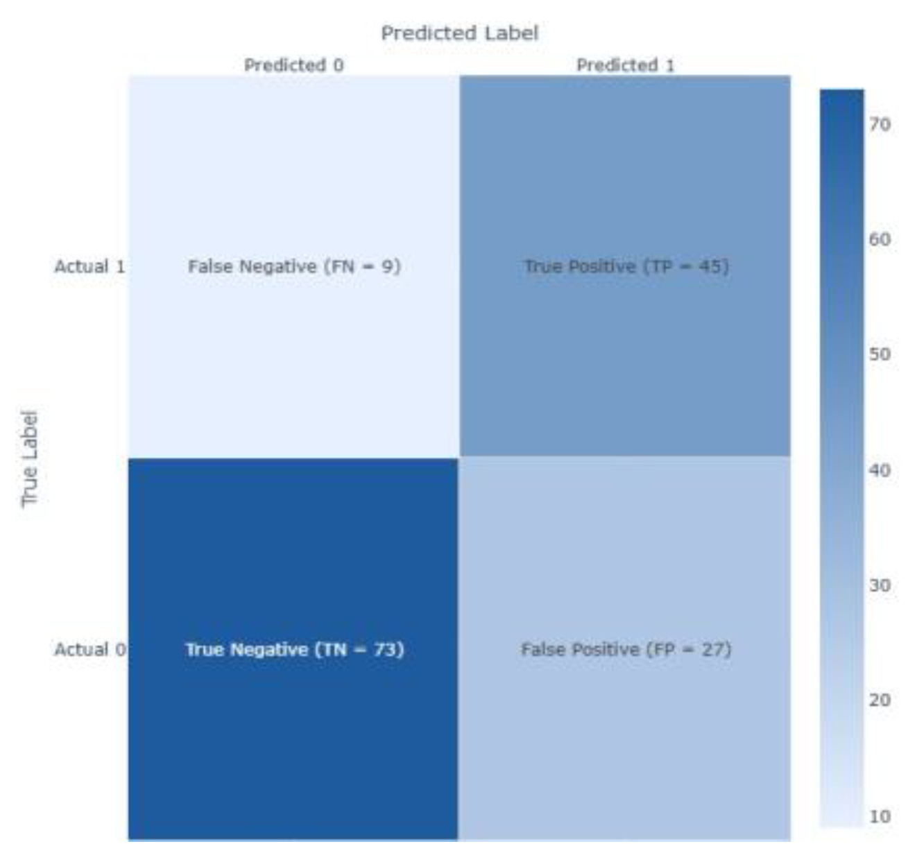
Figure 5.
AUC Curves for XGBoost model.

Figure 6.
Confusion matrix for Decision Tree model.
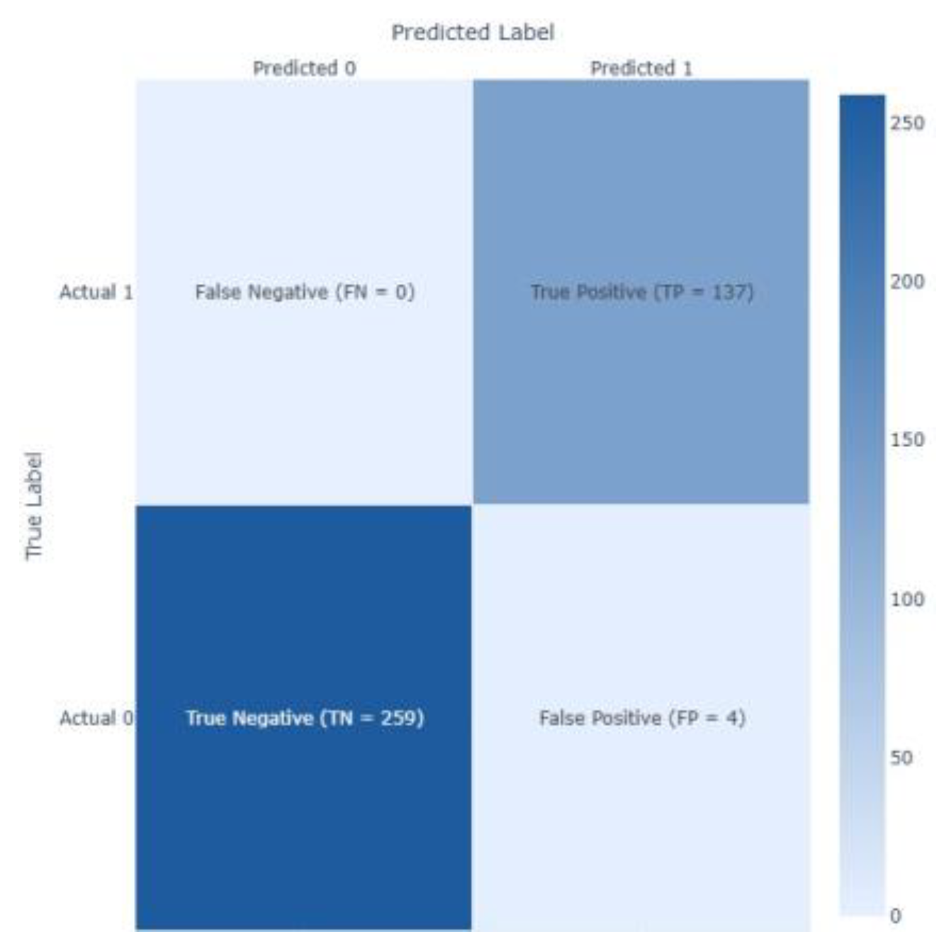
Figure 7.
AUC and Precision-Recall Curves for Decision Tree model.
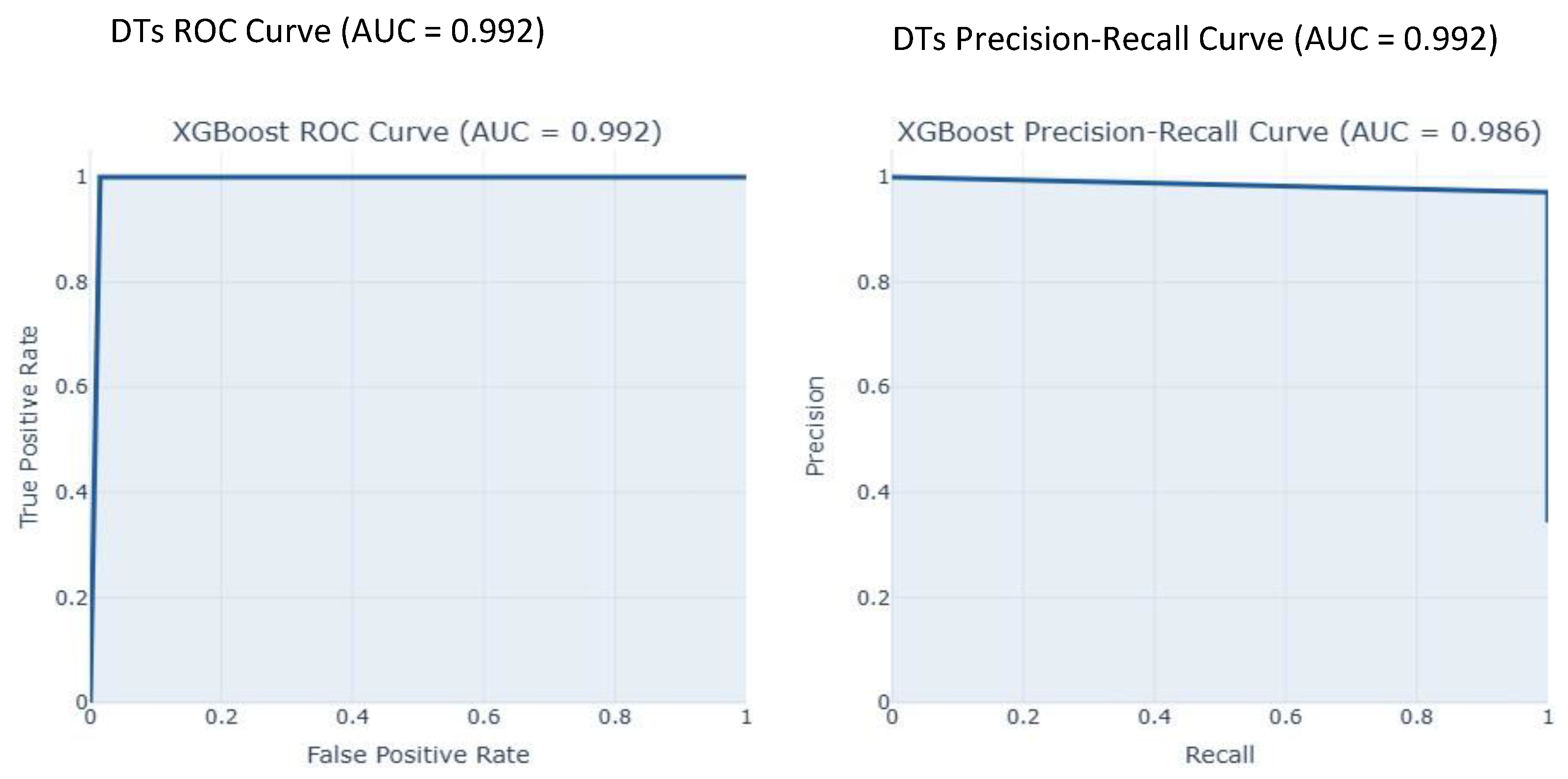
Figure 8.
Confusion matrix for the Logistic Regression model.
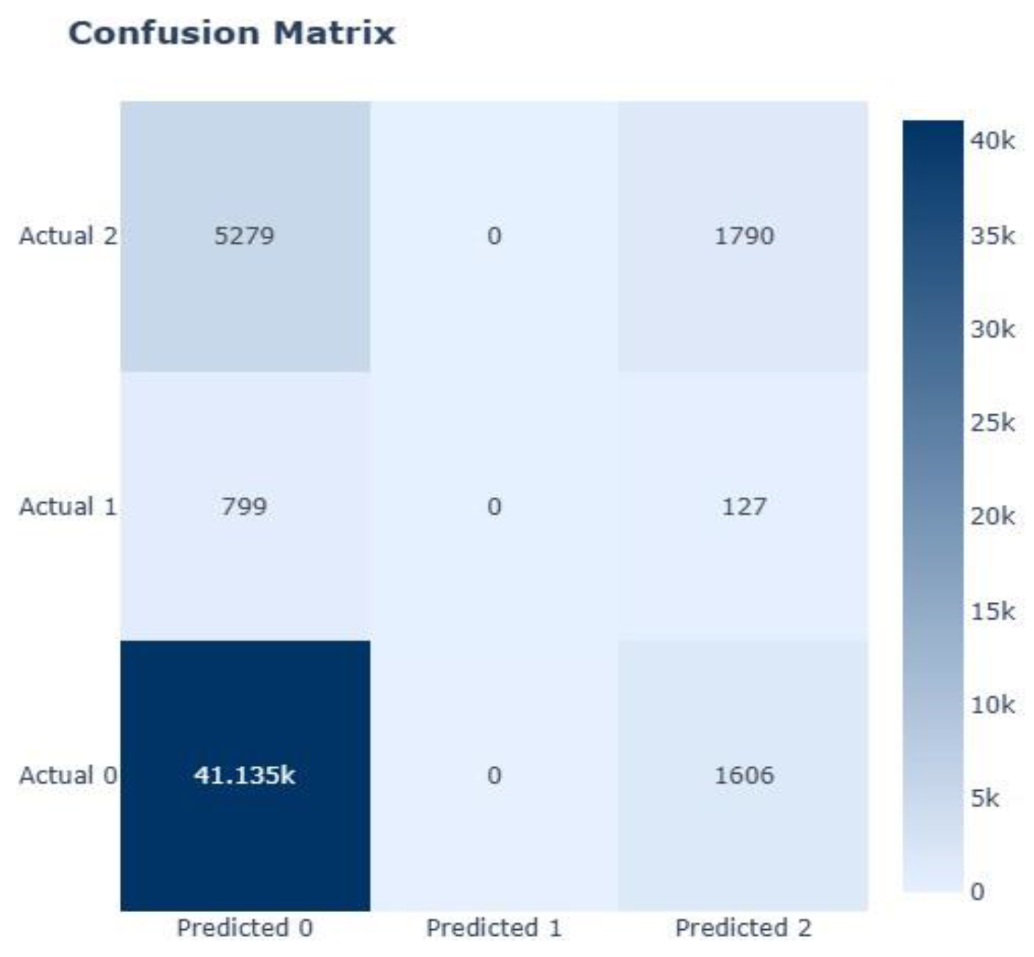
Figure 9.
AUC and Precision-Recall Curves of Logistic Regression Model.
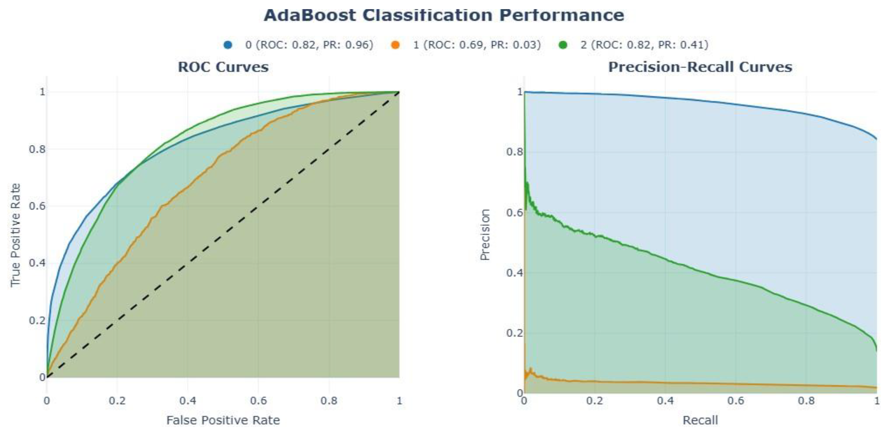
Figure 10.
Confusion matrix for the Logistic Regression model (Top). AUC Curves of Logistic Regression Model (bottom).
Figure 10.
Confusion matrix for the Logistic Regression model (Top). AUC Curves of Logistic Regression Model (bottom).
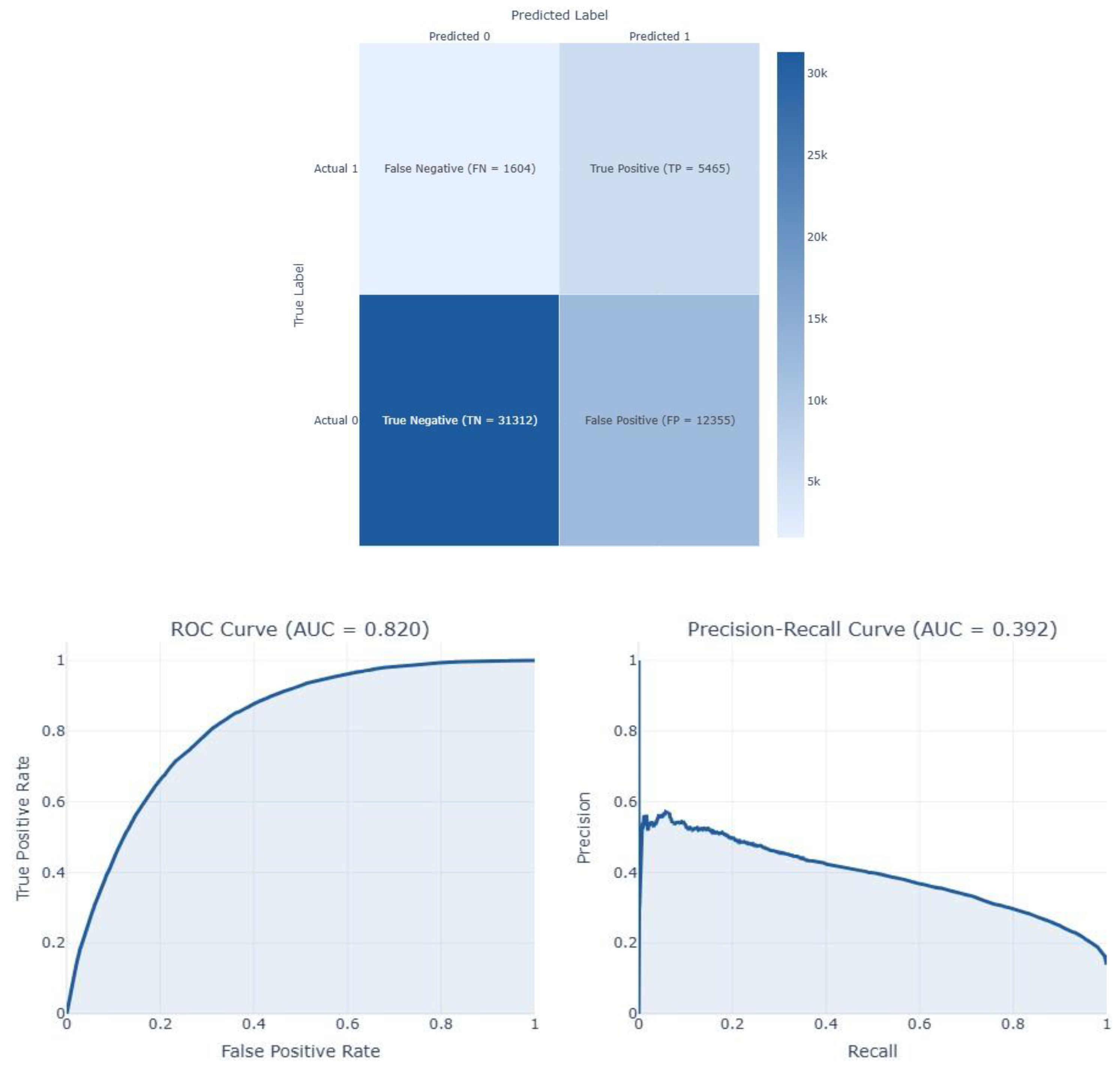
Figure 11.
Threshold-dependent metrics for LR. The vertical line denotes the chosen threshold.
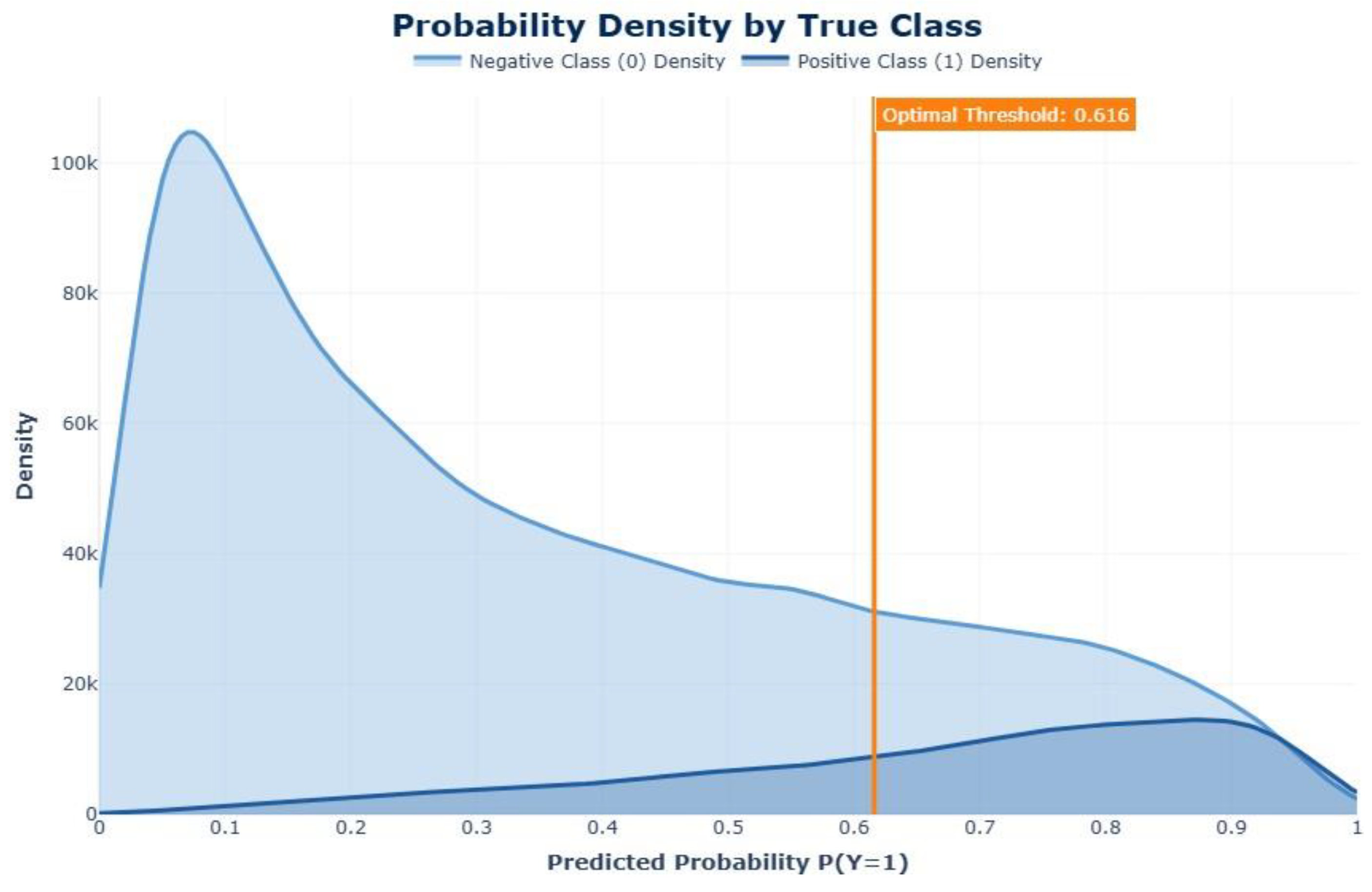
Figure 12.
Confusion matrix for Random Forest model.
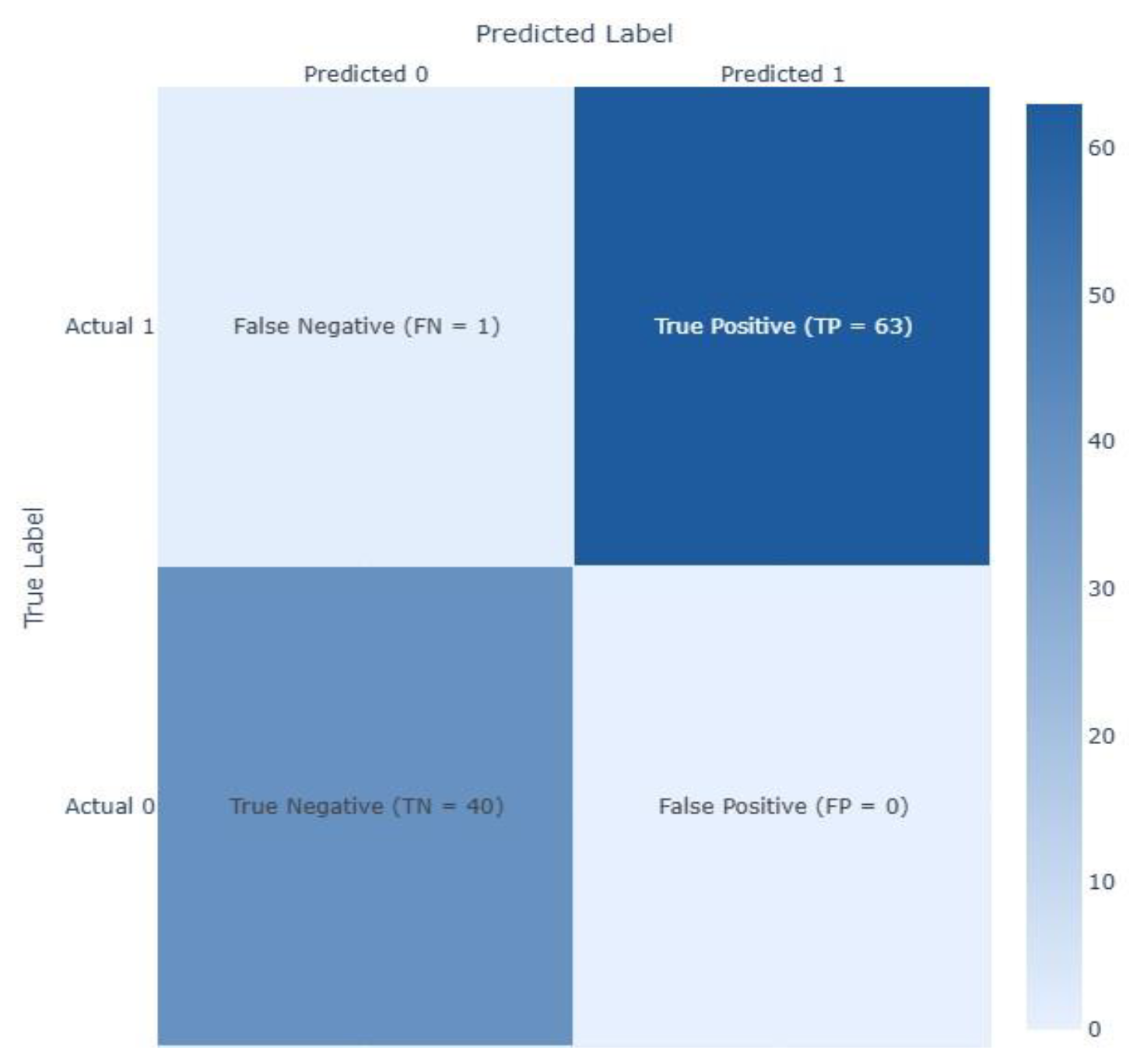
Figure 13.
AUC Curves for Random Forest model.
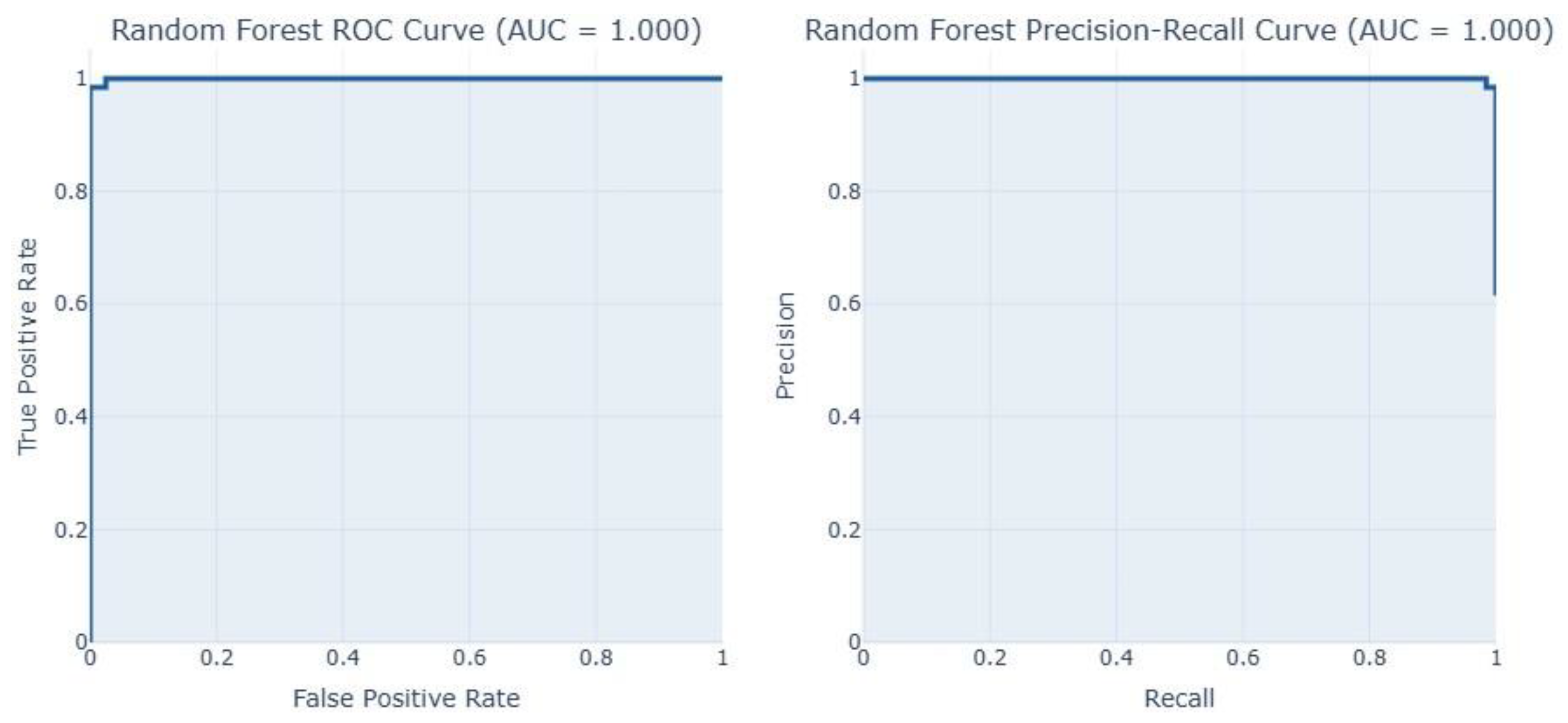
Table 1.
Number of data labelled as zero values.
| Feature | Dataset 1 | Dataset 2 |
|---|---|---|
| Pregnancies | 111 | 301 |
| Glucose | 5 | 13 |
| BloodPressure | 35 | 90 |
| SkinThickness | 227 | 573 |
| Insulin | 374 | 956 |
| BMI | 11 | 28 |
| DiabetesPedigreeFunction | 0 | 0 |
| Age | 0 | 0 |
Table 2.
Imbalance values in the Outcome (Target) variable.
| Outcome (Target class) | Dataset 1 | Dataset 2 | Dataset 3 | Dataset 4 | Dataset 5 |
|---|---|---|---|---|---|
| 0 | 400 | 1053 | 213703 | 218334 | 200 |
| 1 | 214 | 547 | 4631 | 35346 | 320 |
| 2 | - | - | 35346 | - | - |
Table 3.
Model Performance Comparison for Dataset 1 using F1-score as reference.
| Model | Accuracy | Precision | Recall | F1 Score | AUC-ROC | Time Taken (s) |
|---|---|---|---|---|---|---|
| XGBoost | 0.7727 | 0.6301 | 0.8519 | 0.7244 | 0.8356 | 0.0122 |
| XGBoost-CNN | 0.7727 | 0.6338 | 0.8333 | 0.7200 | 0.8224 | 4.3404 |
| AdaBoost | 0.7727 | 0.6338 | 0.8333 | 0.7200 | 0.8411 | 0.0091 |
| DNN | 0.7727 | 0.6377 | 0.8148 | 0.7154 | 0.8219 | 0.0144 |
| RF-GRU | 0.7597 | 0.6164 | 0.8333 | 0.7087 | 0.8120 | 9.1299 |
| Random Forest | 0.7597 | 0.6232 | 0.7963 | 0.6992 | 0.8196 | 0.0095 |
| Decision Tree | 0.7597 | 0.6308 | 0.7593 | 0.6891 | 0.7984 | 0.0167 |
| SVM | 0.7532 | 0.6176 | 0.7778 | 0.6885 | 0.8213 | 0.0145 |
| KNN | 0.7403 | 0.5946 | 0.8148 | 0.6875 | 0.8077 | 0.0147 |
| RF-CNN | 0.7597 | 0.6349 | 0.7407 | 0.6838 | 0.8120 | 0.0134 |
| Logistic Regression | 0.7468 | 0.6087 | 0.7778 | 0.6829 | 0.8189 | 0.0138 |
| LR-MLP | 0.7403 | 0.6029 | 0.7593 | 0.6721 | 0.8200 | 2.4844 |
| SVM-RNN | 0.7468 | 0.6119 | 0.7593 | 0.6777 | 0.8225 | 6.7487 |
| XGBoost-LSTM | 0.7403 | 0.6000 | 0.7778 | 0.6774 | 0.8219 | 11.4212 |
| DT-CNN | 0.6818 | 0.5275 | 0.8889 | 0.6621 | 0.7946 | 5.4317 |
| AdaBoost-DBN | 0.7013 | 0.5526 | 0.7778 | 0.6462 | 0.8004 | 18.8776 |
| CNN | 0.7143 | 0.5694 | 0.7593 | 0.6508 | 0.8219 | 0.0165 |
| KNN-Autoencoders | 0.6883 | 0.5417 | 0.7222 | 0.6190 | 0.7711 | 9.5224 |
| Naive Bayes | 0.6948 | 0.5522 | 0.6852 | 0.6116 | 0.7676 | 0.0908 |
| RNN | 0.6948 | 0.5522 | 0.6852 | 0.6116 | 0.7806 | 0.0110 |
| GRU | 0.6623 | 0.5156 | 0.6111 | 0.5593 | 0.7000 | 0.0106 |
| LSTM | 0.6688 | 0.5246 | 0.5926 | 0.5565 | 0.7013 | 0.0171 |
* All values are rounded to four decimal places.
Table 4.
Model Performance Comparison for Dataset 2 sing F1-score as reference.
| Model | Accuracy | Precision | Recall | F1 Score | AUC-ROC | Time Taken (s) |
|---|---|---|---|---|---|---|
| Decision Tree | 0.9900 | 0.9716 | 1.0000 | 0.9856 | 0.9924 | 0.0276 |
| Random Forest | 0.9850 | 0.9781 | 0.9781 | 0.9781 | 0.9972 | 0.0104 |
| KNN | 0.9850 | 0.9781 | 0.9781 | 0.9781 | 0.9942 | 0.0097 |
| AdaBoost | 0.9850 | 0.9781 | 0.9781 | 0.9781 | 0.9993 | 0.0091 |
| RF-CNN | 0.9850 | 0.9781 | 0.9781 | 0.9781 | 0.9972 | 0.0158 |
| XGBoost-LSTM | 0.9850 | 0.9781 | 0.9781 | 0.9781 | 0.9893 | 14.9132 |
| RF-GRU | 0.9850 | 0.9781 | 0.9781 | 0.9781 | 0.9958 | 9.6351 |
| XGBoost-CNN | 0.9850 | 0.9781 | 0.9781 | 0.9781 | 0.9888 | 6.3965 |
| DT-CNN | 0.9750 | 0.9504 | 0.9781 | 0.9640 | 0.9757 | 7.1950 |
| SVM-RNN | 0.9575 | 0.9167 | 0.9635 | 0.9395 | 0.9767 | 8.6150 |
| SVM | 0.9550 | 0.9103 | 0.9635 | 0.9362 | 0.9693 | 0.0136 |
| XGBoost | 0.9475 | 0.8867 | 0.9708 | 0.9268 | 0.9867 | 0.0107 |
| KNN-Autoencoders | 0.9125 | 0.8036 | 0.9854 | 0.8852 | 0.9871 | 21.7245 |
| AdaBoost-DBN | 0.8350 | 0.7052 | 0.8905 | 0.7871 | 0.9349 | 22.0284 |
| DNN | 0.8250 | 0.6872 | 0.8978 | 0.7785 | 0.9140 | 0.0123 |
| LR-MLP | 0.7975 | 0.6628 | 0.8321 | 0.7379 | 0.8891 | 11.9994 |
| CNN | 0.7800 | 0.6369 | 0.8321 | 0.7215 | 0.8590 | 0.0108 |
| RNN | 0.7600 | 0.6051 | 0.8613 | 0.7108 | 0.8549 | 0.0104 |
| Logistic Regression | 0.7600 | 0.6145 | 0.8029 | 0.6962 | 0.8524 | 0.0263 |
| GRU | 0.7400 | 0.5846 | 0.8321 | 0.6867 | 0.8467 | 0.0186 |
| Naive Bayes | 0.7525 | 0.6159 | 0.7372 | 0.6711 | 0.8322 | 0.0269 |
| LSTM | 0.7000 | 0.5464 | 0.7299 | 0.6250 | 0.7963 | 0.0240 |
* All values are rounded to four decimal places.
Table 5.
Model Performance Comparison for Dataset 3 using F1-score as reference.
| Model | Accuracy | Precision | Recall | F1 Score | AUC-ROC | Time Taken (s) |
|---|---|---|---|---|---|---|
| AdaBoost | 0.6973 | 0.4317 | 0.5122 | 0.4314 | 0.7103 | 19.4743 |
| XGBoost-CNN | 0.7018 | 0.4304 | 0.5088 | 0.4271 | 0.7167 | 55.5742 |
| XGBoost | 0.7044 | 0.4293 | 0.5068 | 0.4265 | 0.7137 | 6.0555 |
| RF-CNN | 0.6693 | 0.4314 | 0.5112 | 0.4249 | 0.7107 | 37.4420 |
| Random Forest | 0.6799 | 0.4274 | 0.5045 | 0.4244 | 0.6997 | 14.5153 |
| XGBoost-LSTM | 0.6936 | 0.4273 | 0.5049 | 0.4240 | 0.7094 | 198.5152 |
| RF-GRU | 0.6599 | 0.4328 | 0.5115 | 0.4230 | 0.7085 | 141.7040 |
| DT-CNN | 0.6890 | 0.4227 | 0.4783 | 0.4218 | 0.6566 | 43.6537 |
| Logistic Regression | 0.6259 | 0.4498 | 0.5154 | 0.4192 | 0.7077 | 3.2978 |
| GRU | 0.6678 | 0.4327 | 0.4752 | 0.4161 | 0.6729 | 210.8736 |
| DNN | 0.6428 | 0.4281 | 0.5109 | 0.4134 | 0.7052 | 51.4291 |
| LR-MLP | 0.5936 | 0.4561 | 0.5197 | 0.4117 | 0.7117 | 0.8947 |
| Decision Tree | 0.6329 | 0.4247 | 0.5028 | 0.4079 | 0.6878 | 0.2390 |
| Naive Bayes | 0.6245 | 0.4364 | 0.4892 | 0.4083 | 0.6803 | 0.1709 |
| CNN | 0.5787 | 0.4358 | 0.5180 | 0.3988 | 0.7037 | 69.0522 |
| SVM | 0.5775 | 0.4418 | 0.5012 | 0.3978 | 0.7005 | 453.5940 |
| KNN-Autoencoders | 0.5590 | 0.4116 | 0.4473 | 0.3650 | 0.6232 | 19.3189 |
| KNN (Normal) | 0.5327 | 0.4125 | 0.4476 | 0.3589 | 0.6251 | 25.1546 |
| AdaBoost-DBN | 0.5393 | 0.4414 | 0.4854 | 0.3806 | 0.6775 | 364.6265 |
| RNN | 0.5858 | 0.4197 | 0.4958 | 0.3878 | 0.6863 | 119.7845 |
| LSTM | 0.6769 | 0.4097 | 0.4746 | 0.4030 | 0.6728 | 278.3175 |
* All values are rounded to four decimal places.
Table 6.
Model Performance Comparison for Dataset 4 using F1-score as reference.
| Model | Accuracy | Precision | Recall | F1 Score | AUC-ROC | Time Taken (s) |
|---|---|---|---|---|---|---|
| Logistic Regression | 0.7249 | 0.3067 | 0.7731 | 0.4392 | 0.8197 | 0.2650 |
| LR-MLP | 0.7144 | 0.3017 | 0.7990 | 0.4381 | 0.8235 | 50.7898 |
| AdaBoost | 0.7251 | 0.3062 | 0.7690 | 0.4380 | 0.8187 | 2.0871 |
| XGBoost | 0.7132 | 0.3005 | 0.7971 | 0.4365 | 0.8209 | 0.9791 |
| XGBoost-CNN | 0.7079 | 0.2969 | 0.8010 | 0.4332 | 0.8212 | 58.5367 |
| GRU | 0.7111 | 0.2985 | 0.7947 | 0.4340 | 0.8187 | 217.5773 |
| CNN | 0.7044 | 0.2959 | 0.8131 | 0.4339 | 0.8238 | 53.9654 |
| XGBoost-LSTM | 0.7072 | 0.2960 | 0.7990 | 0.4320 | 0.8204 | 208.5252 |
| SVM-RNN | 0.7021 | 0.2943 | 0.8138 | 0.4322 | 0.8112 | 1804.6831 |
| RNN | 0.7047 | 0.2947 | 0.8037 | 0.4313 | 0.8184 | 113.6648 |
| DNN | 0.6872 | 0.2864 | 0.8345 | 0.4264 | 0.8229 | 53.0682 |
| RF-GRU | 0.7036 | 0.2919 | 0.7906 | 0.4263 | 0.8101 | 252.4819 |
| LSTM | 0.7043 | 0.2925 | 0.7911 | 0.4271 | 0.8149 | 203.2224 |
| Random Forest | 0.7025 | 0.2899 | 0.7833 | 0.4232 | 0.8070 | 9.8154 |
| RF-CNN | 0.7034 | 0.2911 | 0.7864 | 0.4249 | 0.8095 | 76.8140 |
| AdaBoost-DBN | 0.6859 | 0.2855 | 0.8345 | 0.4254 | 0.8221 | 58.1984 |
| SVM | 0.7002 | 0.2917 | 0.8068 | 0.4285 | 0.8162 | 1541.3782 |
| KNN-Autoencoders | 0.6753 | 0.2624 | 0.7349 | 0.3868 | 0.7566 | 85.9556 |
| KNN | 0.6751 | 0.2620 | 0.7333 | 0.3861 | 0.7563 | 38.4936 |
| Decision Tree | 0.6599 | 0.2391 | 0.6599 | 0.3510 | 0.6606 | 0.3532 |
| DT-CNN | 0.6649 | 0.2417 | 0.6571 | 0.3534 | 0.6618 | 62.1882 |
| Naive Bayes | 0.7235 | 0.2941 | 0.7029 | 0.4147 | 0.7799 | 0.0977 |
* All values are rounded to four decimal places.
Table 7.
Model Performance Comparison for Dataset 5 using F1-score as reference.
| Model | Accuracy | Precision | Recall | F1 Score | AUC-ROC | Time Taken (s) |
|---|---|---|---|---|---|---|
| Random Forest | 0.9904 | 1.0000 | 0.9844 | 0.9921 | 1.0000 | 0.0074 |
| Decision Tree | 0.9904 | 1.0000 | 0.9844 | 0.9921 | 0.9922 | 0.0299 |
| AdaBoost | 0.9904 | 1.0000 | 0.9844 | 0.9921 | 0.9992 | 0.0389 |
| SVM | 0.9808 | 0.9844 | 0.9844 | 0.9844 | 0.9977 | 0.0181 |
| SVM-RNN | 0.9808 | 0.9844 | 0.9844 | 0.9844 | 0.9984 | 6.6874 |
| RF-GRU | 0.9808 | 1.0000 | 0.9688 | 0.9841 | 1.0000 | 8.2692 |
| RF-CNN | 0.9808 | 1.0000 | 0.9688 | 0.9841 | 0.9992 | 0.0132 |
| XGBoost-LSTM | 0.9808 | 1.0000 | 0.9688 | 0.9841 | 1.0000 | 11.2858 |
| XGBoost-CNN | 0.9808 | 1.0000 | 0.9688 | 0.9841 | 0.9977 | 4.1041 |
| CNN | 0.9712 | 0.9841 | 0.9688 | 0.9764 | 0.9977 | 0.0132 |
| DT-CNN | 0.9712 | 0.9841 | 0.9688 | 0.9764 | 0.9826 | 5.6472 |
| LR-MLP | 0.9712 | 0.9841 | 0.9688 | 0.9764 | 0.9992 | 9.9053 |
| XGBoost | 0.9615 | 0.9688 | 0.9688 | 0.9688 | 0.9926 | 0.0244 |
| KNN-Autoencoders | 0.9615 | 1.0000 | 0.9375 | 0.9677 | 0.9828 | 8.6576 |
| DNN | 0.9615 | 0.9839 | 0.9531 | 0.9683 | 0.9988 | 0.0146 |
| RNN | 0.9615 | 0.9839 | 0.9531 | 0.9683 | 0.9918 | 0.0112 |
| Logistic Regression | 0.9519 | 1.0000 | 0.9219 | 0.9594 | 0.9914 | 0.0515 |
| KNN | 0.9519 | 0.9836 | 0.9375 | 0.9600 | 0.9633 | 0.0190 |
| Naive Bayes | 0.9423 | 0.9677 | 0.9375 | 0.9524 | 0.9863 | 0.0146 |
| AdaBoost-DBN | 0.9231 | 0.9828 | 0.8906 | 0.9344 | 0.9863 | 9.2428 |
| LSTM | 0.8654 | 0.9464 | 0.8281 | 0.8833 | 0.9512 | 0.0118 |
| GRU | 0.8365 | 0.9273 | 0.7969 | 0.8571 | 0.9305 | 0.0124 |
* All values are rounded to four decimal places.
Table 8.
Comparative analysis of models used and existing diabetes prediction models using F1-score [39].
Table 8.
Comparative analysis of models used and existing diabetes prediction models using F1-score [39].
| Datasets | Authors | Outliers | Missing Values | Model | Precision | Accuracy | Recall | F1 score |
|---|---|---|---|---|---|---|---|---|
| Dataset 1 | [46] | IQR | Attribute Mean | AB + XB | -- | -- | 0.7900 | -- |
| Dataset 2 | [48] | – | – | GBM | - | - | 0.8700 | -- |
| [81] | -- | -- | DA | -- | 0.7400 | 0.7200 | -- | |
| [82] | - | - | ANN | - | 0.7600 | 0.5300 | – | |
| [83] | ESD | k-NN | HM-BagMoov | - | 0.8600 | 0.8500 | 0.7900 | |
| [39] | IQR | Class wise median | QML | 0.7400 | 0.8600 | 0.8500 | 0.7900 | |
| [84] | – | NB | RF | 0.8100 | 0.8700 | 0.8500 | 0.8300 | |
| [85] | – | – | k-NN | 0.8700 | 0.8800 | 0.9000 | 0.8800 | |
| [59] | Group Median | Median | RF | – | 0.9300 | 0.7970 | - | |
| [86] | -- | -- | RF | 0.9400 | 0.9400 | 0.8800 | 0.9100 | |
| [39] | IQR | Class wise median | DL | 0.9000 | 0.9500 | 0.9500 | 0.9300 | |
| Our Study | IQR | ADASYN | RF | 0.9781 | 0.9850 | 0.9781 | 0.9781 | |
| Our Study | IQR | ADASYN | k-NN | 0.9781 | 0.9850 | 0.9781 | 0.9781 | |
| Our Study | IQR | ADASYN | DT | 0.9716 | 0.9900 | 1.0000 | 0.9856 | |
| Dataset 3 | [77] | -- | Excluded | NN | -- | 0.8240 | 0.3781 | -- |
| Dataset 4 | Our Study | IQR | Clustering | AdaBoost | 0.4317 | 0.6973 | 0.5122 | 0.4314 |
| Our Study | IQR | Clustering | LR | 0.3067 | 0.7249 | 0.7731 | 0.4392 | |
| Dataset 5 | [78] | -- | Ignoring Tuple | RF | 0.9740 | 0.9740 | 0.9740 | 0.9740 |
| Our Study | IQR | -- | RF | 1.0000 | 0.9904 | 0.9844 | 0.9921 | |
| Our Study | IQR | -- | DT | 1.0000 | 0.9904 | 0.9844 | 0.9921 | |
| Our Study | IQR | -- | AdaBoost | 1.0000 | 0.9904 | 0.9844 | 0.9921 |
* IQR – Interquartile Range, GBM – gradient boosting machine, DA – discriminant analysis, ESD – extreme studentized deviate, QML – Quantum ML, HM-BagMoov – hierarchical multi-level classifiers bagging with multi-objective optimized voting.
Disclaimer/Publisher’s Note: The statements, opinions and data contained in all publications are solely those of the individual author(s) and contributor(s) and not of MDPI and/or the editor(s). MDPI and/or the editor(s) disclaim responsibility for any injury to people or property resulting from any ideas, methods, instructions or products referred to in the content. |
© 2025 by the authors. Licensee MDPI, Basel, Switzerland. This article is an open access article distributed under the terms and conditions of the Creative Commons Attribution (CC BY) license (http://creativecommons.org/licenses/by/4.0/).
Copyright: This open access article is published under a Creative Commons CC BY 4.0 license, which permit the free download, distribution, and reuse, provided that the author and preprint are cited in any reuse.


