Submitted:
30 April 2025
Posted:
06 May 2025
You are already at the latest version
Abstract
The control of a mobile wheeled robot under varying operating conditions can be based on classical adaptive control. Then a genetic algorithm, which is one implementation of evolutionary optimisation algorithms, can be used in the control structure. In this paper, the classical genetic algorithm is replaced by a genetic algorithm based on the theory of natural selection (GABONST), which is known from the literature. An additional feature of the proposed algorithm is the inclusion of information about the state of the controlled object, i.e. the wheeled robot. This approach provides an input of knowledge to the genetic algorithm. This results in a hybrid type approach that combines a data-driven approach with a physics-based approach. This favours effective control under varying operating conditions. This fact was confirmed by performing numerical tests of the adaptive control of a mobile wheeled robot under varying operating conditions.
Keywords:
adaptive control
; evolutionary algorithms
; genetic algorithms
; wheeled robots
1. Introduction
Adaptive control methods are still in the mainstream of research in the control of non-linear objects [1,2]. This is due to the fact that control should take into account variable operating conditions. One approach that takes into account variable operating conditions and compensates for the non-linearity of the control object is feedback linearisation [3]. It is based on a model of the dynamics of the controlled object. Therefore, the quality of control obtained in this way strongly depends on the quality of the model, which is affected by the accuracy of identification of its parameters [4,5,6]. It is reduced by the disturbances acting on the object, which can be divided into those that result from modelling inaccuracies and those that are the result of varying operating conditions. In the context of mobile wheeled robots, this can be a change in the mass carried or a change in the resistance to motion of wheel-surface pairs. It therefore becomes crucial to introduce a mechanism into the structure of the control algorithm that allows real-time adjustment of the model parameters. This is done by gradient methods, based on the control error or its function [7,8,9]. This approach integrates adaptive control with optimisation problems [10,11]. Therefore, modern control algorithms make extensive use of artificial intelligence methods, which are based on the search for the minimum function of the model parameters. This opens up the possibility of using models known from machine learning methods, including hybrid algorithms that integrate data-driven approaches with knowledge of the controlled object [12].
In 2023, the IEEE Control Systems Society published a report [13], In 2023, the IEEE Control Systems Society published a report [1] that outlines how control systems will evolve by 2030. Systems will respond to increasing levels of automation across sectors. The report identifies five key methodologies emerging in control systems. One of these is data-driven modelling and control, which can be understood as the integration of machine learning and control systems. A particular expression of this integration is the combination of data-driven models with physics-based models in control algorithms, e.g. in adaptive control. The aforementioned report and the authors of many papers, e.g. [14,15] propose the use of hybrid modelling methods in control which are a combination of data-based and physics-based models. The paper [14] provides an overview of hybrid models used in smart manufacturing. There, a physical model was compared with a data-based model and the benefits of hybrid models were pointed out. An analogous review was included in the paper [16], where 81 articles on the application of models integrating knowledge (physics of the controlled object) and data were selected. As before, reference was made to manufacturing issues. The article [16] provides a comprehensive overview of predictive models used in different industrial sectors. It classifies models based on the level of knowledge used to construct them: full knowledge models, zero knowledge models and partial knowledge models. The paper [15] discusses the development and application of hybrid machine learning methods supported by physics models in the context of cyber-physical systems. The authors emphasise that traditional physics-based and data-only modelling approaches have their limitations. Their combination offers new possibilities for mapping complex physical objects.
It was mentioned earlier that adaptive control algorithms include a real-time parameter estimation mechanism. This process can be understood as an optimisation problem, which consists of selecting the values of the parameters of the mathematical model in such a way as to minimise the control error or its functions. Hence, genetic algorithms, which the literature refers to as nature-inspired approximation optimisation algorithms [17] can be used in the parameter estimation problem. Reviews on genetic algorithms. [18,19,20] and in particular the article [21] state that genetic algorithms belong to the group of metaheuristic algorithms. They are strategies for searching the solution space, typically of an optimisation problem, to obtain an approximate solution.
In this paper, a successful attempt is made to apply a genetic algorithm that is based on the theory of natural selection (GABONST) to the parameter estimation of a mathematical model of a wheeled robot. This algorithm was proposed in the article [22] and is an extension of the classical genetic algorithm by introducing Darwin’s idea of natural selection. Moreover, the proposed algorithm has been extended with knowledge-based mechanisms that address, among other things, the value of the tracking error of the wheeled robot. Another type of knowledge used is that the model parameters are interval constant. In this way, a hybrid algorithm was obtained that combines the features of a genetic algorithm and process knowledge.
In summary, there are three areas of contribution of this paper:
- Synthesis of an adaptive control law that uses a hybrid genetic algorithm to estimate the parameters of a mathematical model of a wheeled robot.
- The use of the GABONST algorithm as a hybrid model based on process knowledge.
- Numerical verification of the proposed adaptive control algorithm for a mobile wheeled robot under varying operating conditions.
The rest of the article, in Section 2, presents a description of the kinematics and dynamics of a mobile wheeled robot. Section 3 presents the synthesis of optimal adaptive control of the robot. The control synthesis was carried out using a mathematical model of the control object. Section 4 presents the genetic algorithm used in the control to optimize the model parameters. Selection, crossover and mutation procedures are presented in detail, as well as how to incorporate physical knowledge of the robot into the genetic algorithm procedures. Section 5 presents and discusses the results of a numerical test, confirming the correctness of the developed theoretical solutions Conclusions on the results of the work are gathered in Section 6.
Translated with DeepL.com (free version).
2. Kinematics and Dynamics of a Wheeled Robot
The mathematical description of robots, in particular wheeled robots, consists of the equations of kinematics and dynamics. The former describe the relationships between the angular velocities of the wheels and the linear velocity of the robot. Their derivation can be based on Denavit-Hartenberg notation, which remains the standard in robotics. The dynamics equations are used to describe and analyse the motion of the robot under the influence of forces and moments acting on it. Their formalism follows from the Lagrange equations and, in the case of mobile robots, the Lagrange equations with multipliers [23,24,25].
2.1. Kinematics
Knowledge of the kinematics equations will allow the angles of rotation and angular velocities of the drive wheels of the mobile robot to be determined. These will be used as the desired trajectory in the tracking task.
Figure 1a shows a scheme of a 2-wheeled mobile robot, consisting of: two driving wheels, denoted by 1 and 2, a self-aligning wheel mounted at point D, and a frame [25]. Its CAD model is shown in Figure 1b. The drive wheels with radius r rotate about their own axis, which does not change position relative to the frame. They are driven by separate drives consisting of electric motors and gears.
The description of the robot’s position and orientation requires three time-varying coordinates, i.e.: - the position of the selected characteristic point of the robot (in this case H) in the reference system , - the orientation angle of the frame. These coordinates are related by two equations [25]:
where is the velocity of point A, is the distance between point A and point H and , , , , .
The projection of the velocity of point A on the axes of the reference system is and where is the value of the velocity of point A. Taking this into account, the Equation (1), can be written in the form of
It is not possible to determine the three coordinates from the two equations, i.e. from (2). Therefore, in order to determine them, a motion path is assumed, which is given by the function
which is differentiable. From the fact that the velocity of a point H is tangent to the path, the equation follows: , which can be written in another form, i.e.:
Now the coordinates , and can be determined from the following system of equations
For a complete description of the robot’s movement, equations are needed to describe the angular velocities of the drive wheels. These can be written in vector-matrix form
where and , are the angular velocities of wheels 1 and 2.
2.2. Dynamics
An advantageous form of expression for the motion dynamics of a mobile wheeled robot due to control and identification issues is the vector-matrix form
where is the vector of angles of rotation of the mobile robot’s drive wheels, is the vector of driving moments, is the inertia matrix of the robot, is the vector of moments resulting from the centrifugal and Corriolis forces and is the motion resistance vector.
The use of Lagrange equations to describe nonholonomic systems does not directly allow a description of the dynamics in the form of Equation (7) due to the multipliers. Therefore, another mathematical formalism is used in the literature to describe nonholonomic systems, such as the Maggie equation. [25,26].
Taking the parameter vector , matrices and the vector from the Equation (7) can be written as
whereby the function allows for the effect of the direction of movement on the resistance to movement to be taken into account. Due to the discontinuity of the function, its approximation with the . function was adopted in the numerical tests. Hence, the vector took the form:
where is a design constant. The dynamics of the wheeled robot in the form of Equation (7) constitutes its mathematical model used in the numerical tests. Furthermore, it is the basis for the synthesis of the adaptive control law, which is described in the next section.
3. Synthesis of Adaptive Control in a Tracking Task
An adaptive control algorithm is designed in such a way that it can modify its properties under varying operating conditions. In the case described here, the adaptive algorithm is used to control a mobile robot in a tracking task. The task of following a desired trajectory for mobile robots can be understood as determining such a solution for the initial conditions , that converges to a manifold defined as: , where is the vector of desired coordinates, is the vector of desired angular velocity resulting from the solution of the inverse kinematics problem [25].
The equation describing the dynamics of the mobile robot has the form (7). The tracking error in relation to angle of rotation and angular velocity was defined in the following form
In addition, a filtered tracking error was defined as
where is a diagonal design matrix with positive elements . By differentiating the generalised tracking error (11), the expression was obtained
Multiplying both sides of Equation (12) by the inertia matrix we obtain
By substituting Equation (7) into the above equation, the following was obtained
and after transformation, the result is
Multiplying both sides of relation (11) by matrix yields
Hence it is easy to determine the expression
Taking this into account, relation (15) can be written as a function of the filtered tracking error
with non-linear function
whereby the vector contains the signals on which depends. By defining the auxiliary signals
the form of the function can be simplified to the form
Note that the function can be written in linear form with respect to the model parameters , i.e.
The matrix contains the functions resulting from the description of the robot’s dynamics and has the form:
where are the elements of vector , are the elements of vector , are the elements of vector .
Determining the value of the function requires knowledge of the parameter values. This is difficult to implement, especially in the case of varying operating conditions. Hence, adaptive control uses an estimate of the function i.e. which is given as:
where is an estimate of the model parameter vector. This approach requires an extension of the control algorithm to include the parameter adaptation law, which is usually implemented as:
It should be noted that this approach requires the assumption that the parameters are constant over the time intervals.
Usually, the law of parameter adaptation is applied in continuous time, but in the context of using adaptation techniques operating in discrete time, the law of parameter adaptation given in the form (25) can be written in discrete form [27]:
where h is a discrete step. In the context of the application of optimisation methods, the Equation (26) is more favourably written in the form of
On this basis, the function to be minimised was defined in quadratic form
where is a design matrix and . If optimisation methods, like genetic algorithms, are designed to search for a maximum, the function J can be transformed to the form
where is a design constant.
We want to ensure the stability of the closed-loop system without changing the designed compensating control signal given by Equation (24). This means that the control law must be designed in such a way that the filtered tracking error is bounded i.e.
where is a constant value. For this purpose, the control signal was enriched with a supervising control , generated by an additional supervisory term, which is different from zero when the tracking error reaches the limits of the following set:
In addition, a component responsible for stabilising tracking errors in the form of proportional-differential control expressed as is included. Finally, to ensure the stability of the closed system, the control law will take the form
where is a matrix with elements , which take the value 1 when and 0 otherwise. By substituting the Equation (32) into the Equation (18) the result was obtained:
By defining a positive definite function , differentiating it and considering the worst-case when tracking errors are large and supervisory control is active, i.e. , the result is:
After transformations, the following form was obtained:
Since is a skew-symmetric matrix, the derivative of the scalar function (35) takes the form
If we select the supervisory control signal in the following form
and assuming , we obtain:
The derivative of the Lyapunov function is negatively definite, so the closed system (18) is stable, for tracking errors such that . When then the supervisory control is inactive and the derivative of the Lyapunov function has the form . This proves that the filtered tracking error is bounded. The elements of the vector are generated by the genetic algorithm, which is formulated in such a way that it searches for solutions in a limited region of the parameter space. Therefore, the estimate of the parameter vector is by assumption bounded. Thus, no proof of this fact is required in the stability analysis.
There is a step function in the control law (32), which activates the supervisory control signal at the boundary . To eliminate the high switching frequency of the actuator, an approximation of in the region defined by is introduced, according to the relation
A general diagram of the control system is shown graphically in Figure 2.
Finally, the adaptive control of the trailing motion of a wheeled mobile robot is in the form of the Equation (32) and is realised based on the estimation of the non-linear function and the parameter adaptation law (26), which is implemented as an optimisation problem of a discrete function given in the form (29). In this case, the optimisation algorithm is implemented based on genetic algorithms, which are described in the next section.
4. Classical Genetic Algorithm
A genetic algorithm is a non-linear, discrete and stochastic process, rather than a mathematically controlled algorithm, which was introduced by John Holland of the University of Michigan in 1975 [28]. Since then, this approach has found a permanent place in machine learning methods. Its task is understood as the search for the minimum or maximum of a function in a specified solution space [28,29]. The practice has been introduced that genetic algorithms search for the maximum of the objective function. Furthermore, the paper [28] states that, depending on the particular problem, it may be sufficient to determine a local maximum or a solution that is close to the local or global maximum. Hence the term that the genetic algorithm is an approximation algorithm, as it returns a solution for which the value of the objective function is as high as possible. The search for the maximum of the objective function, which is called the fitness function, is implemented based on the cyclic execution of the selection, crossover and mutation mechanism, which is preceded by the initialisation of the population. From this perspective, the genetic algorithm can be regarded as iterative.
The initialisation of the algorithm, i.e. the generation of the first population in the specified range, appears to have a significant impact on the success of the algorithm. This was confirmed in the paper [19], where the selection of the population was identified as the main challenge determining the quality of the solutions. It is not only its proper selection that is at the heart of initialisation. The choice of the type of chromosome representation is also made at this stage. The papers [20,21] note that the common coding scheme is binary coding, but octal, hexadecimal or decimal coding are also used. The latter was used in this work.
4.1. Selection
Selection reproduces the phenomenon of natural selection, the emergence of a group of the best individuals from a given population, i.e. those for which the values of the fitness function are greatest. The selection operation determines which of the genes in the current generation can constitute the parental group of the next generation. Such an operation is intended to ensure that the optimal solution is approached. Several selection methods are described in the paper [30], including roulette wheel, linear ranked selection or tournament selection.
4.2. Crossover
Individuals that pass the selection process can generate new offspring. Through crossover operators, new offspring are created on the basis of the two parents [31]. Through crossover, using biological comparison, new genetic material is introduced, thereby maintaining genetic diversity [32]. In the context of an optimisation task, the crossover operator prevents the genetic algorithm from converging too quickly and allows a larger region of the solution space to be searched. Many crossover techniques can be found in the literature that differ in the way genes are exchanged between parents. An overview of these methods can be found in the paper [33].
In the work described in this article, the Simulated Binary Crossover (SBX) method is used for crossover. Its operation is based on binary individuals (encoded in decimal), which can be written as vectors and where t encodes the iteration number of the genetic algorithm. In the SBX method, offspring generation starts with the determination of the coefficient , który kontroluje odległość między rodzicami a potomstwem. which controls the distance between parents and offspring. Its value is calculated according to the relation:
where is the random crossover coefficient, and is the parameter controlling its intensity. Based on the value of the coefficient, the values of the offspring genes are determined:
Based on the relationship (41) and taking into account the crossover interval (determines which elements of the vector representing the individual will be changed) and the mutation probability, the SBX algorithm can be presented in pseudocode form:
| Algorithm 1 Simulated Binary Crossover (SBX) |
|
Figure 3 shows the values of the coefficient for different values of the parameter.
The values for are close to 1 which means that the offspring genes will be more similar to those of the parents. In the case of , the values of are more diverse, allowing the generation of more diverse offspring.
4.3. Mutation
The author of dissertation [34] notes, that one of the limitations of genetic algorithms is premature convergence, which results in a narrowing of the evolutionary process to a local optimum. The author of paper [17] sees the cause of this phenomenon in the lack of genetic diversity in the population, which is due to the fact that the crossover operator does not introduce new genes into the population. So this is a problem that needs to be solved. To do this, mutation operators are used, which by changing the values stored in the vectors representing the individuals, new areas of the considered search space can be explored. [34]. A number of mutation techniques can be found in the literature, which differ in the way they work. A list of these can be found in the paper [35]. A large number of citations relating to mutations of individuals encoded by real numbers can be found in the paper [20].
This work uses the Gaussian mutation method, which is one of the most commonly used mutation operators in genetic algorithms with coding by real numbers. It consists in adding a random number generated from a normal distribution to the value of the gene, which allows modifying the values of the elements of the vector . These are modified according to the equation:
where is the value of the gene i after mutation and denotes a random number from a normal distribution with mean and variance which can vary depending on the iteration of the genetic algorithm.
The pseudocode of the Gaussian mutation method, which takes into account the mutation probability and the parameter , can be presented in the form:
| Algorithm 2 Gaussian Mutation |
|
4.4. Algorithm GABONST
The paper published in 2020 [22] proposes modifications to the classical genetic algorithm by adding mechanisms to incorporate Darwin’s postulates of natural selection. The authors postulate that the genetic algorithm should incorporate a mechanism of natural selection that makes the best individuals likely to survive. These chances for weaker individuals are less, but possible in two cases: 1) crossover with an individual with a high ability to survive in the environment, which can lead to the transmission of favourable genetic features; 2) mutation, which can lead to favourable genetic features. If the individual resulting from these two cases does not meet the requirements of the environment, it may become extinct over time.
This bilogical description of the natural selection method was converted by the authors into the GABONST algorithm, available in the paper [22]. A modified version of it, which was used in this work, is presented below:
- Generate an initial population consisting of n individuals that are stored as a vector. Set .
- Calculate the value of the fitness function for each individual in the population .
- Return the smallest value of the fitness function for percent of the best individuals and store it in the variable .
-
For compare the value of the fitness function with the value of :
- (a)
- If : mutate an individual using the Gaussian method (with a variance and a mutation probability ); record in the population ;
- (b)
-
If :
- Select a random individual from the set of best individuals and write to the variable .
- Perform a crossover of an individual with individual using the SBX method (with parameters for all elements of the individual’s coding vector) and save the single offspring to the variable .
- If then save the individual in the population
-
If :
- Perform a mutation of an individual using the Gaussian method (with a variance and a mutation probability ) and write to the variable .
- If then save the individual in the population .
- If then generate a new individual and save it in the population .
- Increase by 1 and return to step 2.
The above genetic algorithm taking into account the mechanism of natural selection, in the context of this work, is used to adapt the parameters of the estimation of the function in the control law (32). Therefore, there is no specific stopping criterion. In this application, the GABONST algorithm is executed times within one discrete step. After its completion, the individual whose fitness function is the largest is determined. This is the individual that encodes the value of the parameter estimate .
4.5. Knowledge in the Genetic Algorithm
Knowledge of the fitness function optimised by the genetic algorithm can be used to control the optimisation process. In the context of the use of the GABONST algorithm in adaptive control, this could be the use of information about the filtered tracking error , the assumption of equal movement resistance at each driving wheel or the assumption of the variability of the model parameters, which are interval constant. In view of the above statement, several assumptions can be made regarding the assumed parameters of the GABONST algorithm:
- The estimates of the values of the parameters related to resistance to movement in the initial population should be the same and within the assumed range.
- The structure of the GABONST algorithm reflects the assumption of interval constancy of parameters.
- The percentage of individuals, i.e. determining how they are processed in the GABONST algorithm, should be dependent on the filtered tracking error .
- The mutation intensity for the case when should increase as the filtered tracking error increases.
- The influence of an individual on the outcome of a crossover with an individual should be reduced as the filtered tracking error increases.
- In the case when , the intensity of mutation that can lead to the inclusion of an individual in a new population should increase as the filtered tracking error increases.
- The above points, which are written down as suggestions, arise from knowledge of the controlled object. The first point relates to the assumption of an interval of variation in movement resistance, which can be derived from knowledge of the surfaces on which the robot moves. The assumption of equality of movement resistance is related to the assumption that both wheels are on the same surface when the robot starts.
The second and third points refer to the assumption that the parameters of the robot model are constant intervals. This, in turn, means that for a given interval there is no need to adjust the parameters according to the idea of natural selection, but only a small mutation is necessary to fine-tune them. This approach will also reduce the noise associated with the operation of the genetic algorithm. Only if there is a change in the parameter values, which happens at the boundary of the interval, should a larger number of individuals undergo crossover and mutation, which in the GABONST algorithm is done in steps related to natural selection. Whether the robot’s parameters are within the new interval can be determined by the value of the filtered tracking error , as discussed in point 3.
Points 4-6 deal with mutation and crossover intensity. In the case when , an individual can be assumed not to survive in a given environment. For the application under consideration, the intensity of mutation and crossover should increase as the filtered tracking error increases, on which the parameters of the SBX method (crossover) and the Gaussian method (mutation) can be made dependent. This can be realised based on the error norm of .
5. Numerical Test
This section describes the numerical test that was performed to verify the correct operation of the proposed adaptive control, in which the knowledge-based GABONST algorithm was used to adapt the parameters of the mathematical model of the wheeled robot. The test assumes that the desired trajectory of the robot point H is a fragment of the Lame curve of the form
where , are the design constants. From the Equations (5) and (6) were determined:
Using the Matlab/Simulink package, a coordinate vector for a wheeled robot moving along a section of the Lame curve was determined based on the system of Equations (44). The length of the path is determined by the numerical test time () and the profile of velocity which assumed that the acceleration and deceleration phases of the robot occurred in the 3rd and 18th second, respectively, at the maximum steady-state velocity . The other parameters associated with the assumed kinematics equations are: , , , , and .
Figure 4a shows the speed course of the drive wheels, where the acceleration and braking phases are visible. Figure 4b shows the trajectory of the wheeled robot in the reference system . This is a fragment of the Lame curve, which is described by the equation (43).
The presented trajectory of the robot and the obtained kinematic parameters of the driving wheels will be the basis for determining the filtered tracking error given by Equation (11) in the tracking control task, for a wheeled robot described by the dynamic equation of motion (7). The parameters of the robot were assumed as follows: , , , , . The control law was assumed according to the Equation (32) and for its implementation it was assumed that: , , , , .
In the numerical test considered, the model parameters that are related to the resistance to motion, i.e. and , were adapted, while the others were assumed constant. For their adaptation, the GABONST algorithm was used, which in this work was enriched with object knowledge. As an initial population, 16 individuals were randomly generated, which are represented by the vectors , where is the value of the parameters related to movement resistance. The values of are randomly chosen from the range . Furthermore, due to the assumption that the wheels of the robot are on the same surface, it was assumed for the initial population that .
The objective function that the genetic algorithm maximised is given by the Equation (29) with . The genetic algorithm was implemented according to the procedure that is presented in Section 4.4. In one discrete step of the control algorithm, which was , three loops of the genetic algorithm were implemented. The value of was 8. The other parameter values of the GABONST algorithm used in the numerical test were dependent on the knowledge of the object, as indicated in section 4.5. Their detailed values are summarised in Table 1.
In order to force the GABONST algorithm to adapt the model parameters, it was assumed in the numerical test that the parameters related to the movement resistance would have different values in the time intervals. Therefore, it was assumed in the robot model that the parameters and would vary according to the relationship:
where t is the simulation time.
The control signals are presented in Figure 5. Figure 5a) shows the waveform of the overall control consisting of the stabilising control PD, i.e. , the adaptive control and the supervisory controlo . For the assumed parameter the supervisory control term did not activate because the condition was satisfied. The system remained stable during the movement.
During the initial phase of the movement, the control (rys. Figure 5b), is immediately activated, as the initial values of the parameter evaluations are consistent with the values assumed in the robot dynamics model and the initial population of the GABONST algorithm was drawn near the nominal values of the parameters and . Only when the parameter values in the model are increased by 30 % (which happens at time ) is the PD control (Figure 5c) activated. This is related to the higher values of the tracking errors and , and therefore also the filtered tracking error (rys. 5d). This is due to the maladaptation of the values of the parameter estimates, which are represented by the individual with the maximum value of the fitness function after three loops of the GABONST algorithm in a given iteration step. As the adaptation progresses, the compensating control becomes more and more adequate to the changed dynamics of the object, while the PD control signal decreases. The quality of adaptation is also confirmed by the course of the filtered tracking error , which remains close to zero after the increase due to the change in the value of the parameters and .
The above description is also valid for the situation occurring at time when the values of the parameters and change and reach 115 % of the nominal values. Then, analogously as before, the role of PD control temporarily increases and then decreases (in amplitude) as the adaptive control adapts to the new values of the changed parameters.
The Figure 6a) shows the course of adaptation of the parameter estimates related to motion resistance. As mentioned earlier, the initial population was chosen so that no significant adaptation is required during the initial phase of the numerical test. This changes when for there is a change in the value of the parameters and . Then, as shown in Figure 6a), the values of the parameter estimates and adapt to the new values. This is related to the operation of the genetic algorithm, which seeks to maximise the fitness function (Figure 6b). An analogous situation occurs when the parameters are changed for
The above comments on the generalised tracking error are confirmed by the waveform of the error , which values remain small (Figure 7a). Similar conclusions arise from the waveforms of the desired and obtained angular velocities of the robot wheels (Figure 7b). These differ significantly only when there are disturbances, i.e. for and .
6. Conclusions
In this paper, the synthesis of tracking control of a mobile wheeled robot was carried out. A genetic algorithm that takes into account the idea of natural selection was used to adapt the estimates of parameters required for the implementation of compensating control. The method provides an opportunity to take into account knowledge of the object’s operating conditions, which usually change interval-wise, for example, due to a change in the roadway surface, as studied in the article, or a change in the load being carried. In such a situation, an increase in the intensity of crossover and mutation is required, which is allowed by the algorithm used. This results in a rapid adjustment of the model parameter estimates to the new conditions. On the other hand, when the conditions of the robot do not change significantly, that is, the parameters of the robot do not undergo significant changes, the intensity of crossover and mutation in the algorithm is reduced so that there is no oscillation of parameter estimates.
The results of the simulation indicated the correctness of the assumptions made, in particular that the control system remains stable and the tracking errors are limited. Based on the values of tracking errors, the quality of the tracking task execution should be considered good. In addition, the adapted parameter estimates tend towards the values of the model parameters, and the adaptation algorithm shows sensitivity to parameter changes during the robot’s operation. Further work planned will be the study of the impact of selection, crossover and mutation algorithms on the quality of control with a particular focus on the impact of object knowledge on the parameters of these operations. The next stage of the research will be the verification of solutions using the real robot.
Author Contributions
Conceptualization, P.P.; methodology, P.P., P.G.; software, P.P.; validation, P.G.; formal analysis, P.P.; writing—original draft preparation, P.P., P.G.; writing—review and editing, P.P., P.G.; supervision, P.G. All authors have read and agreed to the published version of the manuscript.
Funding
This research received no external funding
Institutional Review Board Statement
Not applicable
Informed Consent Statement
Not applicable
Data Availability Statement
The data are contained within the article
Conflicts of Interest
The authors declare no conflicts of interest.
References
- Annaswamy, A.M.; Fradkov, A.L. A Historical Perspective of Adaptive Control and Learning. Annual Reviews in Control 2021, 52, 18–41. [Google Scholar] [CrossRef]
- Verrelli, C.M.; Tomei, P. Adaptive Learning Control for Nonlinear Systems: A Single Learning Estimation Scheme Is Enough. Automatica 2023, 149, 110833. [Google Scholar] [CrossRef]
- Lee, H.G. Linearization of Nonlinear Control Systems; Springer Nature Singapore: Singapore, 2022. [Google Scholar] [CrossRef]
- Homma, T.; Yamaura, H. Development of an Identification Method for the Minimal Set of Inertial Parameters of a Multibody System. Multibody System Dynamics 2025, 63, 435–452. [Google Scholar] [CrossRef]
- Benchouche, W.; Mellah, R.; Bennouna, M.S. The Impact of the Dynamic Model in Feedback Linearization Trajectory Tracking of a Mobile Robot. Periodica Polytechnica Electrical Engineering and Computer Science 2021, 65, 329–343. [Google Scholar] [CrossRef]
- Hassan, N.; Saleem, A. Neural Network-Based Adaptive Controller for Trajectory Tracking of Wheeled Mobile Robots. IEEE Access 2022, 10, 13582–13597. [Google Scholar] [CrossRef]
- Esfandiari, K.; Abdollahi, F.; Talebi, H.A. Neural Network-Based Adaptive Control of Uncertain Nonlinear Systems; Springer International Publishing: Cham, 2022. [Google Scholar] [CrossRef]
- Ge, S.; Wang, C. Adaptive Neural Control of Uncertain MIMO Nonlinear Systems. IEEE Transactions on Neural Networks 2004, 15, 674–692. [Google Scholar] [CrossRef] [PubMed]
- Gierlak, P. Adaptive Position/Force Control of a Robotic Manipulator in Contact with a Flexible and Uncertain Environment. Robotics 2021, 10, 32. [Google Scholar] [CrossRef]
- Huang, Z.; Bai, W.; Li, T.; Long, Y.; Chen, C.P.; Liang, H.; Yang, H. Adaptive Reinforcement Learning Optimal Tracking Control for Strict-Feedback Nonlinear Systems with Prescribed Performance. Information Sciences 2023, 621, 407–423. [Google Scholar] [CrossRef]
- Penar, P.; Hendzel, Z. Experimental Verification of the Differential Games and H∞ Theory in Tracking Control of a Wheeled Mobile Robot. Journal of Intelligent & Robotic Systems 2022, 104, 61. [Google Scholar] [CrossRef]
- Liu, Z.; Kambali, P.N.; Nataraj, C. Hybrid Adaptive Modeling Using Neural Networks Trained with Nonlinear Dynamics Based Features, 2025. [CrossRef]
- Annaswamy, A.M.; Johansson, K.H.; Pappas, G. Control for Societal-Scale Challenges: Road Map 2030. IEEE Control Systems 2024, 44, 30–32. [Google Scholar] [CrossRef]
- Wang, J.; Li, Y.; Gao, R.X.; Zhang, F. Hybrid Physics-Based and Data-Driven Models for Smart Manufacturing: Modelling, Simulation, and Explainability. Journal of Manufacturing Systems 2022, 63, 381–391. [Google Scholar] [CrossRef]
- Rai, R.; Sahu, C.K. Driven by Data or Derived Through Physics? A Review of Hybrid Physics Guided Machine Learning Techniques With Cyber-Physical System (CPS) Focus. IEEE Access 2020, 8, 71050–71073. [Google Scholar] [CrossRef]
- Kasilingam, S.; Yang, R.; Singh, S.K.; Farahani, M.A.; Rai, R.; Wuest, T. Physics-Based and Data-Driven Hybrid Modeling in Manufacturing: A Review. Production & Manufacturing Research 2024, 12, 2305358. [Google Scholar] [CrossRef]
- Korani, W.; Mouhoub, M. Review on Nature-Inspired Algorithms. Operations Research Forum 2021, 2, 36. [Google Scholar] [CrossRef]
- Alam, T.; Qamar, S.; Dixit, A. Genetic Algorithm: Reviews, Implementations, and Applications.
- Anwaar, A.; Ashraf, A.; Bangyal, W.H.K.; Iqbal, M. Genetic Algorithms: Brief Review on Genetic Algorithms for Global Optimization Problems. In Proceedings of the 2022 Human-Centered Cognitive Systems (HCCS), Shanghai, China; 2022; pp. 1–6. [Google Scholar] [CrossRef]
- Katoch, S.; Chauhan, S.S.; Kumar, V. A Review on Genetic Algorithm: Past, Present, and Future. Multimedia Tools and Applications 2021, 80, 8091–8126. [Google Scholar] [CrossRef] [PubMed]
- Faizatulhaida Md Isa.; Wan Nor Munirah Ariffin.; Muhammad Shahar Jusoh.; Erni Puspanantasari Putri. A Review of Genetic Algorithm: Operations and Applications. Journal of Advanced Research in Applied Sciences and Engineering Technology 2024, 40, 1–34. [CrossRef]
- Albadr, M.A.; Tiun, S.; Ayob, M.; AL-Dhief, F. Genetic Algorithm Based on Natural Selection Theory for Optimization Problems. Symmetry 2020, 12, 1758. [Google Scholar] [CrossRef]
- Siciliano, B.; Khatib, O. (Eds.) Springer Handbook of Robotics; Springer: Berlin, 2008. [Google Scholar]
- Spong, M.W.; Vidyasagar, M. Robot Dynamics and Control, 3. print ed.; Wiley: New York, 1989. [Google Scholar]
- Szuster, M.; Hendzel, Z. Intelligent Optimal Adaptive Control for Mechatronic Systems; Vol. 120, Studies in Systems, Decision and Control; Springer International Publishing: Cham, 2018. [Google Scholar] [CrossRef]
- Giergiel, J.; Żylski, W. Description of Motion of a Mobile Robot by Maggie’s Equations. Journal of Theoretical and Applied Mechanics 2005, 43. [Google Scholar]
- Penar, P.; Hendzel, Z. Adaptive Controller Using Genetic Algorithm for Autonomous Wheeled Mobile Robot. In Automation 2024: Advances in Automation, Robotics and Measurement Techniques; Szewczyk, R., Zieliński, C., Kaliczyńska, M., Bučinskas, V., Eds.; Springer Nature Switzerland: Cham, 2024; Volume 1219, pp. 223–232. [Google Scholar] [CrossRef]
- Alhijawi, B.; Awajan, A. Genetic Algorithms: Theory, Genetic Operators, Solutions, and Applications. Evolutionary Intelligence 2024, 17, 1245–1256. [Google Scholar] [CrossRef]
- Bodenhofer, U. Genetic Algorithms: Theory and Applications.
- Jebari, K.; Madiafi, M. Selection Methods for Genetic Algorithms.
- Drachal, K.; Pawłowski, M. A Review of the Applications of Genetic Algorithms to Forecasting Prices of Commodities. Economies 2021, 9, 6. [Google Scholar] [CrossRef]
- Lambora, A.; Gupta, K.; Chopra, K. Genetic Algorithm- A Literature Review. In Proceedings of the 2019 International Conference on Machine Learning, Big Data, Cloud and Parallel Computing (COMITCon), Faridabad, India, 2019; pp. 380–384. [Google Scholar] [CrossRef]
- Gwiazda, T.D. Crossover for Single-Objective Numerical Optimization Problems; TOMASZGWIAZDA E-BOOKS: omianki, 2006. [Google Scholar]
- Optymalizacja Procesu Dystrybucji Zasobów w Złożonych Sieciach Logistycznych Przy Użyciu Algorytmów Genetycznych. PhD thesis.
- Gwiazda, T.D. Genetic Algorithms Reference: Mutation Operator for Numerical Optimization Problems. Volume II / Tomasz Dominik Gwiazda; Tomasz Gwiazda: Poland, 2007. [Google Scholar]
Figure 1.
Scheme (a) and CAD model (b) of a mobile wheeled robot
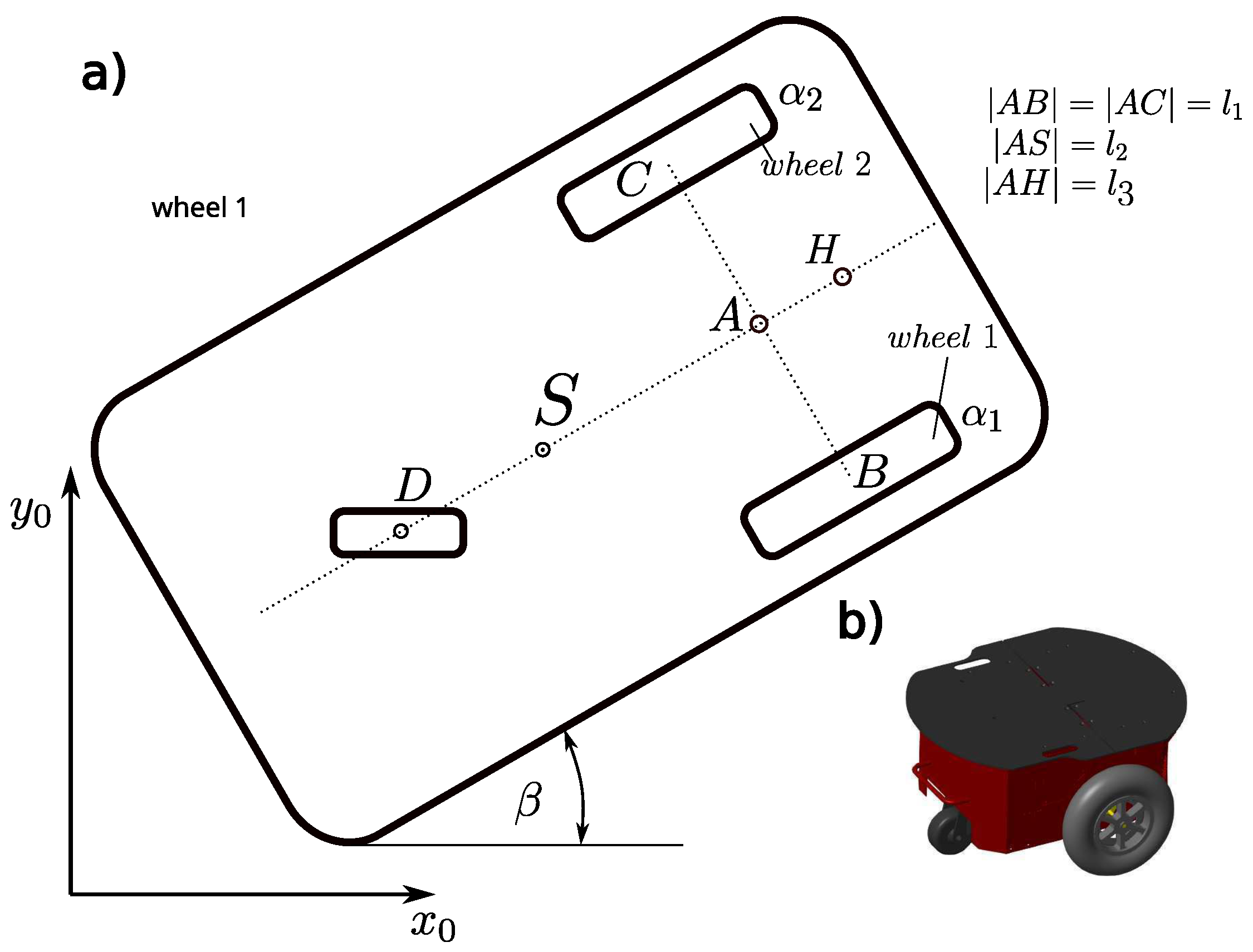
Figure 2.
Scheme of the adaptive control system in the tracking task of a mobile wheeled robot
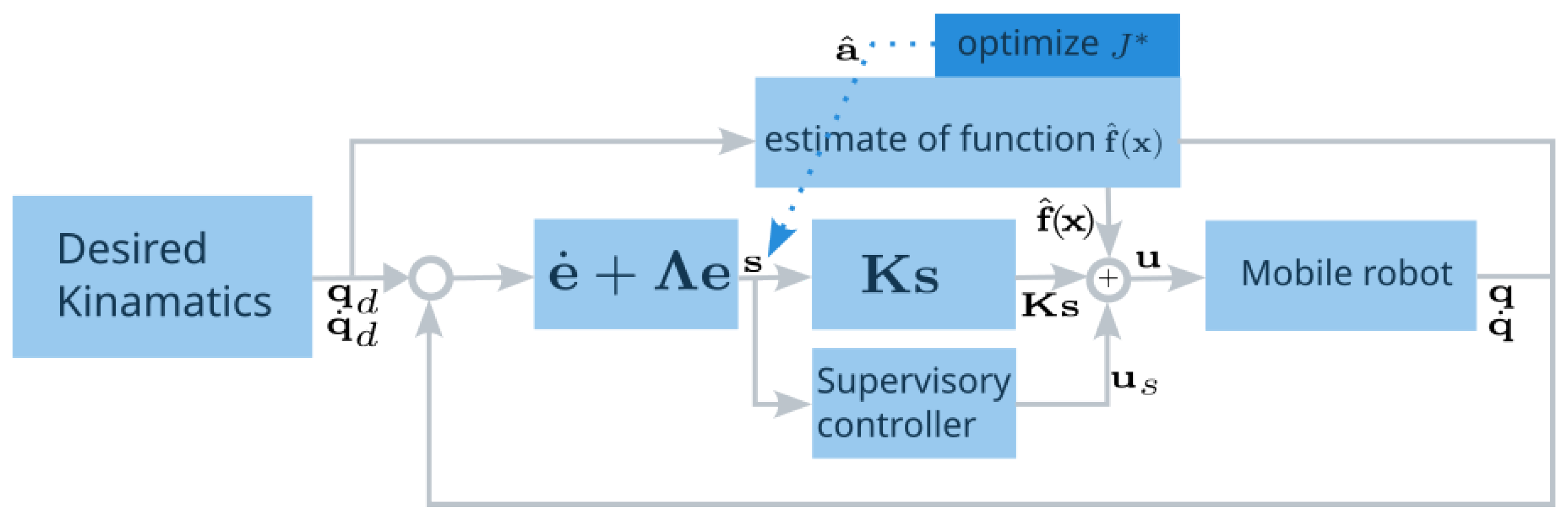
Figure 3.
Values of the coefficient for different values of the parameter
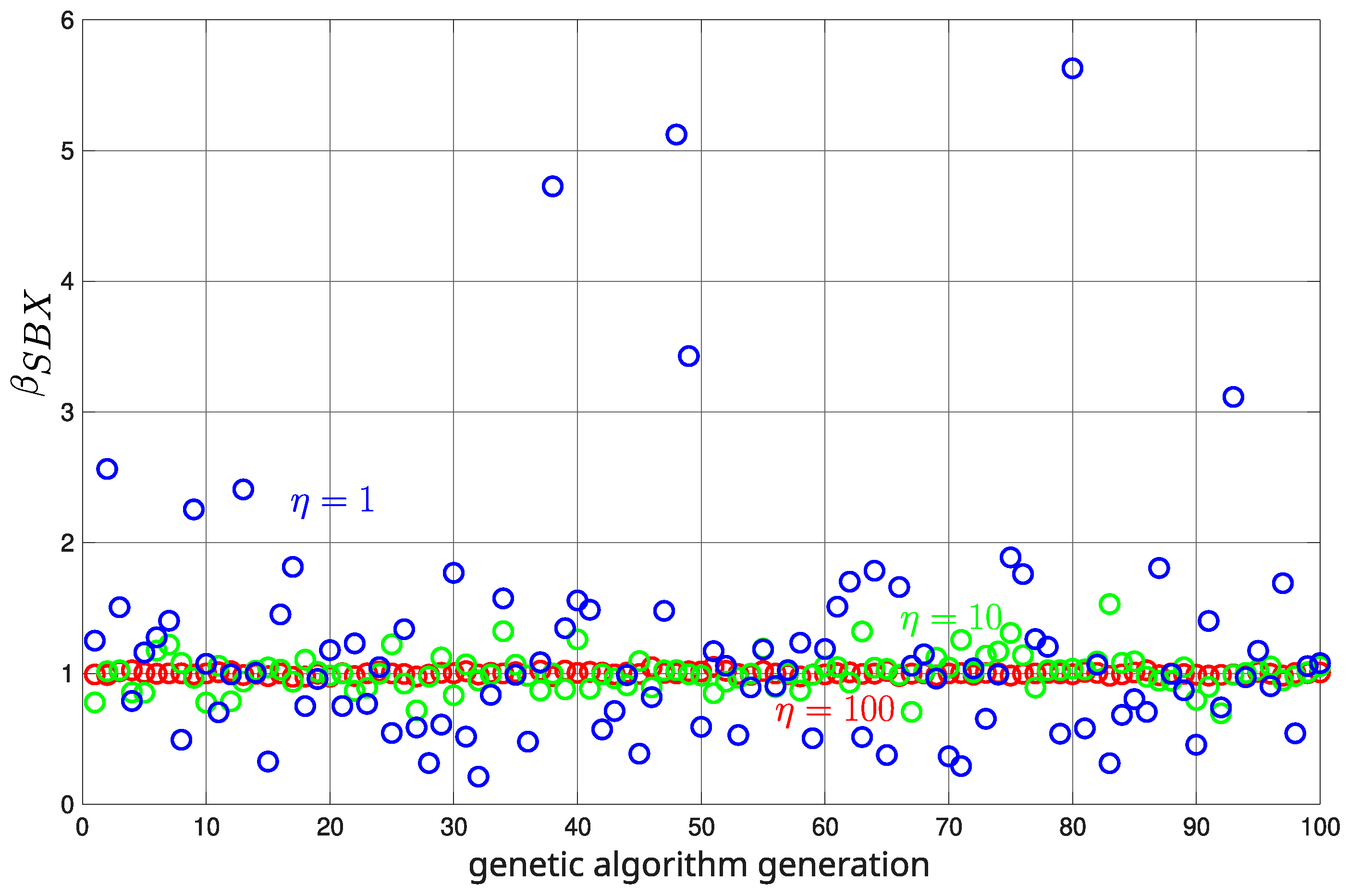
Figure 4.
Przebieg prędkości kół napędzających robota (a) oraz tor ruchu robota kołowego w układzie odniesienia (b)
Figure 4.
Przebieg prędkości kół napędzających robota (a) oraz tor ruchu robota kołowego w układzie odniesienia (b)
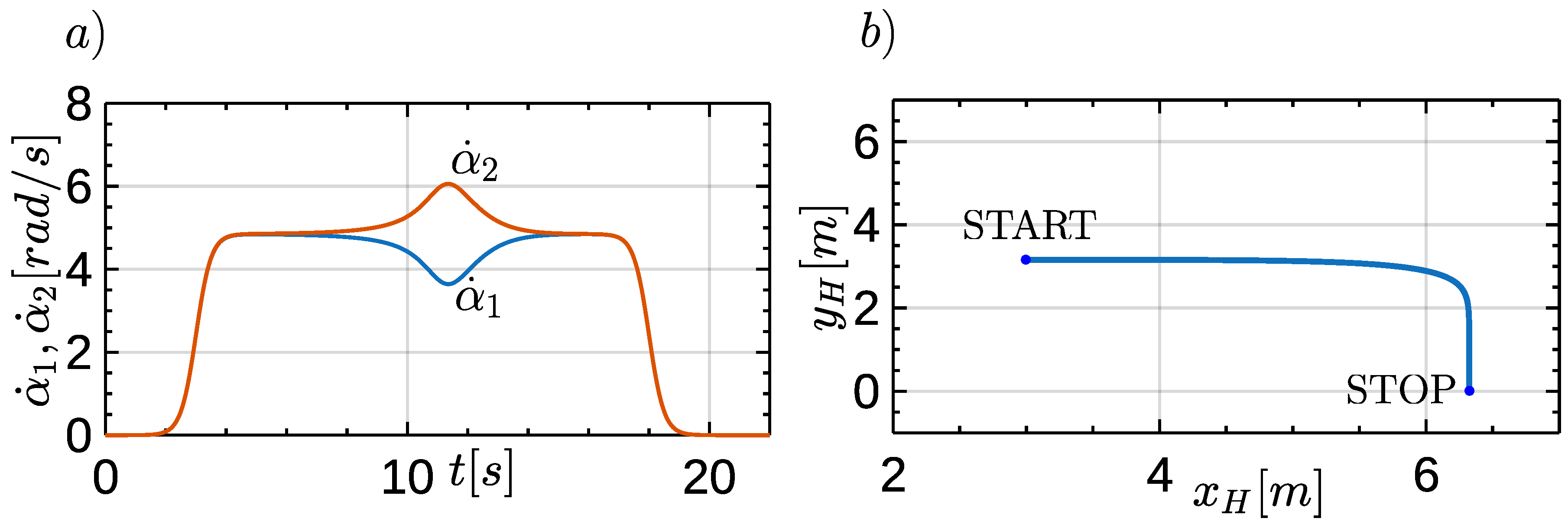
Figure 5.
Control signals: (a) overall control, (b) PD control, (c) compensating controls, (d) filtered tracking error.
Figure 5.
Control signals: (a) overall control, (b) PD control, (c) compensating controls, (d) filtered tracking error.
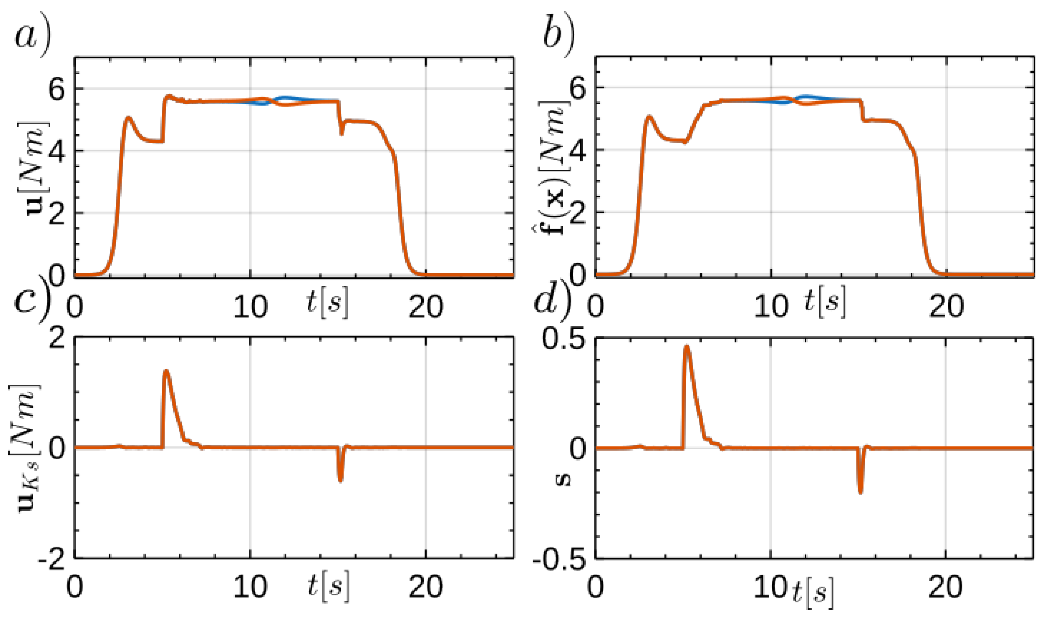
Figure 6.
Course of adaptation of parameter estimates (a) and the fitness function (b).
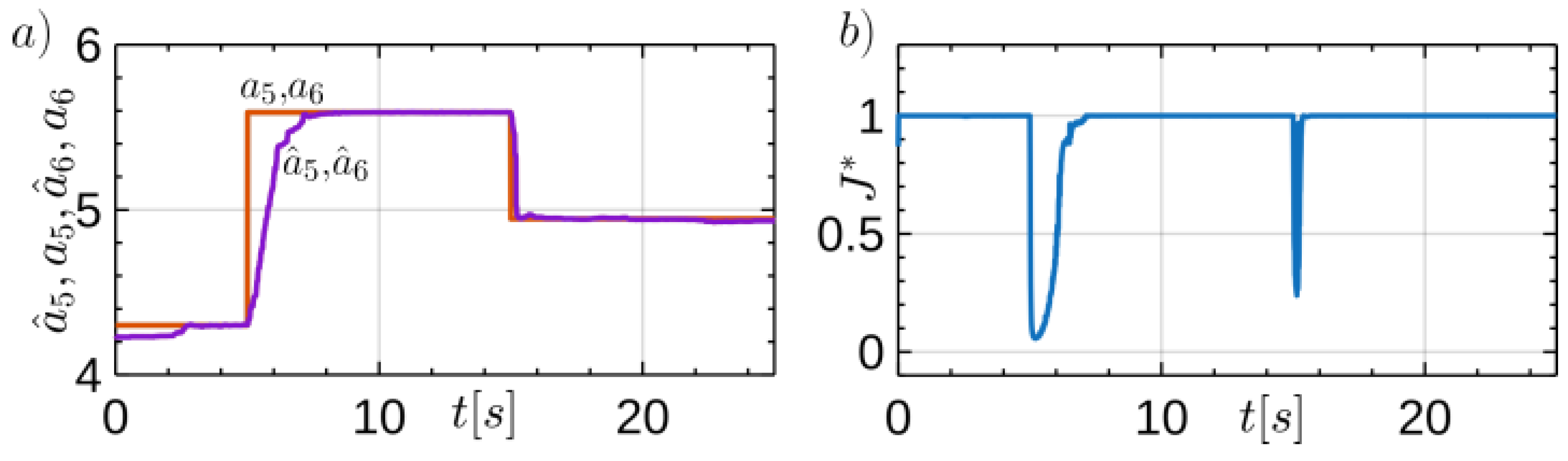
Figure 7.
Tracking error (error waveforms for both wheels have similar values) (a) and desired and obtained angular velocities (b).
Figure 7.
Tracking error (error waveforms for both wheels have similar values) (a) and desired and obtained angular velocities (b).
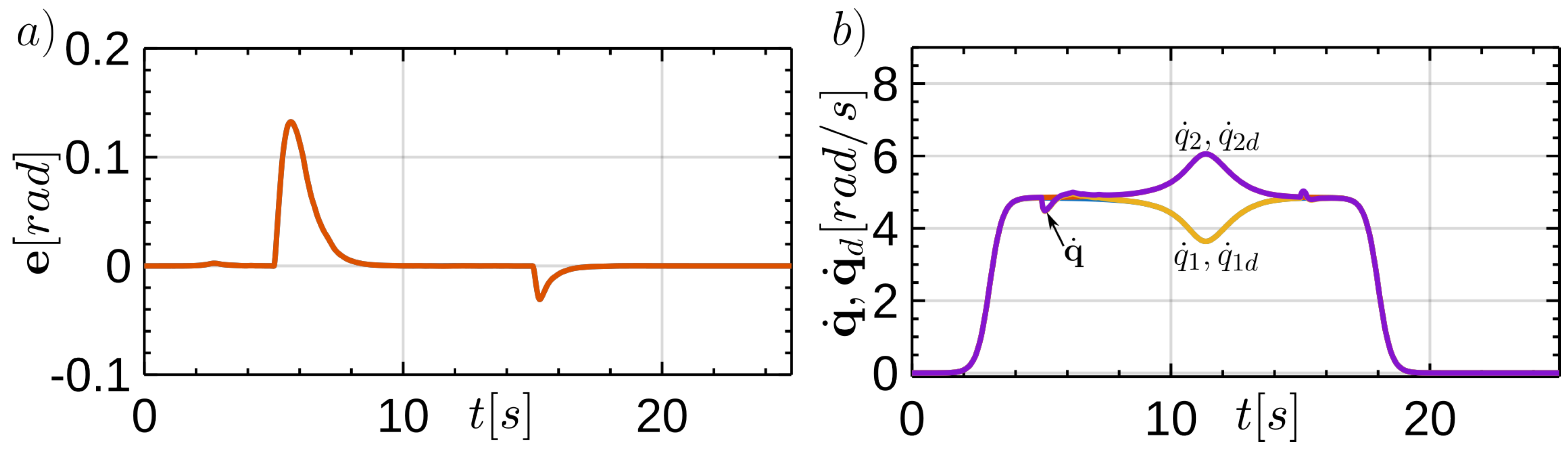

Table 1.
Parameters of the GABONST algorithm in the numerical test.
| Algorithm step according to GABONST procedure | Number of assumption in section 4.5 | Parameters | Determining parameters method based on knowledge |
| (3): condition for the execution of natural selection | 2,3 | ||
| (a): mutation when | 4 | ||
| (i): crossover in natural selection | 5 | ||
| (A): mutation in natural selection | 6 |
Disclaimer/Publisher’s Note: The statements, opinions and data contained in all publications are solely those of the individual author(s) and contributor(s) and not of MDPI and/or the editor(s). MDPI and/or the editor(s) disclaim responsibility for any injury to people or property resulting from any ideas, methods, instructions or products referred to in the content. |
© 2025 by the authors. Licensee MDPI, Basel, Switzerland. This article is an open access article distributed under the terms and conditions of the Creative Commons Attribution (CC BY) license (http://creativecommons.org/licenses/by/4.0/).
Copyright: This open access article is published under a Creative Commons CC BY 4.0 license, which permit the free download, distribution, and reuse, provided that the author and preprint are cited in any reuse.


