Submitted:
12 April 2025
Posted:
30 April 2025
You are already at the latest version
Abstract
Physics-Informed Neural Networks (PINNs) represent a rapidly evolving class of scientific machine learning models that tightly integrate physical laws, typically expressed as partial differential equations (PDEs), into neural network training. By embedding differential constraints directly into the loss function, PINNs enable data-efficient, mesh-free, and equation-consistent approximations of complex physical systems. Over the past few years, PINNs have emerged as a compelling framework for a wide range of forward and inverse problems across disciplines such as fluid dynamics, material science, electromagnetism, biomechanics, and geophysics. This survey provides a comprehensive and critical review of the current state of PINNs. We begin by establishing the mathematical foundations and core architecture of PINNs, illustrating how governing equations, boundary conditions, and measurement data can be unified within a single learning framework. We then explore recent architectural advances and algorithmic innovations, including domain decomposition (e.g., XPINNs), adaptive sampling, spectral PINNs, and stochastic extensions, that address challenges related to scalability, convergence, and uncertainty quantification. Furthermore, we examine benchmark problems, evaluation protocols, and application-specific customizations that have shaped the empirical development of the field. The survey also delves deeply into the limitations of existing approaches, including optimization difficulties, issues in capturing multi-scale and discontinuous phenomena, generalization gaps, and interpretability concerns. We articulate open research challenges and outline emerging directions such as operator learning, meta-learning, hybrid neural-simulation frameworks, neurosymbolic PINNs, and hardware-efficient implementations. By unifying theory, practice, and future vision, this survey aims to serve as a foundational reference for researchers and practitioners across scientific computing, applied mathematics, and machine learning. As PINNs continue to evolve, they offer the promise of enabling a new paradigm of physics-aware, data-driven modeling that is both computationally efficient and scientifically grounded.
Keywords:
Physics-Informed Neural Networks (PINNs)
; Scientific Machine Learning
; Partial Differential Equations
; Neural Operators
; Physics-based Deep Learning
; Surrogate Modeling
; Inverse Problems
; Uncertainty Quantification
; Data-Driven Modeling
; Computational Physics
1. Introduction
The fusion of data-driven learning paradigms with the fundamental laws of physics has emerged as a transformative approach in scientific machine learning (SciML) [1]. Among the most prominent and rapidly advancing frameworks in this domain are Physics-Informed Neural Networks (PINNs), a class of neural network models designed to integrate physical laws, typically represented as partial differential equations (PDEs), directly into the training process. Introduced by Raissi et al [2]. (2019), PINNs have since witnessed an exponential growth in both academic research and practical applications, fueled by the urgent need for interpretable, generalizable, and data-efficient machine learning models in science and engineering [3]. Traditional neural networks excel at function approximation and pattern recognition tasks, but often struggle when applied to domains characterized by scarce or noisy data, or where the governing dynamics are well understood but difficult to solve analytically. PINNs address this gap by embedding the residuals of differential equations into the loss function of a neural network [4]. This enables the network to not only fit available observational data but also to adhere to the physical laws underlying the data. As such, PINNs provide a compelling solution to inverse problems, surrogate modeling, and forward simulations across a wide array of disciplines including fluid mechanics, structural engineering, quantum mechanics, and biomedical imaging [5]. The rise of PINNs can be contextualized within the broader movement towards physics-based learning, where the goal is to synergistically leverage prior scientific knowledge and data [6]. This hybrid modeling philosophy contrasts with the purely data-driven approaches that dominate contemporary deep learning and has profound implications for the generalizability, interpretability, and sample efficiency of neural models [7]. By enforcing physical constraints during training, PINNs can extrapolate more reliably beyond observed data, inherently obey conservation laws, and exhibit greater robustness to noise—properties that are indispensable in mission-critical scientific and engineering applications [8]. PINNs represent a confluence of ideas from computational physics, numerical analysis, and machine learning [9]. They draw upon automatic differentiation for computing derivatives efficiently, variational formulations of PDEs for constructing loss functions, and advanced training strategies to navigate the often stiff optimization landscape that arises from the multi-objective nature of enforcing both data fidelity and physical consistency. Recent advances in PINNs have extended the framework to accommodate complex boundary conditions, multi-physics couplings, stochastic differential equations, and high-dimensional systems, thus significantly broadening their scope and capability [10]. However, despite their promise, PINNs are not without challenges. The training of PINNs can be notoriously difficult due to issues such as gradient imbalance, stiffness in the optimization landscape, and sensitivity to hyperparameters. Moreover, the naive inclusion of physical constraints in the loss function can lead to slow convergence or suboptimal solutions, especially in the presence of complex or multi-scale dynamics. These limitations have spurred a rich body of research aimed at improving the theoretical understanding, architectural design, and training methodologies of PINNs [11]. This survey aims to provide a comprehensive and critical overview of the field of Physics-Informed Neural Networks. We begin by formalizing the PINN framework and its mathematical foundations, including the treatment of different types of differential equations (e.g., elliptic, parabolic, hyperbolic), initial and boundary conditions, and variational principles [12]. We then delve into the diverse landscape of PINN architectures and training techniques, highlighting innovations such as adaptive loss weighting, curriculum learning, domain decomposition, and transfer learning [13]. We also discuss the theoretical underpinnings of PINNs, including convergence guarantees, expressivity, and error bounds, and compare them to classical numerical solvers and other hybrid modeling paradigms. In the latter part of the survey, we review the extensive applications of PINNs across various scientific domains, categorizing them by problem type and assessing their empirical performance [14]. We also examine several extensions and generalizations of PINNs, including stochastic PINNs, operator learning approaches, and methods incorporating uncertainty quantification [15]. Finally, we identify open research challenges and future directions, including the integration of PINNs with symbolic regression, multi-fidelity learning, and reinforcement learning, as well as their deployment in real-time and large-scale computational environments. In summary, Physics-Informed Neural Networks represent a significant stride towards the integration of machine learning with the established principles of scientific modeling [16]. Their ability to embed physical laws into learning algorithms holds the potential to revolutionize scientific computing, enabling more accurate, efficient, and interpretable models [17]. Through this survey, we aim to consolidate the current state of the art, foster a deeper understanding of the underlying principles, and inspire future research at the intersection of physics, machine learning, and numerical computation.
2. Mathematical Formulation and Framework
Physics-Informed Neural Networks (PINNs) are designed to solve supervised learning tasks while simultaneously enforcing physical laws expressed by partial differential equations (PDEs). This section formalizes the general PINN framework using rigorous mathematical notation and graphical representation.
2.1. Problem Setting
Let be a spatial domain with boundary , and let be a time domain [18]. The goal is to approximate the solution of a general PDE of the form:
subject to initial and boundary conditions:
2.2. Loss Function Construction
The neural network is trained by minimizing a composite loss function:
where each component is defined as:
Here, , , and represent collocation points in the interior, initial, and boundary domains, respectively [20]. The hyperparameters control the relative importance of each term.
2.3. Architectural Variants
The table below summarizes several prominent variants of PINNs that address different challenges such as stiffness, multi-scale features, and uncertainty quantification.

Table 1.
Comparison of Common PINN Variants.
| Method | Core Idea | Target Problem | Reference |
|---|---|---|---|
| Vanilla PINN | PDE residual in loss | General PDEs | Raissi et al. (2019) |
| XPINN | Domain decomposition | Multi-scale domains | Jagtap et al [21]. (2020) |
| fPINN | Fourier features | High-frequency solutions | Wang et al. (2021) |
| UQ-PINN | Probabilistic weights | Uncertainty quantification | Yang et al. (2021) |
| hp-PINN | Adaptive meshing and depth | Stiff problems | Lu et al. (2022) |
2.4. Neural Network Architecture
3. Training Strategies and Optimization Techniques
Despite their conceptual elegance and theoretical appeal, training Physics-Informed Neural Networks (PINNs) presents significant practical challenges [23]. The interplay between data-driven loss and physical residuals often results in a multi-objective optimization landscape that is stiff and highly sensitive to hyperparameters. This section discusses the common issues that arise during training and the state-of-the-art strategies proposed to overcome them.
3.1. Optimization Challenges
The total loss in PINNs consists of terms of potentially different scales and numerical stiffness [24]:
This formulation introduces a trade-off between learning from data and satisfying the PDE constraints [25]. In practice, can dominate or vanish compared to boundary and initial losses, leading to poor generalization or trivial solutions [26]. Additionally, the gradients of higher-order derivatives in the PDE residual can cause vanishing or exploding gradients, impeding convergence.
3.2. Gradient Pathologies and Stiffness
Recent work by Wang et al. (2021) and Krishnapriyan et al. (2021) showed that PINNs suffer from pathological gradient flows. The dominant eigenvalues of the PDE Jacobian may lead to ineffective updates, a phenomenon termed "gradient pathologies." These issues become more pronounced in multi-scale PDEs or problems with steep gradients and sharp interfaces.
3.3. Training Enhancements
3.4. Optimization Algorithms
PINNs are typically trained using first-order optimizers such as Adam, often followed by second-order optimizers like L-BFGS to refine convergence. The combined strategy is formalized as [31]:
This two-stage approach exploits the fast convergence of L-BFGS while benefiting from Adam’s stochasticity to escape local minima early in training.
3.5. Training Pipeline Overview
The schematic in Figure 2 outlines the high-level training loop of a typical PINN, including forward pass, automatic differentiation, loss evaluation, and optimization.
4. Theoretical Foundations and Analysis
While Physics-Informed Neural Networks (PINNs) have demonstrated impressive empirical success, understanding their theoretical properties is essential for establishing their reliability, robustness, and scope of applicability. This section presents a comprehensive overview of the foundational principles that underpin the behavior of PINNs, including their approximation capabilities, convergence characteristics, generalization bounds, and fundamental limitations [32]. We also highlight recent results that connect PINNs to classical numerical schemes and propose open problems in formalizing their behavior.
4.1. Universal Approximation and PDE Solutions
At the core of the PINN framework lies the universal approximation theorem, which guarantees that neural networks with sufficient width and depth can approximate any continuous function on a compact set, given appropriate activation functions. In the context of PDEs, this implies that there exists a neural network such that:
for any , where denotes the true solution to the PDE [33]. However, approximation alone does not ensure convergence of the training process. In practice, neural networks may fail to recover unless the loss landscape facilitates effective optimization and the PDE constraints are adequately enforced [34]. Recent theoretical studies have analyzed the representational capacity of PINNs in the context of Sobolev spaces [35]. For example, Lu et al [36]. (2021) showed that for certain classes of elliptic and parabolic PDEs, neural networks can approximate the solution with bounded error in the or norm [37]. These results provide a bridge between the classical theory of weak solutions and modern deep learning approximators.
4.2. Error Decomposition and Convergence Guarantees
The total error in a PINN approximation can be decomposed into three components:
- Approximation error: Due to the finite capacity of the neural network.
- Optimization error: Due to incomplete minimization of the loss function.
- Generalization error: Due to the finite number of training points.
Formally, for a loss functional and empirical risk over a sample set , we can write [38]:
The optimization error is often exacerbated by the stiffness of the PDE and the imbalance between loss components. Adaptive optimization methods, while empirically helpful, lack convergence guarantees in non-convex, multi-objective settings like PINNs [39]. Recent works, such as those by Mishra and Molinaro (2022), have started to establish convergence rates under specific conditions, such as linear PDEs with well-behaved residuals [40].
4.3. Generalization in Function Space
Unlike classical supervised learning, where generalization refers to performance on unseen data, PINNs must generalize over a continuous function space defined by the PDE’s solution manifold. This raises the question: How well can a neural network trained on a finite set of collocation points generalize to the infinite-dimensional solution space? Babuska et al. (2021) analyzed this problem using statistical learning theory in Sobolev spaces. They established upper bounds on the generalization error of PINNs under certain assumptions on the smoothness of the solution and the distribution of training points [41]. Their findings suggest that dense and adaptively chosen collocation points can significantly improve generalization, especially in regions with high residual variance. Another promising line of work views PINNs through the lens of operator learning. In this perspective, the network learns not just a function, but an operator mapping from the coefficients of the PDE to its solution. This interpretation aligns with recent developments in DeepONets and Fourier Neural Operators (FNOs), which provide theoretical insights into learning solution operators in Banach spaces [42].
4.4. Comparison with Classical Numerical Methods
A key theoretical question is whether PINNs can match or surpass the performance of traditional numerical solvers such as finite difference, finite volume, or finite element methods. While PINNs offer mesh-free solutions and can handle irregular geometries and sparse data, their convergence rates are not yet as well-characterized as those of classical solvers [43]. The work of Karniadakis et al. (2021) draws a connection between PINNs and Galerkin methods, showing that under certain conditions, the PINN loss function can be interpreted as a variational residual, similar to a weak form in the finite element method. This equivalence provides a foundation for hybrid schemes that combine the best of both worlds: the flexibility of neural networks and the precision of numerical discretization.
4.5. Limitations and Open Problems
Despite the progress, several theoretical challenges remain open:
- There is no universal guidance for choosing the collocation point distribution, network architecture, or loss weights that guarantee convergence for arbitrary PDEs [44].
- PINNs often struggle with sharp discontinuities and multi-scale features, where classical solvers are more robust due to explicit mesh refinement and adaptivity [45].
- The impact of network depth and width on approximation accuracy in the presence of stiff differential operators is not fully understood.
- It remains an open question how to formally characterize the solution manifold of complex PDE systems and how this geometry interacts with the inductive bias of neural networks.
In summary, while PINNs inherit the expressive power of deep neural networks and introduce physics-based constraints to improve generalization, their theoretical understanding is still in its early stages [46]. Ongoing work in approximation theory, optimization landscapes, and statistical learning is essential to transform PINNs from empirical tools into rigorously grounded methods for scientific computation [47].
5. Applications Across Scientific and Engineering Domains
The integration of deep learning with domain-specific physical laws has enabled Physics-Informed Neural Networks (PINNs) to penetrate a wide array of scientific and engineering disciplines. The data-efficiency, mesh-free nature, and capacity to enforce governing equations without discretization have made PINNs an attractive alternative to traditional solvers in scenarios where data is sparse, boundary conditions are complex, or computational cost is prohibitive [48]. This section surveys notable application areas where PINNs have demonstrated practical utility, highlighting representative case studies, model configurations, and domain-specific adaptations [49].
5.1. Fluid Mechanics and Navier–Stokes Solvers
One of the earliest and most impactful domains where PINNs have shown promise is computational fluid dynamics (CFD) [50]. The Navier–Stokes equations, which govern fluid motion, are notoriously difficult to solve due to their nonlinearity and the presence of multiscale structures, turbulence, and complex boundaries [51]. Raissi et al. (2019) applied PINNs to infer velocity and pressure fields from limited flow data, successfully recovering full flow fields in canonical problems such as the lid-driven cavity and flow around a cylinder [52]. Incompressible Navier–Stokes equations take the form:
where is the velocity field, p is pressure, and is kinematic viscosity [53]. PINNs approximate both and p using neural networks while ensuring that the PDE and continuity equation are satisfied at collocation points. Subsequent research has extended these ideas to turbulent flows using multi-network architectures, temporal decomposition, and data assimilation techniques. Chen et al [54]. (2021) introduced a turbulence-aware PINN framework that blends sparse experimental data with Reynolds-averaged Navier–Stokes (RANS) equations for closure modeling [55].
5.2. Solid Mechanics and Material Modeling
PINNs have also found significant use in elasticity and plasticity simulations, especially in problems involving complex geometries or material heterogeneity. The governing PDEs in linear elasticity, such as:
are well-suited for the PINN framework, with stress–strain relationships embedded directly into the loss formulation [56]. Haghighat et al [57]. (2020) applied PINNs to simulate stress fields in heterogeneous media, such as composites and anisotropic materials. PINNs were also used to discover material constitutive laws directly from displacement or strain data, opening up new possibilities for inverse problems in solid mechanics. Recent hybrid approaches combine PINNs with finite element methods (FEM), yielding hybrid-FEM PINNs that improve accuracy near boundaries while reducing computational overhead in bulk regions [58].
5.3. Electromagnetics and Wave Propagation
In electromagnetics, PINNs have been applied to Maxwell’s equations, wave propagation, and photonic design problems. These applications are particularly well suited to PINNs due to the high dimensionality and difficulty of mesh generation in complex dielectric geometries [59]. For instance, the time-domain Maxwell’s equations:
have been modeled using PINNs to simulate electric and magnetic fields in media with spatially varying permittivity and permeability. Tezuka et al [60]. (2021) used PINNs to design metasurfaces and photonic crystals by solving the inverse scattering problem using electromagnetic PDE constraints. Moreover, the Schrödinger equation, central to quantum wave propagation, has been addressed with PINNs for applications in quantum control and nanophotonics, demonstrating accurate wavefunction inference from sparse measurement data.
5.4. Biomedical Applications and Physiology Modeling
The biomedical field offers numerous challenges involving partial differential equations with irregular domains, noisy measurements, and patient-specific geometries. PINNs have emerged as a promising tool to model blood flow, electrophysiology, and tissue mechanics from clinical imaging and sensor data. Kissas et al. (2020) applied PINNs to cardiovascular flows by solving the Navier–Stokes equations in three-dimensional patient-specific aortic geometries reconstructed from MRI data [61]. Their approach enabled real-time inference of pressure and velocity fields, offering a potential path toward non-invasive diagnostics [62]. Another area of development is the modeling of electrophysiological dynamics in the heart and brain. By enforcing the monodomain or bidomain models through PINN architectures, researchers have recovered transmembrane potentials and ionic currents from surface recordings such as ECG and EEG, effectively transforming sparse sensor data into spatially resolved field quantities [63].
5.5. Energy Systems and Geophysical Simulations
PINNs have been applied in modeling geothermal energy flows, subsurface transport, and seismic wave propagation—domains where traditional mesh-based methods can be computationally intensive due to large domain sizes and geological complexity [64]. In geothermal systems, PINNs have been used to simulate temperature and pressure fields governed by Darcy’s law and advection-diffusion equations. Shukla et al [29]. (2021) applied PINNs to estimate thermal conductivity and permeability from sparse well data. Seismic inversion is another critical application where PINNs have provided robust results. By solving the elastic wave equation with unknown initial and boundary conditions, PINNs can reconstruct subsurface velocity models from limited seismic signals, offering an alternative to computationally expensive adjoint-based methods [14].
5.6. Summary of Application Landscape
Figure 3 visually summarizes the breadth of domains in which PINNs have been applied, along with the corresponding PDE families and data sources.
6. Hybrid Architectures and Extensions of PINNs
While the original formulation of Physics-Informed Neural Networks (PINNs) demonstrates a novel and flexible framework for solving differential equations using neural approximators, numerous practical limitations have prompted the development of a wide range of extensions and architectural variants. Chief among these limitations are poor scalability to high-dimensional and stiff PDEs, degradation of accuracy in long-time simulations, difficulty in handling discontinuities and multi-scale features, and lack of domain-specific adaptivity [7]. To address these issues, researchers have proposed hybrid architectures, domain-decomposition strategies, and new classes of operator learning models that generalize or complement the classical PINN paradigm [65].
6.1. XPINNs: Domain Decomposition for Parallelization
XPINNs (Extended PINNs), proposed by Jagtap et al [66]. (2020), are designed to overcome one of the most pressing limitations of PINNs: their poor scalability to large domains and multi-physics systems. XPINNs leverage a space-time domain decomposition strategy in which separate neural networks are trained in overlapping or non-overlapping subdomains. Each subdomain imposes continuity conditions at interfaces:
where denotes the interface region and are solutions in adjacent subdomains [67]. XPINNs enable distributed training and support problem-specific adaptivity, making them attractive for high-performance computing applications.
6.2. cPINNs: Conservative PINNs for Physical Consistency
Conservative PINNs (cPINNs), introduced by Mao et al [68]. (2020), are particularly suitable for PDEs that possess strong conservation laws [69]. While standard PINNs minimize residual loss functions, they may violate integral conservation properties. cPINNs incorporate integral form constraints directly into the loss:
thereby ensuring that global physical laws—such as mass, momentum, or energy conservation—are honored throughout the domain [70]. These formulations have shown improved stability in applications such as shallow water equations and conservation-driven fluid dynamics.
6.3. hpPINNs: Multi-Resolution Refinement Strategies
Multi-scale PDEs—such as those in turbulent flows, porous media, or chemical kinetics—often contain fine-scale structures that cannot be captured effectively with standard PINNs. hpPINNs (hierarchical + partitioned PINNs) address this by drawing inspiration from -adaptive finite element methods [71]. The domain is divided into multiple subregions, each associated with a different network that may vary in depth (h-adaptivity) and width (p-adaptivity). This approach allows for dynamic refinement in regions with high PDE residuals, using an indicator function:
where is the differential operator. Subdomains with above a threshold are split recursively and assigned higher-capacity networks. This method enables the construction of surrogate solutions with high local accuracy and global efficiency.
6.4. DeepONets and Neural Operators
While PINNs focus on learning solutions for a fixed PDE, a growing body of work aims to learn the operator that maps inputs (e.g., coefficients, boundary conditions, source terms) to the solution function:
where f may represent initial conditions or PDE parameters. DeepONets (Lu et al., 2021) are among the earliest operator learning frameworks, designed to approximate nonlinear operators through a two-branch network:
- The branch net encodes the input function f sampled at sensors .
- The trunk net encodes the target location x.
- The output is .
Another prominent class of models is the Fourier Neural Operator (FNO), which performs convolution in the Fourier domain to learn global interactions. These models have demonstrated state-of-the-art performance in learning solution operators of parametric PDEs like the Darcy flow equation and Navier–Stokes dynamics at high resolution, significantly reducing inference cost.
6.5. Variational, Probabilistic, and Multi-Modal Extensions
Beyond deterministic solvers, several extensions aim to incorporate uncertainty quantification, stochasticity, and variational principles:
- Bayesian PINNs use variational inference or Hamiltonian Monte Carlo to estimate posterior distributions over the solution u or parameters , enabling uncertainty-aware predictions [72].
- Variational PINNs (VPINNs) reformulate the training objective as a variational minimization, inspired by finite element weak formulations:where are test functions in a Hilbert space.
- Multi-modal PINNs integrate diverse data modalities—such as pointwise measurements, images, and boundary sensor arrays—by encoding each modality into a shared latent space before applying PDE constraints. This is particularly powerful in biomedical imaging and remote sensing.
6.6. Summary and Design Taxonomy
Table 3 summarizes key PINN extensions along with their core objectives and distinguishing features.
These innovations collectively expand the reach of physics-informed learning beyond the classical PINN framework. They address critical bottlenecks in efficiency, accuracy, and flexibility, enabling more robust and scalable neural PDE solvers for real-world scientific computing.
7. Evaluation, Benchmarks, and Performance Metrics
As the field of physics-informed learning matures, the demand for rigorous, standardized evaluation of PINN-based models has become increasingly pronounced. Unlike conventional machine learning tasks that enjoy well-established benchmarks and metrics (e.g., ImageNet, GLUE), physics-informed neural networks operate across a diverse array of PDEs, geometries, and scientific domains—making evaluation particularly challenging. In this section, we provide a structured review of current practices for benchmarking PINNs, focusing on error metrics, test scenarios, computational performance, and reproducibility considerations.
7.1. Quantitative Metrics for PINN Evaluation
Evaluation metrics for PINNs are inherently tied to the continuous nature of the underlying PDE solutions. Below, we list the most common quantitative metrics used across studies:
- Relative Error:where is the predicted solution and is the ground truth from analytical or high-fidelity numerical solvers.
- Pointwise Residual Error: Measures how well the predicted solution satisfies the governing PDE:where are collocation points and is the PDE operator.
- Boundary Error: Quantifies the deviation at boundaries:where g is the specified boundary condition [73].
- Conservation Loss: For problems with integral conservation laws (e.g., mass, energy), the global integral of the discrepancy is evaluated.
- Computation Time and Scalability: Total training time, GPU/CPU utilization, and memory footprint are critical performance measures, particularly for large-scale applications [74].
In practice, studies often report a mix of these metrics across multiple test scenarios, highlighting trade-offs between physical fidelity, numerical accuracy, and efficiency.
7.2. Common Benchmark Problems and Datasets
Several canonical PDEs and synthetic datasets have emerged as de facto benchmarks in the PINN literature [75]. These allow for direct comparison of model performance and facilitate reproducibility. Table 4 summarizes commonly used benchmark problems across different domains [76].
In addition to synthetic PDE problems, a growing number of datasets incorporate experimental data, such as Particle Image Velocimetry (PIV) flows, physiological recordings (e.g., MRI, ECG), and geophysical sensor data [77].
7.3. Ablation Studies and Model Diagnostics
Modern PINN studies increasingly include ablation experiments to isolate the effects of architectural components, training schedules, and loss weighting schemes [38]. Representative diagnostic axes include:
- Activation Function Sensitivity: Comparing tanh, ReLU, GELU, sine activations for convergence behavior.
- Network Depth and Width: Impacts expressivity vs. trainability trade-offs.
- Gradient Pathologies: Monitoring gradient norms and Hessian spectra to detect vanishing/exploding gradients or stiffness [78].
- Loss Weighting Strategies: Empirical comparisons between fixed, dynamic, and adaptive loss weighting.
Such diagnostics are increasingly supported by automated PINN frameworks such as DeepXDE, NeuralPDE, and SimNet.
7.4. Reproducibility and Open-Source Benchmarks
The reproducibility of PINN-based research is still an ongoing concern due to the complex interaction between data, physics constraints, and optimization [79]. Fortunately, several open-source libraries and community benchmarks have emerged:
- DeepXDE (Lu et al.): TensorFlow-based library for solving differential equations with PINNs and DeepONets.
- NeuralPDE.jl (SciML): A Julia-based framework emphasizing scientific machine learning with strong PDE support.
- PINNBench: A curated benchmark suite with standardized problem definitions, metrics, and logging.
- NSFnets, PhyCRNet: PyTorch-based specialized PINN variants for fluid dynamics and conservation laws.
7.5. Challenges in Evaluation and Future Needs
Despite progress, several challenges persist in benchmarking PINNs:
- Lack of Standard Baselines: Results across papers are often not directly comparable due to differing training protocols, data sampling schemes, and evaluation regions.
- Inconsistent Reporting: Studies may report only error metrics, omitting critical training diagnostics such as convergence time or gradient behavior.
- No Ground Truth for Real-World Inverse Problems: In many scientific applications, the exact solution is unknown, making surrogate benchmarking difficult [82].
- Neglected Generalization Metrics: PINNs are rarely evaluated on their ability to generalize across PDE parameters, geometries, or domains—an important aspect for true operator learning.
There is a growing push toward community-defined evaluation protocols, complete with challenge datasets, cross-lab comparisons, and formal reproducibility checklists—akin to initiatives in NLP and computer vision. Such efforts will be instrumental in benchmarking PINNs rigorously and ensuring robust scientific contributions.
8. Challenges, Limitations, and Open Problems
Despite the remarkable promise and growing adoption of Physics-Informed Neural Networks (PINNs), the field faces several formidable challenges that hinder its widespread applicability in scientific and engineering workflows. These challenges span across optimization theory, numerical analysis, generalization behavior, and system integration [75]. In this section, we offer a comprehensive critique of the known limitations of PINNs and identify open research questions that require resolution for the field to mature.
8.1. Optimization Landscape and Training Instabilities
One of the most persistent challenges in training PINNs is the difficulty of optimizing the composite loss function, which blends data fitting with differential equation residuals. This typically leads to ill-conditioned and non-convex loss surfaces. Empirical studies have demonstrated that:
- The PDE residual component of the loss may exhibit high stiffness, leading to vanishing gradients in early layers (gradient pathologies).
- The loss terms may have significantly different magnitudes, necessitating sophisticated loss balancing or dynamic reweighting schemes (e.g., NTK-based weights, adaptive residual weighting).
- Overparameterized networks often converge to poor minima that satisfy the data terms but poorly approximate the solution manifold.
Recent works have attempted to address these issues via curriculum learning, residual-based adaptive sampling, Sobolev training, and second-order optimizers, yet no universally robust method exists. Theoretical understanding of the optimization dynamics in PINNs remains limited, especially in high dimensions.
8.2. Expressivity and Approximation Theory
While universal approximation theorems guarantee that neural networks can represent PDE solutions under ideal conditions, the ability of PINNs to approximate complex, multi-scale, or discontinuous solutions remains in question [83]. In particular:
- PINNs struggle to capture sharp gradients, shocks, or discontinuities, such as those found in hyperbolic PDEs and multiphase flows.
- In multi-scale problems (e.g., turbulent flow), the global nature of the neural representation may smooth out fine-grained features unless explicitly encoded using hierarchical or Fourier-based structures.
- There is a lack of a priori error bounds or convergence guarantees for PINNs under general conditions.
Efforts such as hpPINNs, wavelet neural operators, and local basis PINNs have shown promise, but the formal approximation theory for PINNs—particularly in the presence of PDE singularities—remains an open research frontier [84].
8.3. Scalability and High-Dimensional PDEs
The scalability of PINNs to high-dimensional and long-time simulation problems is another major bottleneck [85]. While traditional mesh-based solvers suffer from the curse of dimensionality due to exponential growth in grid points, PINNs are expected to offer mesh-free alternatives. However, in practice:
- The number of collocation points and gradient evaluations increases steeply with the problem size.
- Training time grows nonlinearly with input dimension, limiting use in climate models, molecular dynamics, or plasma physics where .
Emerging solutions include dimensionality reduction via autoencoders, latent PINNs, domain decomposition (XPINNs), and distributed training. However, truly scalable PINN solvers for high-dimensional PDEs remain elusive.
8.4. Data-Physics Conflicts and Label Inconsistency
In real-world settings, observational data may be noisy, sparse, or inconsistent with the governing equations [87]. PINNs are often tasked with simultaneously fitting data and satisfying PDE constraints, which leads to a trade-off known as the data-physics conflict. This conflict manifests in:
- Overfitting to noisy or incorrect labels at the expense of physical fidelity.
- Inability to resolve model discrepancies due to unmodeled physics, missing terms, or coarse discretization.
- Instability in inverse problems where the ground truth is ill-posed or ambiguous.
Probabilistic PINNs, adversarial training, and robust loss functions (e.g., Huber loss) have been proposed to mitigate this issue, but there is still a lack of principled frameworks for uncertainty-aware, conflict-resolving PINN training [88].
8.5. Generalization and Transfer Learning in PDE Settings
Unlike standard machine learning tasks, where generalization is evaluated over data distributions, generalization in PINNs is far more nuanced [89]. Critical open questions include:
- How do PINNs generalize to new geometries, boundary conditions, or PDE coefficients not seen during training?
- Can pretrained PINNs on a family of PDEs be fine-tuned efficiently (e.g., transfer learning) [31]?
- How robust are PINNs to small perturbations in input conditions or model parameters?
Recent advances in operator learning (e.g., DeepONets, FNOs) offer partial answers by explicitly learning mappings between function spaces, but robust generalization across PDE families remains a largely unsolved problem.
8.6. Interpretability and Physical Insight
Although PINNs are rooted in physics, their internal representations are still black-box neural networks with limited interpretability [90]. This poses a barrier for domain experts who seek to extract scientific insights, identify causal mechanisms, or debug model failures. Key concerns include:
Interpretable PINNs, sparsity-promoting architectures, symbolic regression hybrids, and physics-guided attention mechanisms are promising directions, but are still in their infancy.
8.7. Integration into Scientific Workflows
Finally, the integration of PINNs into end-to-end scientific pipelines remains an open challenge. In practice, deploying PINNs requires:
Efforts like SciML, Modulus, and UQ-enhanced frameworks aim to close this gap, but significant engineering and tooling work is still needed to make PINNs plug-and-play for practicing scientists and engineers.
8.8. Summary of Limitations and Research Gaps
To consolidate the above discussion, we summarize the major limitations and research needs of current PINN methodologies in Table 5.
Addressing these challenges requires interdisciplinary advances across numerical analysis, machine learning, applied physics, and software systems. As the field evolves, these limitations serve not as deterrents but as rich research directions for developing the next generation of physics-informed learning systems.
9. Future Directions and Opportunities
The development of Physics-Informed Neural Networks (PINNs) marks a fundamental shift in how machine learning can interact with and leverage scientific knowledge. Despite their challenges, PINNs have established a foundation upon which next-generation scientific computing frameworks can be built. In this section, we articulate a vision for future research by highlighting emerging opportunities and interdisciplinary directions that promise to extend the capabilities, applicability, and theoretical robustness of PINN-based models [18].
9.1. Hybrid Modeling: Bridging Data and Simulation
One promising direction is the construction of hybrid models that combine data-driven learning with traditional simulation techniques [95]. While PINNs offer a fully neural approach, many scientific applications benefit from domain-specific solvers. Hybrid strategies could:
- Embed numerical solvers as differentiable modules within deep architectures (e.g., physics-informed recurrent solvers).
- Use PINNs to correct or augment coarse-grid solvers, serving as learned subgrid models or data-driven closures [96].
- Couple PINNs with classical methods such as finite elements (FEM) or boundary element methods (BEM) in multi-resolution or multi-physics setups [97].
These approaches allow practitioners to retain the guarantees of classical methods while benefiting from the flexibility and expressiveness of neural networks.
9.2. Probabilistic and Bayesian PINNs
Most current PINNs are deterministic, providing point estimates of the solution [98]. However, scientific decision-making often requires calibrated uncertainty estimates [99]. Future work can explore:
- Bayesian formulations of PINNs using stochastic variational inference or Hamiltonian Monte Carlo.
- Deep ensembles or dropout-based Bayesian approximations to capture epistemic uncertainty.
- PINNs as priors in probabilistic graphical models for inverse problems [100].
Such approaches could unlock the potential of PINNs in safety-critical domains, including medicine, aerospace, and climate forecasting [101].
9.3. Operator Learning and Meta-Learning for PINNs
A foundational advance in recent years is the shift from learning solutions to learning operators—that is, mappings from problem setup to solution space [102]. This perspective enables:
- Meta-learning across PDE families, geometries, or boundary conditions, where a PINN model can adapt rapidly to new tasks [103].
- Learning parameterized PDE solvers as reusable surrogates that generalize beyond single simulations.
- Incorporating differentiable optimization or bilevel learning into the PINN framework for PDE-constrained problems.
Operator learning frameworks such as DeepONets, Fourier Neural Operators (FNOs), and Green’s function-based architectures will likely serve as foundational building blocks in this direction.
9.4. Geometry-Aware and Mesh-Compatible Architectures
Scientific domains often feature complex geometries (e.g., aircraft, organs, porous media) where Euclidean coordinates are inadequate [104]. Future advances in geometry-aware PINNs may include:
- Using graph neural networks (GNNs) or mesh-based convolutions to process non-Euclidean domains.
- Incorporating spectral methods or manifold learning to represent irregular geometries.
- Leveraging symmetry and invariance principles (e.g., gauge symmetries, Lie groups) to inform network architecture.
This would allow PINNs to be deployed natively on CAD geometries, anatomical meshes, or finite-volume domains, enhancing applicability in engineering and biomedical contexts [105].
9.5. Neurosymbolic and Interpretable PINNs
A key long-term goal is the ability to extract interpretable, symbolic knowledge from trained PINNs [106]. Bridging symbolic regression, causal discovery, and deep learning, future work may:
- Develop sparse PINN architectures that can recover underlying governing equations (e.g., Sparse Identification of Nonlinear Dynamics—SINDy).
- Combine neural representations with logic rules or physics ontologies for mixed-symbolic reasoning.
- Enable interactive tools for domain experts to query, interpret, and validate PINN behaviors [107].
Such efforts align with broader goals in neurosymbolic AI and human-centric scientific discovery.
9.6. Hardware-Aware and Real-Time PINNs
Deploying PINNs in real-world environments often demands real-time inference and low-latency computation. Future research should consider:
9.7. Standardization and Community Infrastructure
To foster robust progress, the field would benefit from systematic efforts to build shared infrastructure, including:
- Public benchmark suites with reproducible pipelines and baseline models.
- Domain-specific extensions of PINN toolkits (e.g., for electromagnetics, fluid dynamics, or medical physics) [111].
- Common standards for dataset formats, geometry representation, and loss function design.
- Collaborative platforms for crowdsourced model development and cross-lab evaluations [112].
Lessons from the evolution of NLP and vision suggest that such infrastructure catalyzes both rigor and innovation.
9.8. Cross-Disciplinary Integration and Education
Finally, the success of PINNs hinges on deeper integration between communities—machine learning researchers, physicists, engineers, mathematicians, and domain scientists. This calls for:
- Interdisciplinary curricula and workshops to bridge technical vocabularies and methodological gaps.
- Inclusion of PINNs in graduate courses on scientific computing, ML for physics, and data-driven engineering.
- Joint research initiatives and funding programs that support long-horizon, high-risk ideas.
By uniting diverse perspectives, the community can create learning systems that are not only data-efficient but also physically meaningful, computationally robust, and broadly useful.
10. Conclusions and Outlook
Physics-Informed Neural Networks (PINNs) have emerged as a powerful and conceptually elegant framework that bridges the gap between data-driven machine learning and physics-based modeling. By embedding physical laws directly into the learning process through differential equation constraints, PINNs offer a compelling alternative to traditional black-box approaches, enabling solutions that are consistent with underlying scientific principles even in the absence of dense data.
In this survey, we have provided a comprehensive and structured overview of the PINN landscape, from foundational theory and architectural paradigms to recent extensions, benchmarks, and use cases. We have critically examined their mathematical formulation, computational techniques, and practical implementations, highlighting the interdisciplinary richness and evolving maturity of the field. We have also offered a detailed discussion of the limitations that currently hinder PINNs’ performance, particularly in terms of optimization stability, expressivity in complex PDE regimes, generalization, and interpretability. Furthermore, we have articulated a forward-looking research agenda that emphasizes probabilistic modeling, operator learning, symbolic reasoning, hybrid solvers, and real-world deployment.
It is increasingly evident that PINNs represent not merely a method but a paradigm shift in scientific computing. As neural architectures become more physics-aware, and physical models become more learning-compatible, we move closer to a new generation of solvers that are simultaneously data-efficient, physically faithful, and capable of reasoning under uncertainty. In this regard, PINNs sit at the convergence of several exciting research trends: differentiable programming, neural operators, surrogate modeling, and scientific discovery.
The success of PINNs in diverse domains—ranging from fluid mechanics to biomedical imaging—demonstrates their versatility. Yet, their widespread deployment in critical applications will depend on further advances in both theory and engineering. These include developing robust training algorithms, formulating new loss formulations for multi-scale physics, improving scalability on complex geometries, and designing architectures that generalize across PDE families. Equally important is the need for better tools, open benchmarks, and community infrastructure that can accelerate collaborative progress and ensure reproducibility.
Looking ahead, we envision PINNs playing a central role in reshaping scientific workflows: enabling simulation-augmented experimentation, facilitating real-time control and optimization, and even uncovering new physical laws. As the boundaries between data, equations, and computation continue to blur, PINNs and their extensions will serve as a vital engine for future discoveries. The journey from data to insight—from partial observations to complete physical understanding—will increasingly be powered by learning algorithms grounded not only in statistics, but in the timeless symmetries and structures of the physical world.
In conclusion, while much work remains, the promise of physics-informed learning is profound. With continued interdisciplinary effort and rigorous development, PINNs may well form the backbone of the next generation of scientific modeling, transforming not only how we solve equations—but how we do science itself.
References
- Cao, L.; Lin, Z.; Tan, K.C.; Jiang, M. Interpretable Solutions for Multi-Physics PDEs Using T-NNGP 2025.
- Oszkinat, C.; Luczak, S.E.; Rosen, I. Uncertainty quantification in estimating blood alcohol concentration from transdermal alcohol level with physics-informed neural networks. IEEE Transactions on Neural Networks and Learning Systems 2022. [Google Scholar] [CrossRef] [PubMed]
- Lai, X.; Wang, S.; Guo, Z.; Zhang, C.; Sun, W.; Song, X. Designing a shape–performance integrated digital twin based on multiple models and dynamic data: a boom crane example. Journal of Mechanical Design 2021, 143, 071703. [Google Scholar] [CrossRef]
- Penwarden, M.; Zhe, S.; Narayan, A.; Kirby, R.M. A metalearning approach for physics-informed neural networks (PINNs): Application to parameterized PDEs. Journal of Computational Physics 2023, 477, 111912. [Google Scholar] [CrossRef]
- Wang, Q.; Song, L.; Guo, Z.; Li, J.; Feng, Z. A Novel Multi-Fidelity Surrogate for Efficient Turbine Design Optimization. Journal of Turbomachinery 2024, 146. [Google Scholar] [CrossRef]
- Gokhale, G.; Claessens, B.; Develder, C. Physics informed neural networks for control oriented thermal modeling of buildings. Applied Energy 2022, 314, 118852. [Google Scholar] [CrossRef]
- Finn, C.; Abbeel, P.; Levine, S. Model-agnostic meta-learning for fast adaptation of deep networks. In Proceedings of the International conference on machine learning. PMLR; 2017; pp. 1126–1135. [Google Scholar]
- Pan, S.J.; Yang, Q. A survey on transfer learning. IEEE Transactions on knowledge and data engineering 2009, 22, 1345–1359. [Google Scholar] [CrossRef]
- Liu, Y.; Liu, W.; Yan, X.; Guo, S.; Zhang, C.a. Adaptive transfer learning for PINN. Journal of Computational Physics 2023, 490, 112291. [Google Scholar] [CrossRef]
- Nichol, A.; Achiam, J.; Schulman, J. 2018; arXiv:cs.LG/1803.02999].
- Zhang, D.; Lu, L.; Guo, L.; Karniadakis, G.E. Quantifying total uncertainty in physics-informed neural networks for solving forward and inverse stochastic problems. Journal of Computational Physics 2019, 397, 108850. [Google Scholar] [CrossRef]
- Chen, Z.; Liu, Y.; Sun, H. Physics-informed learning of governing equations from scarce data. Nature communications 2021, 12, 6136. [Google Scholar] [CrossRef]
- Wang, Y.; Zhong, L. NAS-PINN: neural architecture search-guided physics-informed neural network for solving PDEs. Journal of Computational Physics 2024, 496, 112603. [Google Scholar] [CrossRef]
- Cuomo, S.; Di Cola, V.S.; Giampaolo, F.; Rozza, G.; Raissi, M.; Piccialli, F. Scientific machine learning through physics–informed neural networks: Where we are and what’s next. Journal of Scientific Computing 2022, 92, 88. [Google Scholar] [CrossRef]
- Davi, C.; Braga-Neto, U. PSO-PINN: physics-informed neural networks trained with particle swarm optimization. arXiv preprint arXiv:2202.01943, arXiv:2202.01943 2022.
- Fuks, O.; Tchelepi, H.A. Limitations of physics informed machine learning for nonlinear two-phase transport in porous media. Journal of Machine Learning for Modeling and Computing 2020, 1. [Google Scholar] [CrossRef]
- Lu, L.; Meng, X.; Mao, Z.; Karniadakis, G.E. DeepXDE: A deep learning library for solving differential equations. SIAM review 2021, 63, 208–228. [Google Scholar] [CrossRef]
- Chen, Y.; Koohy, S. Gpt-pinn: Generative pre-trained physics-informed neural networks toward non-intrusive meta-learning of parametric pdes. Finite Elements in Analysis and Design 2024, 228, 104047. [Google Scholar] [CrossRef]
- Nichol, A.; Schulman, J. Reptile: a scalable metalearning algorithm. arXiv preprint arXiv:1803.02999 2018, arXiv:1803.02999 2018, 2, 42, 4. [Google Scholar]
- Doh, J.; Raju, N.; Raghavan, N.; Rosen, D.W.; Kim, S. Bayesian inference-based decision of fatigue life model for metal additive manufacturing considering effects of build orientation and post-processing. International Journal of Fatigue 2022, 155, 106535. [Google Scholar] [CrossRef]
- Mowlavi, S.; Nabi, S. Optimal control of PDEs using physics-informed neural networks. Journal of Computational Physics 2023, 473, 111731. [Google Scholar] [CrossRef]
- Gupta, A.; Mishra, B. Neuroevolving monotonic PINNs for particle breakage analysis. In Proceedings of the 2024 IEEE Conference on Artificial Intelligence (CAI). IEEE; 2024; pp. 993–996. [Google Scholar]
- Zhang, N.; Gupta, A.; Chen, Z.; Ong, Y.S. Multitask Neuroevolution for Reinforcement Learning with Long and Short Episodes. IEEE Transactions on Cognitive and Developmental Systems 2022. [Google Scholar] [CrossRef]
- Wandel, N.; Weinmann, M.; Neidlin, M.; Klein, R. Spline-pinn: Approaching pdes without data using fast, physics-informed hermite-spline cnns. In Proceedings of the Proceedings of the AAAI Conference on Artificial Intelligence, 2022, Vol.
- Michoski, C.; Milosavljević, M.; Oliver, T.; Hatch, D.R. Solving differential equations using deep neural networks. Neurocomputing 2020, 399, 193–212. [Google Scholar] [CrossRef]
- Storn, R.; Price, K. Differential evolution–a simple and efficient heuristic for global optimization over continuous spaces. Journal of global optimization 1997, 11, 341–359. [Google Scholar] [CrossRef]
- Psaros, A.F.; Kawaguchi, K.; Karniadakis, G.E. Meta-learning PINN loss functions. Journal of computational physics 2022, 458, 111121. [Google Scholar] [CrossRef]
- Zhuang, F.; Qi, Z.; Duan, K.; Xi, D.; Zhu, Y.; Zhu, H.; Xiong, H.; He, Q. A comprehensive survey on transfer learning. Proceedings of the IEEE 2020, 109, 43–76. [Google Scholar] [CrossRef]
- Iwata, T.; Tanaka, Y.; Ueda, N. Meta-learning of Physics-informed Neural Networks for Efficiently Solving Newly Given PDEs. arXiv preprint arXiv:2310.13270, arXiv:2310.13270 2023.
- Liu, X.; Zhang, X.; Peng, W.; Zhou, W.; Yao, W. A novel meta-learning initialization method for physics-informed neural networks. Neural Computing and Applications 2022, 34, 14511–14534. [Google Scholar] [CrossRef]
- Toloubidokhti, M.; Ye, Y.; Missel, R.; Jiang, X.; Kumar, N.; Shrestha, R.; Wang, L. DATS: Difficulty-Aware Task Sampler for Meta-Learning Physics-Informed Neural Networks. In Proceedings of the The Twelfth International Conference on Learning Representations; 2023. [Google Scholar]
- Rohrhofer, F.M.; Posch, S.; Gößnitzer, C.; Geiger, B.C. On the apparent Pareto front of physics-informed neural networks. IEEE Access 2023. [Google Scholar] [CrossRef]
- Daw, A.; Bu, J.; Wang, S.; Perdikaris, P.; Karpatne, A. Mitigating propagation failures in physics-informed neural networks using retain-resample-release (r3) sampling. In Proceedings of the Proceedings of the 40th International Conference on Machine Learning, 2023, pp.
- Pellegrin, R.; Bullwinkel, B.; Mattheakis, M.; Protopapas, P. Transfer learning with physics-informed neural networks for efficient simulation of branched flows. arXiv preprint arXiv:2211.00214, arXiv:2211.00214 2022.
- McClenny, L.; Braga-Neto, U. 2022; arXiv:cs.LG/2009.04544].
- Ruiz Herrera, C.; Grandits, T.; Plank, G.; Perdikaris, P.; Sahli Costabal, F.; Pezzuto, S. Physics-informed neural networks to learn cardiac fiber orientation from multiple electroanatomical maps. Engineering with Computers 2022, 38, 3957–3973. [Google Scholar] [CrossRef]
- Xue, Y.; Tong, Y.; Neri, F. An ensemble of differential evolution and Adam for training feed-forward neural networks. Information Sciences 2022, 608, 453–471. [Google Scholar] [CrossRef]
- Prantikos, K.; Chatzidakis, S.; Tsoukalas, L.H.; Heifetz, A. Physics-informed neural network with transfer learning (TL-PINN) based on domain similarity measure for prediction of nuclear reactor transients. Scientific Reports 2023, 13, 16840. [Google Scholar] [CrossRef]
- Mazé, F.; Ahmed, F. Diffusion models beat gans on topology optimization. In Proceedings of the Proceedings of the AAAI conference on artificial intelligence, 2023, Vol.
- Deb, K.; Pratap, A.; Agarwal, S.; Meyarivan, T. A fast and elitist multiobjective genetic algorithm: NSGA-II. IEEE transactions on evolutionary computation 2002, 6, 182–197. [Google Scholar] [CrossRef]
- Bengio, Y.; Bengio, S.; Cloutier, J. Learning a synaptic learning rule; Citeseer, 1990.
- Ma, W.; Liu, Z.; Kudyshev, Z.A.; Boltasseva, A.; Cai, W.; Liu, Y. Deep learning for the design of photonic structures. Nature Photonics 2021, 15, 77–90. [Google Scholar] [CrossRef]
- Chakraborty, S. Transfer learning based multi-fidelity physics informed deep neural network. Journal of Computational Physics 2021, 426, 109942. [Google Scholar] [CrossRef]
- Temam, R. Navier–Stokes equations: theory and numerical analysis; Vol. 343, American Mathematical Society, 2024.
- Peiró, J.; Sherwin, S. Finite difference, finite element and finite volume methods for partial differential equations. Handbook of Materials Modeling: Methods, 2415. [Google Scholar]
- Cao, L.; Zheng, Z.; Ding, C.; Cai, J.; Jiang, M. Genetic programming symbolic regression with simplification-pruning operator for solving differential equations. In Proceedings of the International Conference on Neural Information Processing. Springer; 2023; pp. 287–298. [Google Scholar]
- Song, Y.; Wang, H.; Yang, H.; Taccari, M.L.; Chen, X. Loss-attentional physics-informed neural networks. Journal of Computational Physics 2024, 501, 112781. [Google Scholar] [CrossRef]
- Tartakovsky, A.M.; Marrero, C.O.; Perdikaris, P.; Tartakovsky, G.D.; Barajas-Solano, D. Physics-informed deep neural networks for learning parameters and constitutive relationships in subsurface flow problems. Water Resources Research 2020, 56, e2019WR026731. [Google Scholar] [CrossRef]
- Xu, Z.Q.J.; Zhang, Y.; Xiao, Y. Training behavior of deep neural network in frequency domain. In Proceedings of the Neural Information Processing: 26th International Conference, ICONIP 2019, Sydney, NSW, Australia, 2019, Proceedings, Part I 26. Springer, 2019, December 12–15; pp. 264–274.
- Ong, Y.S.; Gupta, A. Air 5: Five pillars of artificial intelligence research. IEEE Transactions on Emerging Topics in Computational Intelligence 2019, 3, 411–415. [Google Scholar] [CrossRef]
- Sung, N.; Wong, J.C.; Ooi, C.C.; Gupta, A.; Chiu, P.H.; Ong, Y.S. Neuroevolution of physics-informed neural nets: benchmark problems and comparative results. In Proceedings of the Proceedings of the Companion Conference on Genetic and Evolutionary Computation, 2023, pp.
- Khoo, Y.; Lu, J.; Ying, L. Solving parametric partial differential equations using the neural convolution. SIAM Journal on Scientific Computing 2021, 43, A1697–A1719. [Google Scholar]
- Von Rueden, L.; Mayer, S.; Beckh, K.; Georgiev, B.; Giesselbach, S.; Heese, R.; Kirsch, B.; Pfrommer, J.; Pick, A.; Ramamurthy, R.; et al. Informed Machine Learning–A taxonomy and survey of integrating prior knowledge into learning systems. IEEE Transactions on Knowledge and Data Engineering 2021, 35, 614–633. [Google Scholar] [CrossRef]
- Gupta, A.; Mishra, B.K. Globally optimized dynamic mode decomposition: A first study in particulate systems modelling. Theoretical and Applied Mechanics Letters, 1005. [Google Scholar]
- Gunning, D.; Aha, D. DARPA’s explainable artificial intelligence (XAI) program. AI magazine 2019, 40, 44–58. [Google Scholar] [CrossRef]
- Jumper, J.; Evans, R.; Pritzel, A.; Green, T.; Figurnov, M.; Ronneberger, O.; Tunyasuvunakool, K.; Bates, R.; Žídek, A.; Potapenko, A.; et al. Highly accurate protein structure prediction with AlphaFold. nature 2021, 596, 583–589. [Google Scholar] [CrossRef]
- Xu, C.; Cao, B.T.; Yuan, Y.; Meschke, G. Transfer learning based physics-informed neural networks for solving inverse problems in engineering structures under different loading scenarios. Computer Methods in Applied Mechanics and Engineering 2023, 405, 115852. [Google Scholar] [CrossRef]
- Bischof, R.; Kraus, M. Multi-objective loss balancing for physics-informed deep learning. arXiv preprint arXiv:2110.09813, arXiv:2110.09813 2021.
- Mustajab, A.H.; Lyu, H.; Rizvi, Z.; Wuttke, F. Physics-Informed Neural Networks for High-Frequency and Multi-Scale Problems Using Transfer Learning. Applied Sciences 2024, 14, 3204. [Google Scholar] [CrossRef]
- Wang, C.; Li, S.; He, D.; Wang, L. Is L2 Physics-Informed Loss Always Suitable for Training Physics-Informed Neural Network? arXiv preprint arXiv:2206.02016, arXiv:2206.02016 2022.
- Hochreiter, S.; Younger, A.S.; Conwell, P.R. Learning to learn using gradient descent. In Proceedings of the Artificial Neural Networks—ICANN 2001: International Conference Vienna, Austria, 2001 Proceedings 11. Springer, 2001, August 21–25; pp. 87–94.
- Négiar, G.; Mahoney, M.W.; Krishnapriyan, A.S. Learning differentiable solvers for systems with hard constraints. arXiv preprint arXiv:2207.08675, arXiv:2207.08675 2022.
- Wong, J.C.; Gupta, A.; Ong, Y.S. Can transfer neuroevolution tractably solve your differential equations? IEEE Computational Intelligence Magazine 2021, 16, 14–30. [Google Scholar] [CrossRef]
- Stanley, K.O.; Miikkulainen, R. Evolving neural networks through augmenting topologies. Evolutionary computation 2002, 10, 99–127. [Google Scholar] [CrossRef] [PubMed]
- Shi, R.; Mo, Z.; Di, X. Physics-informed deep learning for traffic state estimation: A hybrid paradigm informed by second-order traffic models. In Proceedings of the Proceedings of the AAAI Conference on Artificial Intelligence, 2021, Vol.
- Goswami, S.; Anitescu, C.; Chakraborty, S.; Rabczuk, T. Transfer learning enhanced physics informed neural network for phase-field modeling of fracture. Theoretical and Applied Fracture Mechanics 2020, 106, 102447. [Google Scholar] [CrossRef]
- Bonfanti, A.; Bruno, G.; Cipriani, C. The Challenges of the Nonlinear Regime for Physics-Informed Neural Networks. arXiv preprint arXiv:2402.03864, arXiv:2402.03864 2024.
- Davi, C.; Braga-Neto, U. Multi-Objective PSO-PINN. In Proceedings of the 1st Workshop on the Synergy of Scientific and Machine Learning Modeling@ ICML2023; 2023. [Google Scholar]
- Cheng, S.; Alkhalifah, T. Meta-PINN: Meta learning for improved neural network wavefield solutions. arXiv preprint arXiv:2401.11502, arXiv:2401.11502 2024.
- Cho, W.; Jo, M.; Lim, H.; Lee, K.; Lee, D.; Hong, S.; Park, N. Parameterized physics-informed neural networks for parameterized PDEs. arXiv preprint arXiv:2408.09446, arXiv:2408.09446 2024.
- Hennigh, O.; Narasimhan, S.; Nabian, M.A.; Subramaniam, A.; Tangsali, K.; Fang, Z.; Rietmann, M.; Byeon, W.; Choudhry, S. NVIDIA SimNet™: An AI-accelerated multi-physics simulation framework. In Proceedings of the Computational Science–ICCS 2021: 21st International Conference, Krakow, Poland, 2021, Proceedings, Part V. Springer, 2021, June 16–18; pp. 447–461.
- Cai, S.; Mao, Z.; Wang, Z.; Yin, M.; Karniadakis, G.E. Physics-informed neural networks (PINNs) for fluid mechanics: A review. Acta Mechanica Sinica 2021, 37, 1727–1738. [Google Scholar] [CrossRef]
- Gao, Y.; Cheung, K.C.; Ng, M.K. Svd-pinns: Transfer learning of physics-informed neural networks via singular value decomposition. In Proceedings of the 2022 IEEE Symposium Series on Computational Intelligence (SSCI). IEEE; 2022; pp. 1443–1450. [Google Scholar]
- Tian, Y.; Zhang, X.; Wang, C.; Jin, Y. An evolutionary algorithm for large-scale sparse multiobjective optimization problems. IEEE Transactions on Evolutionary Computation 2019, 24, 380–393. [Google Scholar] [CrossRef]
- Desai, S.; Mattheakis, M.; Joy, H.; Protopapas, P.; Roberts, S. One-shot transfer learning of physics-informed neural networks. arXiv preprint arXiv:2110.11286, arXiv:2110.11286 2021.
- Xiong, Y.; Duong, P.L.T.; Wang, D.; Park, S.I.; Ge, Q.; Raghavan, N.; Rosen, D.W. Data-driven design space exploration and exploitation for design for additive manufacturing. Journal of Mechanical Design 2019, 141, 101101. [Google Scholar] [CrossRef]
- Wang, S.; Yu, X.; Perdikaris, P. When and why PINNs fail to train: A neural tangent kernel perspective. Journal of Computational Physics 2022, 449, 110768. [Google Scholar] [CrossRef]
- Lu, L.; Jin, P.; Karniadakis, G.E. Deeponet: Learning nonlinear operators for identifying differential equations based on the universal approximation theorem of operators. arXiv preprint arXiv:1910.03193, arXiv:1910.03193 2019.
- Yuan, G.; Zhuojia, F.; Jian, M.; Xiaoting, L.; Haitao, Z. Curriculum-Transfer-Learning Based Physics-Informed Neural Networks for Long-Time Simulation of Nonlinear Wave. SSRN 2023, 56, 1–11. [Google Scholar]
- Karniadakis, G.E.; Kevrekidis, I.G.; Lu, L.; Perdikaris, P.; Wang, S.; Yang, L. Physics-informed machine learning. Nature Reviews Physics 2021, 3, 422–440. [Google Scholar] [CrossRef]
- Karpatne, A.; Atluri, G.; Faghmous, J.H.; Steinbach, M.; Banerjee, A.; Ganguly, A.; Shekhar, S.; Samatova, N.; Kumar, V. Theory-guided data science: A new paradigm for scientific discovery from data. IEEE Transactions on knowledge and data engineering 2017, 29, 2318–2331. [Google Scholar] [CrossRef]
- Chen, J.; Yao, D.; Pervez, A.; Alistarh, D.; Locatello, F. Scalable Mechanistic Neural Networks. arXiv [cs.LG].
- He, X.; Yang, L.; Gong, Z.; Pang, Y.; Li, J.; Kan, Z.; Song, X. Digital Twin-based Online Structural Optimization? Yes, It’s Possible! Thin-Walled Structures 2024, 2796. [Google Scholar] [CrossRef]
- Bihlo, A. Improving physics-informed neural networks with meta-learned optimization. Journal of Machine Learning Research 2024, 25, 1–26. [Google Scholar]
- Molnar, J.P.; Grauer, S.J. Flow field tomography with uncertainty quantification using a Bayesian physics-informed neural network. Measurement Science and Technology 2022, 33, 065305. [Google Scholar] [CrossRef]
- Zniyed, Y.; Nguyen, T.P.; et al. Efficient tensor decomposition-based filter pruning. Neural Networks 2024, 178, 106393. [Google Scholar]
- Tang, Y.; Tian, Y.; Ha, D. Evojax: Hardware-accelerated neuroevolution. In Proceedings of the Proceedings of the Genetic and Evolutionary Computation Conference Companion, 2022, pp.
- Wu, C.; Zhu, M.; Tan, Q.; Kartha, Y.; Lu, L. A comprehensive study of non-adaptive and residual-based adaptive sampling for physics-informed neural networks. Computer Methods in Applied Mechanics and Engineering 2023, 403, 115671. [Google Scholar] [CrossRef]
- Dong, S.; Yang, J. On computing the hyperparameter of extreme learning machines: Algorithm and application to computational PDEs, and comparison with classical and high-order finite elements. Journal of Computational Physics 2022, 463, 111290. [Google Scholar] [CrossRef]
- Mouli, S.C.; Alam, M.; Ribeiro, B. MetaPhysiCa: Improving OOD Robustness in Physics-informed Machine Learning. In Proceedings of the The Twelfth International Conference on Learning Representations; 2023. [Google Scholar]
- Wang, H.; Jin, Y. A random forest-assisted evolutionary algorithm for data-driven constrained multiobjective combinatorial optimization of trauma systems. IEEE transactions on cybernetics 2018, 50, 536–549. [Google Scholar] [CrossRef]
- Wang, B.C.; Ji, Z.D.; Wang, Y.; Li, H.X.; Li, Z. A Physics-Informed Composite Network for Modeling of Electrochemical Process of Large-Scale Lithium-Ion Batteries. IEEE Transactions on Industrial Informatics 2024. [Google Scholar] [CrossRef]
- Caballero, J.A.; Grossmann, I.E. An algorithm for the use of surrogate models in modular flowsheet optimization. AIChE journal 2008, 54, 2633–2650. [Google Scholar] [CrossRef]
- Pervez, A.; Locatello, F.; Gavves, E. Mechanistic Neural Networks for scientific machine learning. arXiv [cs.LG].
- Wang, S.; Sankaran, S.; Perdikaris, P. Respecting causality for training physics-informed neural networks. Computer Methods in Applied Mechanics and Engineering 2024, 421, 116813. [Google Scholar] [CrossRef]
- Haghighat, E.; Abouali, S.; Vaziri, R. Constitutive model characterization and discovery using physics-informed deep learning. Engineering Applications of Artificial Intelligence 2023, 120, 105828. [Google Scholar] [CrossRef]
- Cao, L.; Hong, H.; Jiang, M. Fast Solving Partial Differential Equations via Imitative Fourier Neural Operator. In Proceedings of the 2024 International Joint Conference on Neural Networks (IJCNN). IEEE; 2024; pp. 1–8. [Google Scholar]
- Jiang, Z.; Jiang, J.; Yao, Q.; Yang, G. A neural network-based PDE solving algorithm with high precision. Scientific Reports 2023, 13, 4479. [Google Scholar] [CrossRef] [PubMed]
- Huhn, Q.A.; Tano, M.E.; Ragusa, J.C. Physics-informed neural network with fourier features for radiation transport in heterogeneous media. Nuclear Science and Engineering 2023, 197, 2484–2497. [Google Scholar] [CrossRef]
- Wang, S.; Teng, Y.; Perdikaris, P. Understanding and mitigating gradient flow pathologies in physics-informed neural networks. SIAM Journal on Scientific Computing 2021, 43, A3055–A3081. [Google Scholar] [CrossRef]
- Tang, H.; Liao, Y.; Yang, H.; Xie, L. A transfer learning-physics informed neural network (TL-PINN) for vortex-induced vibration. Ocean Engineering 2022, 266, 113101. [Google Scholar] [CrossRef]
- Krishnapriyan, A.; Gholami, A.; Zhe, S.; Kirby, R.; Mahoney, M.W. Characterizing possible failure modes in physics-informed neural networks. Advances in Neural Information Processing Systems 2021, 34, 26548–26560. [Google Scholar]
- Wu, H.; Luo, H.; Ma, Y.; Wang, J.; Long, M. RoPINN: Region Optimized Physics-Informed Neural Networks. arXiv preprint arXiv:2405.14369, arXiv:2405.14369 2024.
- Lu, L.; Pestourie, R.; Yao, W.; Wang, Z.; Verdugo, F.; Johnson, S.G. Physics-informed neural networks with hard constraints for inverse design. SIAM Journal on Scientific Computing 2021, 43, B1105–B1132. [Google Scholar] [CrossRef]
- Arnold, F.; King, R. State–space modeling for control based on physics-informed neural networks. Engineering Applications of Artificial Intelligence 2021, 101, 104195. [Google Scholar] [CrossRef]
- Caruana, R. Multitask learning. Machine learning 1997, 28, 41–75. [Google Scholar] [CrossRef]
- Güngördü, U.; Kestner, J. Robust quantum gates using smooth pulses and physics-informed neural networks. Physical Review Research 2022, 4, 023155. [Google Scholar] [CrossRef]
- Rahaman, N.; Baratin, A.; Arpit, D.; Draxler, F.; Lin, M.; Hamprecht, F.; Bengio, Y.; Courville, A. On the spectral bias of neural networks. In Proceedings of the International Conference on Machine Learning. PMLR; 2019; pp. 5301–5310. [Google Scholar]
- Coello, C.A.C. Evolutionary algorithms for solving multi-objective problems; Springer, 2007.
- Zniyed, Y.; Nguyen, T.P.; et al. Enhanced network compression through tensor decompositions and pruning. IEEE Transactions on Neural Networks and Learning Systems 2024. [Google Scholar]
- Yu, J.; Lu, L.; Meng, X.; Karniadakis, G.E. Gradient-enhanced physics-informed neural networks for forward and inverse PDE problems. Computer Methods in Applied Mechanics and Engineering 2022, 393, 114823. [Google Scholar] [CrossRef]
- Wang, Y.; Yin, D.Q.; Yang, S.; Sun, G. Global and local surrogate-assisted differential evolution for expensive constrained optimization problems with inequality constraints. IEEE transactions on cybernetics 2018, 49, 1642–1656. [Google Scholar] [CrossRef] [PubMed]
Figure 1.
Schematic of a Physics-Informed Neural Network (PINN) architecture. Input coordinates are passed through several hidden layers to approximate the solution. Automatic differentiation is used to compute PDE residuals for loss construction.
Figure 1.
Schematic of a Physics-Informed Neural Network (PINN) architecture. Input coordinates are passed through several hidden layers to approximate the solution. Automatic differentiation is used to compute PDE residuals for loss construction.
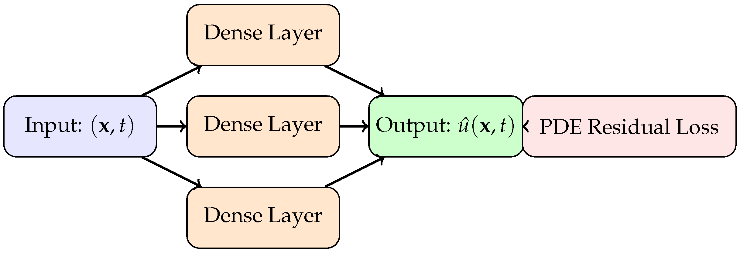
Figure 2.
Training pipeline of a PINN. Training alternates between collocation point sampling, solution prediction, residual computation via automatic differentiation, and weight updates via optimization.
Figure 2.
Training pipeline of a PINN. Training alternates between collocation point sampling, solution prediction, residual computation via automatic differentiation, and weight updates via optimization.
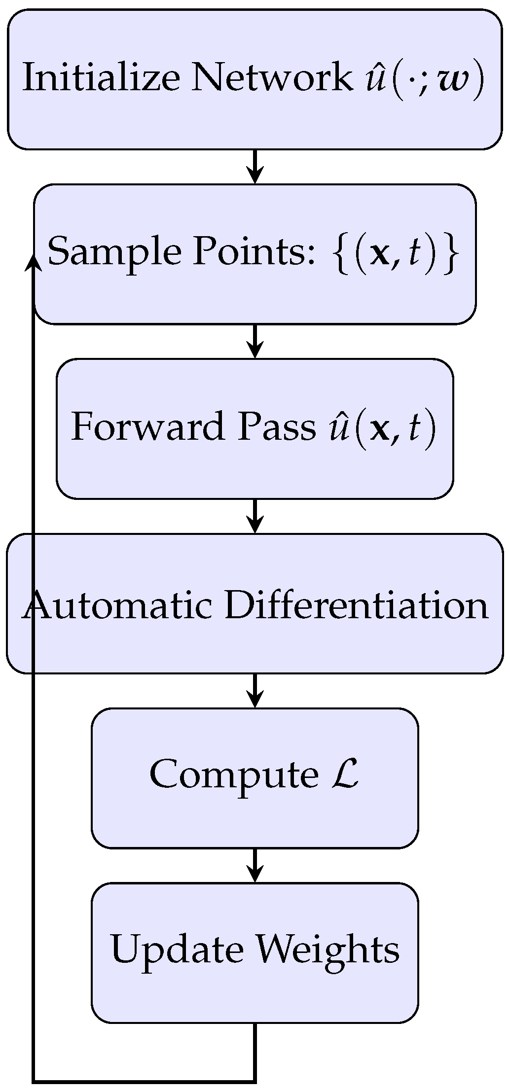
Figure 3.
Application domains of PINNs and associated governing PDEs.
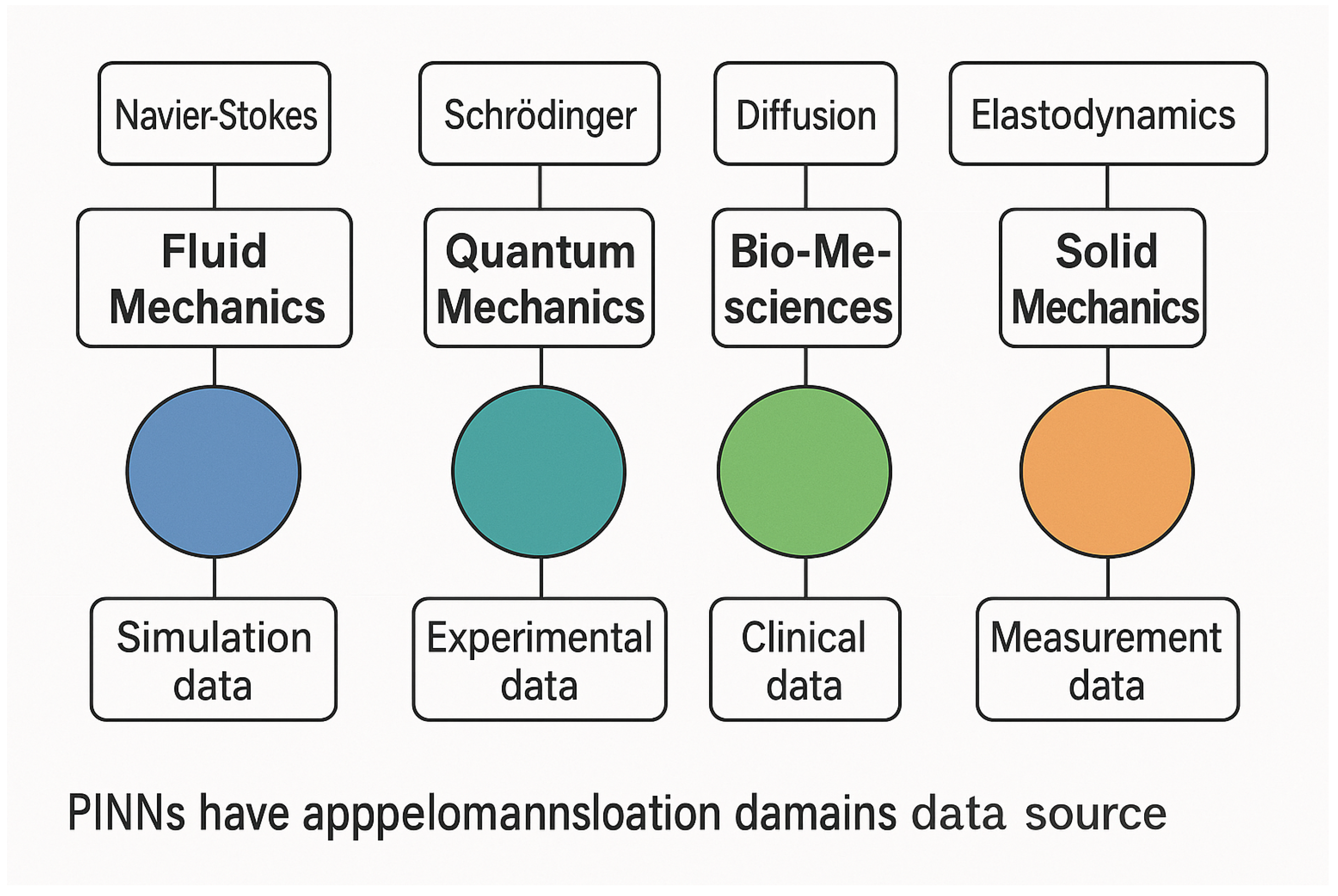
Table 2.
Selected Training Enhancements for PINNs.
| Strategy | Description | Reference |
|---|---|---|
| Adaptive Weighting (NTK, GradNorm) | Dynamically adjusts to balance gradients or curvature. | Wang et al. (2021), Yu et al [28]. (2022) |
| Residual-based Sampling (RAR, AS-PINN) | Selects collocation points based on residual magnitude to improve training focus [29]. | Lu et al. (2021) |
| Curriculum Learning | Trains the model on simpler versions of the PDE before gradually increasing complexity. | Meng et al. (2020) |
| Domain Decomposition (XPINN) | Splits domain into subregions to parallelize and localize training [9]. | Jagtap et al. (2020) |
| Output Normalization | Rescales the PDE solution output for numerical stability during training. | Kissas et al [30]. (2020) |
| Multi-Fidelity Supervision | Combines coarse simulations with high-fidelity data. | Meng et al. (2021) |
Table 3.
Summary of major PINN extensions and their characteristics.
| Extension | Key Feature | Target Problem |
|---|---|---|
| XPINNs | Domain decomposition | Large-scale, multi-physics |
| cPINNs | Integral conservation loss | Conservation laws |
| hpPINNs | Adaptive resolution | Multi-scale problems |
| DeepONets | Operator learning | Parameterized PDEs |
| FNOs | Global convolution in Fourier space | High-resolution spatiotemporal data |
| VPINNs | Variational formulation | Weak-form PDEs |
| Bayesian PINNs | Posterior inference | Uncertainty quantification |
| Multi-modal PINNs | Data fusion from sensors/images | Inverse problems in biomedicine |
Table 4.
Representative benchmark problems in the PINN literature.
| Problem | Equation | Context |
|---|---|---|
| 1D Burgers Equation | Viscous shocks, nonlinearity | |
| 2D Navier–Stokes | Incompressible flow equations | Cylinder flow, cavity flow |
| 1D Heat Equation | Diffusion modeling | |
| Wave Equation | Oscillatory dynamics | |
| Poisson Equation | Electrostatics, steady-state heat | |
| Darcy Flow | Subsurface flow, porous media | |
| Schrödinger Eq. | Quantum systems |
Table 5.
Summary of limitations and open problems in PINNs.
| Category | Limitation / Open Problem |
|---|---|
| Optimization | Stiff PDE loss, imbalance, gradient pathologies |
| Approximation | Difficulty modeling discontinuities or fine scales |
| Scalability | Poor performance on high-dimensional, long-time simulations |
| Data Conflict | Instability due to noisy or conflicting measurements |
| Generalization | Weak transfer to unseen PDEs, geometries, conditions |
| Interpretability | Black-box nature limits scientific insight |
| Deployment | Complex setup and integration into existing workflows |
Disclaimer/Publisher’s Note: The statements, opinions and data contained in all publications are solely those of the individual author(s) and contributor(s) and not of MDPI and/or the editor(s). MDPI and/or the editor(s) disclaim responsibility for any injury to people or property resulting from any ideas, methods, instructions or products referred to in the content. |
© 2025 by the authors. Licensee MDPI, Basel, Switzerland. This article is an open access article distributed under the terms and conditions of the Creative Commons Attribution (CC BY) license (http://creativecommons.org/licenses/by/4.0/).
Copyright: This open access article is published under a Creative Commons CC BY 4.0 license, which permit the free download, distribution, and reuse, provided that the author and preprint are cited in any reuse.


