Solve Bi-Level Optimization Model for Meta-Learning Using Method of Lagrangian Multipliers

1. Introduction

Meta-learning, often referred to as "learning to learn," [1,2,3] has emerged as a powerful framework for improving model generalization, particularly in domains where data distributions vary significantly across tasks.

Inspired by these advances[4], our proposed model integrates task correlation learning directly into the optimization procedure, seeking not only to minimize training loss but also to enhance the quality of downstream decision-making through better generalization. In magnetic resonance imaging (MRI) reconstruction, where datasets can differ widely in anatomy, acquisition protocols, and imaging artifacts, meta-learning provides a promising avenue to build adaptable models. Building on the foundation of optimization-based deep learning methods for MRI reconstruction[5,6] , we propose a bi-level optimization model for meta-learning that explicitly captures the relationship between training and validation datasets through learnable task correlations.

This work is motivated by a line of recent studies exploring optimization-driven and meta-learning approaches, including an optimization-based meta-learning model for diverse datasets[7,8,9] and a learnable variational model for joint multimodal MRI reconstruction and synthesis[10]. These advances illustrate that incorporating optimization formulations into the learning process enhances model robustness across diverse conditions.

Our framework formulates the meta-training as a constrained bi-level optimization problem, where the lower-level problem learns task-specific models weighted by a normalized hyperparameter matrix, and the upper-level problem adjusts these hyperparameters to minimize validation losses. Furthermore, we extend the training dynamics using the method of Lagrangian multipliers (MLM) to provide theoretical equivalence between direct loss minimization and primal-dual optimization updates, following similar optimization principles as used in optimal control frameworks for image processing[11,12].

By synthesizing principles from optimization theory, control dynamics[13], and deep learning, our approach offers a principled and scalable solution for meta-learning training algorithm, potentially improving performance on heterogeneous, real-world imaging datasets. This work continues the trajectory of optimization-based learning[9,12,14].

1.1. Optimization-Based Meta-Learning: Frameworks and Algorithms

In optimization-based meta-learning, the learner is not just learning parameters — it’s learning how to optimize.

Instead of using a fixed optimization method (like SGD or Adam), you train an optimizer (or regularizer) so that across many tasks, it adapts quickly and solves new tasks better. This is typically framed as a bi-level optimization problem:

$$\underset{\theta }{min}{\mathbb{E}}_{\mathcal{T}\sim p\left(\mathcal{T}\right)}\left[{\mathcal{L}}_{\mathrm{meta}}(\theta ;\mathcal{T})\right]$$

where:

• $\theta$ denotes the parameters of the optimizer, model, or regularizer,
• $\mathcal{T}\sim p\left(\mathcal{T}\right)$ represents tasks sampled from a distribution $p\left(\mathcal{T}\right)$,
• ${\mathcal{L}}_{\mathrm{meta}}(\theta ;\mathcal{T})$ measures how well the task is solved after a few optimization steps.

At each meta-training iteration:

• Sample a batch of tasks ${\mathcal{T}}_i$ from the task distribution.
• For each task ${\mathcal{T}}_i$:
  • Initialize model parameters x (e.g., randomly or from a pre-trained model).
  • Inner Loop: Solve the task-specific optimization problem for a few steps using the current optimizer (parameterized by $\theta$), yielding adapted parameters $x_i^{\prime }$.
  • Compute the task loss ${\mathcal{L}}_{\mathrm{task}}(x_i^{\prime };{\mathcal{T}}_i)$.
• Outer Loop:
  • Aggregate all the task losses to compute a meta-loss.
  • Update $\theta$ (the optimizer or model parameters) via gradient descent to improve performance on future tasks.

2. Problem Settings

Suppose we are given a set of N training examples, denoted as ${\left\{({\mathbf{x}}^{\left(j\right)},{\mathbf{u}}^{*\left(j\right)})\right\}}_{j=1}^N$, where for each index $j\in \{1,\dots ,N\}$:

• ${\mathbf{x}}^{\left(j\right)}$ represents the input data (e.g., an undersampled measurement or an input image),
• ${\mathbf{u}}^{*\left(j\right)}$ denotes the corresponding ground-truth output (e.g., a fully sampled or high-quality image).

We aim to train a neural network parameterized by $\mathrm{\Theta }$, where the objective is to learn $\mathrm{\Theta }$ by minimizing a loss function ℓ that measures the discrepancy between the network’s output and the ground truth across the training set.

This training procedure can be formulated as a bilevel optimization problem[15], consisting of two levels:

• Lower-level optimization: For a fixed set of trainable parameters $\mathrm{\Theta }$, we update the reconstruction variable $\mathbf{u}$ by solving a task-specific optimization problem guided by the network.
• Upper-level optimization: After updating $\mathbf{u}$, we update the network parameters $\mathrm{\Theta }$ by minimizing the empirical loss ℓ over the training dataset.

Thus, the network training involves alternating between solving for $\mathbf{u}$ given $\mathrm{\Theta }$, and optimizing $\mathrm{\Theta }$ based on the performance measured by the loss function ℓ.

$$\begin{array}{cc}\hfill \underset{\mathrm{\Theta }}{min}& \ell \left(\mathbf{u}\left(T\right)\right),\hfill \end{array}$$

(1a)

$$\begin{array}{cc}\hfill \mathrm{s}.\mathrm{t}.& \mathbf{u}\left(t\right)=\mathbf{g}(\mathbf{u}(t-1),{\theta }_t),t=1\cdots T,\hfill \end{array}$$

(1b)

$$\begin{array}{cc}\hfill & \mathbf{u}\left(0\right)={\mathbf{u}}_0,\hfill \end{array}$$

(1c)

Set $\mathbf{U}={(\mathbf{u}\left(0\right),\cdots ,\mathbf{u}\left(T\right))}^{⊺}$ and $\mathrm{\Theta }={({\theta }_1,\cdots ,{\theta }_T)}^{⊺}$ be the collection of states $\mathbf{u}\left(t\right)$ and controls ${\theta }_t$ at all time steps respectively. $\mathbf{g}$ is a multi-phase unrolling network inspired by the proximal gradient algorithm, and the output of $\mathbf{g}(·)\in {\mathbb{C}}^{m\times n\times c}$ is the updated multi-coil MRI data from each phase. In our framework, we introduce a neural network $\mathbf{g}$ that serves as an intermediate mapping between consecutive states of the reconstruction variable. Specifically, at each iteration t (where $t=0,\dots ,T-1$), the network $\mathbf{g}$ takes the current estimate ${\mathbf{u}}^{\left(t\right)}$ and produces an updated estimate ${\mathbf{u}}^{(t+1)}$:

$${\mathbf{u}}^{(t+1)}=\mathbf{g}({\mathbf{u}}^{\left(t\right)};\theta \left(t\right)),$$

where $\theta \left(t\right)$ denotes the set of trainable parameters at iteration t.

To initialize the reconstruction process, we define a separate network ${\mathbf{g}}_0$, which operates with an initial set of control parameters $\theta \left(0\right)$. The role of ${\mathbf{g}}_0$ is to map the given partial k-space measurements $\mathbf{f}$ to an initial image reconstruction ${\mathbf{u}}^{\left(0\right)}$:

$${\mathbf{u}}^{\left(0\right)}={\mathbf{g}}_0(\mathbf{f};\theta \left(0\right)).$$

This initial estimate ${\mathbf{u}}^{\left(0\right)}$ then serves as the starting point for the iterative reconstruction process governed by the optimal control system, where $\mathbf{g}$ is applied sequentially to refine the reconstruction across T iterations.

Suppose the training data ${\mathcal{D}}^{tr}={\left\{{\mathcal{D}}_{{\tau }_i}^{tr}\right\}}_{i=1}^{\mathcal{N}}$ which consists of $\mathcal{N}$ batches.

And the validation data ${\mathcal{D}}^{val}={\left\{{\mathcal{D}}_{v_j}^{val}\right\}}_{j=1}^{\mathcal{M}}$ which consists of $\mathcal{M}$ batches.

——————————–

Let $\theta$ be the collection of the network parameters and $\alpha$ be the set of hyper-parameters. We optimize the following bi-level model:

$$\begin{array}{cc}\hfill & \widehat{\alpha }=\underset{\alpha }{arg\; min}\sum _{j=1}^{\mathcal{M}}{\ell }_{v_j}(\theta \left(\alpha \right);{\mathcal{D}}_{v_j}^{val})\hfill \end{array}$$

(2a)

$$\begin{array}{cc}\hfill s.t.& \theta \left(\alpha \right)=\underset{\overline{\theta }}{arg\; min}\sum _{i=1}^{\mathcal{N}}\sigma {\left(\alpha \right)}_i·{\ell }_{{\tau }_i}(\overline{\theta };{\mathcal{D}}_{{\tau }_i}^{tr}),\hfill \end{array}$$

(2b)

$$\begin{array}{cc}\hfill \mathrm{where}& \sum _i\sigma {\left(\alpha \right)}_i=1,0\le \sigma {\left(\alpha \right)}_i\le 1.\hfill \end{array}$$

(2c)

where ℓ denotes the loss function which can be taken as cross entropy loss. And the function $\sigma$ is to normalize the hyperparameter vector $\alpha$, here we can simply take $\sigma$ as the softmax function.

Also we propose a generalized model where $\alpha \in {\mathcal{R}}^{\mathcal{N}\times \mathcal{M}}$, and we denote ${\alpha }_j\in {\mathcal{R}}^{\mathcal{N}}$ denotes the j-th column. After we apply the normalization function $\sigma$ (in (3c)), the matrix $\sigma \left(\alpha \right)$ can be regarded as a weight matrix. Intuitively and ideally, each component $\sigma {\left({\alpha }_j\right)}_i$ can represent the correlation between ${\mathcal{D}}_{{\tau }_i}^{tr}$ and ${\mathcal{D}}_{v_j}^{val}$.

$$\begin{array}{cc}\hfill & \widehat{\alpha }=\underset{\alpha }{arg\; min}\sum _{j=1}^{\mathcal{M}}{\ell }_{v_j}(\theta \left({\alpha }_j\right);{\mathcal{D}}_{v_j}^{val})\hfill \end{array}$$

(3a)

$$\begin{array}{cc}\hfill s.t.& \theta \left({\alpha }_j\right)=\underset{\overline{\theta }}{arg\; min}\sum _{i=1}^{\mathcal{N}}\sigma {\left({\alpha }_j\right)}_i·{\ell }_{{\tau }_i}(\overline{\theta };{\mathcal{D}}_{{\tau }_i}^{tr}),\hfill \end{array}$$

(3b)

$$\begin{array}{cc}\hfill \mathrm{where}& \sum _i\sigma {\left({\alpha }_j\right)}_i=1,0\le \sigma {\left({\alpha }_j\right)}_i\le 1.\hfill \end{array}$$

(3c)

Algorithm 1:

1: Input: Initialize hyper-parameters ${\alpha }^0$ and network parameters ${\theta }^0$. 2: for epoch $p=1,2,\dots ,P$ do 3:    ${\mathit{\theta }}^{\mathit{p}}=\mathbf{a}\mathbf{r}\mathbf{g} {\mathbf{m}\mathbf{i}\mathbf{n}}_{\overline{\mathit{\theta }}}{\sum }_{\mathit{i}=\mathit{1}}^{\mathcal{N}}\mathit{\sigma }{\left({\mathit{\alpha }}^{\mathit{p}-\mathit{1}}\right)}_{\mathit{i}}·{\ell }_{{\mathit{\tau }}_{\mathit{i}}}(\overline{\mathit{\theta }};{\mathcal{D}}_{{\mathit{\tau }}_{\mathit{i}}}^{\mathit{tr}})$⊳ Perform (k steps) gradient update steps in SGD on ${\mathcal{D}}_{{\mathit{\tau }}_{\mathit{i}}}^{\mathit{tr}}$. 4:    ${\mathit{\theta }}_{\mathit{i}}^{\mathit{p}}=\mathbf{a}\mathbf{r}\mathbf{g} {\mathbf{m}\mathbf{i}\mathbf{n}}_{\mathit{\theta }}{\mathit{\alpha }}_{\mathit{i}}^{\mathit{p}-\mathit{1}}·{\ell }_{{\mathit{\tau }}_{\mathit{i}}}(\mathit{\theta },{\mathcal{D}}_{{\mathit{\tau }}_{\mathit{i}}}^{\mathit{tr}})$ 5:    ${\mathit{\alpha }}^{\mathit{p}}=\mathbf{a}\mathbf{r}\mathbf{g} {\mathbf{m}\mathbf{i}\mathbf{n}}_{\mathit{\alpha }}{\sum }_{\mathit{j}=\mathit{1}}^{\mathcal{M}}{\ell }_{{\mathit{v}}_{\mathit{j}}}({\mathit{\theta }}^{\mathit{p}};{\mathcal{D}}_{{\mathit{v}}_{\mathit{j}}}^{\mathit{val}})$     ⊳ Perform gradient update steps in SGD on ${\mathcal{D}}_{{\mathit{v}}_{\mathit{i}}}^{\mathit{val}}$. 6: end for 7: Output: ${\alpha }^P,{\theta }^P$.

3. Network Training from the View of Method of Lagrangian Multipliers (MLM)

The network parameters to be solved from (3) are $\mathrm{\Theta }=\{{\theta }_t:t=1,\cdots T\}$. First, we apply MLM to solve the control problem in Section 2. The Lagrangian of the control problem (3) is

$$\begin{array}{cc}\hfill L(\mathbf{U},\mathrm{\Theta };\mathrm{\Lambda })=\ell \left(\mathbf{u}\left(T\right)\right)& +{\sum }_{t=1}^T\langle {\lambda }_t,\mathbf{u}\left(t\right)-\mathbf{g}(\mathbf{u}(t-1),{\theta }_t)\rangle \hfill \\ \hfill & +\langle {\lambda }_0,\mathbf{u}\left(0\right)-{\mathbf{u}}_0\rangle ,\hfill \end{array}$$

(4)

where $\mathrm{\Lambda }={({\lambda }_0,\cdots ,{\lambda }_T)}^{⊺}$ are Lagrangian multipliers of (3).

We want to find primal solution $({\mathbf{U}}^{*},{\mathrm{\Theta }}^{*})$ and dual solution ${\mathrm{\Lambda }}^{*}$ to solve (3), if $({\mathbf{U}}^{*},{\mathrm{\Theta }}^{*};{\mathrm{\Lambda }}^{*})$ minimize (4), by the first order optimality condition, we have

$$\left\{\begin{array}{}\mathrm{(5a)}& {\partial }_{\mathbf{U}}L({\mathbf{U}}^{*},{\mathrm{\Theta }}^{*};{\mathrm{\Lambda }}^{*})=0\mathrm{(5b)}& {\partial }_{\mathrm{\Theta }}L({\mathbf{U}}^{*},{\mathrm{\Theta }}^{*};{\mathrm{\Lambda }}^{*})=0\mathrm{(5c)}& {\partial }_{\mathrm{\Lambda }}L({\mathbf{U}}^{*},{\mathrm{\Theta }}^{*};{\mathrm{\Lambda }}^{*})=0\end{array}\right.$$

The algorithm is conducted in the following manner:

• Fix $\mathrm{\Theta }$ and define $(\overline{\mathbf{U}},\overline{\mathrm{\Lambda }}):={min}_{\mathbf{U},\mathrm{\Lambda }}L(\mathbf{U},\mathrm{\Theta };\mathrm{\Lambda })$, then by the first order optimality condition of ${\lambda }_t,t=0,\cdots ,T$ we get

  $$\begin{array}{cc}\hfill {\partial }_{{\lambda }_0}\langle {\lambda }_0,\mathbf{u}\left(0\right)-{\mathbf{u}}_0\rangle =0\Rightarrow & \overline{\mathbf{u}}\left(0\right)={\mathbf{u}}_0\hfill \end{array}$$

  (6a)

  $$\begin{array}{cc}\hfill {\partial }_{{\lambda }_t}\langle {\lambda }_t,\mathbf{u}\left(t\right)-\mathbf{g}(\mathbf{u}(t-1),{\theta }_t)\rangle =0\Rightarrow & \overline{\mathbf{u}}\left(t\right)=\mathbf{g}(\overline{\mathbf{u}}(t-1),{\theta }_t),t=1,\cdots ,T,\hfill \end{array}$$

  (6b)

  By the first order optimality condition of $\mathbf{u}\left(t\right),t=1,\cdots ,T$ we get

  $$\begin{array}{cc}\hfill {\partial }_{\mathbf{u}\left(T\right)}[\ell \left(\mathbf{u}\left(T\right)\right)+\langle {\lambda }_T,\mathbf{u}\left(T\right)\rangle ]=0\Rightarrow & {\overline{\lambda }}_T=-{\partial }_{\mathbf{u}\left(T\right)}\ell \left(\overline{\mathbf{u}}\left(T\right)\right),\hfill \end{array}$$

  (7a)

  $$\begin{array}{cc}\hfill {\partial }_{\mathbf{u}\left(t\right)}[\langle {\lambda }_t,\mathbf{u}\left(t\right)\rangle +\langle {\lambda }_{t+1},-\mathbf{g}(\mathbf{u}\left(t\right),{\theta }_{t+1})\rangle ]=0\Rightarrow & {\overline{\lambda }}_t=\langle {\overline{\lambda }}_{t+1},{\partial }_{\mathbf{u}\left(t\right)}\mathbf{g}(\overline{\mathbf{u}}\left(t\right),{\theta }_{t+1})\rangle ,t=1,\cdots ,T-1,\hfill \end{array}$$

  (7b)

  $$\begin{array}{cc}\hfill {\partial }_{\mathbf{u}\left(0\right)}[\langle {\lambda }_0,\mathbf{u}\left(0\right)\rangle +\langle {\lambda }_1,-g(\mathbf{u}\left(0\right),{\theta }_1)\rangle ]=0\Rightarrow & {\overline{\lambda }}_0=\langle {\overline{\lambda }}_1,{\partial }_{\mathbf{u}\left(0\right)}\mathbf{g}(\overline{\mathbf{u}}\left(0\right),{\theta }_1)\rangle .\hfill \end{array}$$

  (7c)

  Therefore for fixed $\mathrm{\Theta }$ we get the optimal solutions $(\overline{\mathbf{U}},\overline{\mathrm{\Lambda }})$ satisfy (1) and (1).
• For fixed $(\mathbf{U},\mathrm{\Lambda })$, we compute the gradient ${\partial }_{\mathrm{\Theta }}L(\mathbf{U},\mathrm{\Theta };\mathrm{\Lambda })$:

  $$\begin{array}{cc}\hfill {\partial }_{\mathrm{\Theta }}L({\mathbf{U}}^k,{\mathrm{\Theta }}^k;{\mathrm{\Lambda }}^k)& =-\langle {\lambda }_0^k,{\partial }_{{\theta }_0}({\mathbf{u}}_k^{\left(0\right)}-{\mathbf{u}}_0^k)\rangle =0,\mathrm{for}t=0.\hfill \end{array}$$

  (8a)

  $$\begin{array}{cc}\hfill {\partial }_{{\theta }_t}L(\mathbf{U},{\theta }_t;\mathrm{\Lambda })& ={\partial }_{{\theta }_t}[-\langle {\lambda }_t,\mathbf{g}(\mathbf{u}(t-1),{\theta }_t)\rangle ]\hfill \end{array}$$

  (8b)

  $$\begin{array}{cc}\hfill & =-\langle {\lambda }_t,{\partial }_{{\theta }_t}\mathbf{g}(\mathbf{u}(t-1),{\theta }_t)\rangle \mathrm{for}t=1,\cdots ,T.\hfill \end{array}$$

  (8c)

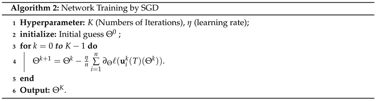
Recall the conventional SGD method, we update ${\mathrm{\Theta }}^{k+1}={\mathrm{\Theta }}^k-{\displaystyle \frac{\eta }{n}}{\displaystyle \sum _{i=1}^n}{\partial }_{\mathrm{\Theta }}\ell \left({\mathbf{u}}_i^k\left(T\right)\left({\mathrm{\Theta }}^k\right)\right)$, where ${\mathbf{u}}^k\left(T\right)$ is interpreted as a function of ${\mathrm{\Theta }}^k={({\theta }_1^k,\cdots ,{\theta }_T^k)}^{⊺}$.

In the following theorem, we show the equivalence between ${\partial }_{\mathrm{\Theta }}L(\overline{\mathbf{U}},\mathrm{\Theta };\overline{\mathrm{\Lambda }})$ and ${\partial }_{\mathrm{\Theta }}\ell \left(\overline{\mathbf{u}}\left(T\right)\left(\mathrm{\Theta }\right)\right)$.

Theorem 1.

${\partial }_{\mathrm{\Theta }}L(\overline{\mathbf{U}},\mathrm{\Theta };\overline{\mathrm{\Lambda }})={\partial }_{\mathrm{\Theta }}\ell \left(\overline{\mathbf{u}}\left(T\right)\left(\mathrm{\Theta }\right)\right)$.

Proof. 

From (6) we have

$$\begin{array}{cc}\hfill {\partial }_{{\theta }_t}\mathbf{g}(\overline{\mathbf{u}}(t-1),{\theta }_t)& ={\partial }_{{\theta }_t}\overline{\mathbf{u}}\left(t\right),t=1,\cdots ,T\hfill \end{array}$$

(9a)

From (7b), we have

$$\begin{array}{cc}\hfill {\overline{\lambda }}_{T-1}& =\langle {\overline{\lambda }}_T,{\partial }_{\mathbf{u}(T-1)}\mathbf{g}(\overline{\mathbf{u}}(T-1),{\theta }_T)\rangle \hfill \end{array}$$

(10a)

$$\begin{array}{cc}\hfill & =\langle -{\partial }_{\mathbf{u}\left(T\right)}\ell \left(\overline{\mathbf{u}}\left(T\right)\right),{\partial }_{\mathbf{u}(T-1)}\overline{\mathbf{u}}\left(T\right)\rangle \mathrm{by}\left(7\mathrm{a}\right),\left(6\mathrm{b}\right)\hfill \end{array}$$

(10b)

$$\begin{array}{cc}\hfill & =-{\partial }_{\mathbf{u}(T-1)}\ell \left(\overline{\mathbf{u}}\left(T\right)\right)\hfill \end{array}$$

(10c)

Similarly, we can show (Section 3) holds for $t=0,\cdots ,T-1$

$${\overline{\lambda }}_t=-{\partial }_{\mathbf{u}\left(t\right)}\ell \left(\overline{\mathbf{u}}\left(T\right)\right),$$

(11)

together with (7a), we have

$${\overline{\lambda }}_t=-{\partial }_{\mathbf{u}\left(t\right)}\ell \left(\overline{\mathbf{u}}\left(T\right)\right),t=0,\cdots ,T.$$

(12)

Hence, (8c) reduces to

$$\begin{array}{cc}\hfill {\partial }_{{\theta }_t}& L(\overline{\mathbf{U}},{\theta }_t;\overline{\mathrm{\Lambda }})=-\langle {\overline{\lambda }}_t,{\partial }_{{\theta }_t}\mathbf{g}(\overline{\mathbf{u}}(t-1),{\theta }_t)\rangle \hfill \end{array}$$

(13a)

$$\begin{array}{cc}\hfill & =\langle {\partial }_{\mathbf{u}\left(t\right)}\ell \left(\overline{\mathbf{u}}\left(T\right)\right),{\partial }_{{\theta }_t}\overline{\mathbf{u}}\left(t\right)\rangle \mathrm{by}\left(12\right),\left(9\mathrm{a}\right)\hfill \end{array}$$

(13b)

$$\begin{array}{cc}\hfill & ={\partial }_{{\theta }_t}\ell \left(\overline{\mathbf{u}}\left(T\right)\left({\theta }_t\right)\right),t=1,\cdots ,T.\hfill \end{array}$$

(13c)

Thus, we derive ${\partial }_{\mathrm{\Theta }}L(\overline{\mathbf{U}},\mathrm{\Theta };\overline{\mathrm{\Lambda }})={\partial }_{\mathrm{\Theta }}\ell \left(\overline{\mathbf{u}}\left(T\right)\left(\mathrm{\Theta }\right)\right)$. □

This theorem shows that applying SGD on the loss function ℓ is equivalent to performing SGD on L. We want to reach the optimal solutions $(\overline{\mathbf{U}},\overline{\mathrm{\Lambda }})$ with fixed $\mathrm{\Theta }$, so we proceed the algorithm to update $\mathrm{\Theta }$ in the iterative scheme by replacing notation $\overline{\mathbf{U}},\overline{\mathrm{\Lambda }}$ as ${\mathbf{U}}^k,{\mathrm{\Lambda }}^k$. This training process is summarized in Algorithm 3, where ${\mathrm{\Lambda }}^k={({\lambda }_0^k,{\lambda }_1^k,\cdots ,{\lambda }_T^k)}^{⊺}$, ${\mathrm{\Theta }}^k={({\theta }_1^k,\cdots ,{\theta }_T^k)}^{⊺}$, and ${\mathbf{U}}^k={({\mathbf{u}}^k\left(0\right),{\mathbf{u}}^k\left(1\right),\cdots ,{\mathbf{u}}^k\left(T\right))}^{⊺}$ for each iteration $k=0,1,\cdots ,K$. Now we can use one step of SGD optimization methods such as ADAM to update $\mathrm{\Theta }$ by replacing ${\partial }_{\mathrm{\Theta }}\ell \left({\mathbf{u}}^k\left(T\right)\left(\mathrm{\Theta }\right)\right)$ to be ${\partial }_{\mathrm{\Theta }}L({\mathbf{U}}^k,\mathrm{\Theta };{\mathrm{\Lambda }}^k)$ with gradient computed in (8).

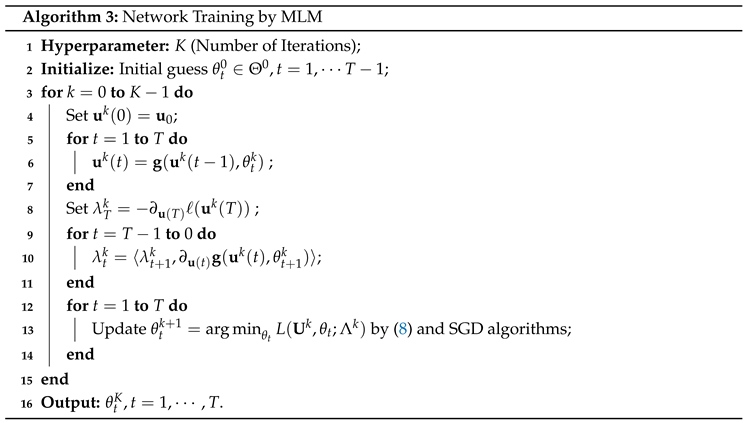
Algorithm 3 trains a meta-learning model by solving a bilevel optimization problem using the Method of Lagrangian Multipliers (MLM).

Instead of naively updating the network parameters by only minimizing the loss, this algorithm:

• Explicitly tracks the primal variables (the reconstruction variables $\mathbf{u}\left(t\right)$),
• And the dual variables (the Lagrange multipliers ${\lambda }_t$),

to ensure that the updates respect the dynamic constraint at each iteration:

$$\mathbf{u}(t+1)=\mathbf{g}(\mathbf{u}\left(t\right),{\theta }_t),$$

where $\mathbf{g}$ denotes the learned update network and ${\theta }_t$ are the trainable control parameters at iteration t.

The forward pass simulates the network behavior over T iterations (like "unrolling" the optimization).

The backward pass computes how the loss at the end depends on every single step (using the chain rule and multipliers). The parameter update ensures that the learned optimizer $\mathbf{g}$ not only reduces loss but respects the dynamic constraints (i.e., how $\mathbf{u}\left(t\right)$ evolves over time).

Thus, it mimics optimal control theory where we treat the evolution of the system as a dynamic process, not just static minimization.

4. Discussion

Optimization is fundamental to solving inverse problems, yet traditional methods often require careful tuning and lack flexibility across domains. Meta-learning addresses this by enabling optimizers to learn from data how to adaptively solve new tasks, capturing task-specific structures, and accelerating convergence[16,17]. This is especially important in applications such as quantitative MRI reconstruction, where diverse data distributions[18] require robust and adaptable optimization strategies.

Optimization and meta-learning are increasingly intertwined with broader developments in decision-making under uncertainty. Recent works in predict-then-optimize frameworks[19], fairness in resource allocation[20], and integrated estimation-optimization perspectives[21] highlight the importance of aligning learning models with downstream optimization goals[22,23,24].

5. Conclusion

In this work, we proposed a bilevel optimization framework for meta-learning, where the training process is viewed through the lens of optimal control theory. By employing the Method of Lagrangian Multipliers (MLM), we explicitly modeled both the primal reconstruction variables and the dual Lagrange multipliers, enabling principled updates that respect the underlying dynamics of the optimization process[25]. Our approach bridges classical optimization techniques with modern deep learning, offering a scalable and theoretically grounded method for learning adaptive optimization strategies.

This formulation not only improves the training stability but also enhances generalization across diverse tasks and domains, making it particularly suitable for challenging inverse problems such as quantitative MRI reconstruction. The equivalence established between direct loss minimization and Lagrangian-based optimization further validates the correctness and efficiency of our method.

Future work will explore extending this framework to more complex scenarios, such as multi-stage reconstruction, uncertainty-aware modeling, and real-time adaptation in dynamic environments. We believe that optimization-driven meta-learning approaches like ours hold strong potential for advancing learning systems in both medical imaging and broader scientific computing domains.

References

- T. M. Hospedales, A. T. M. Hospedales, A. Antoniou, P. Micaelli, and A. J. Storkey, “Meta-learning in neural networks: A survey,” IEEE Transactions on Pattern Analysis and Machine Intelligence, 2021. [CrossRef]
- M. Huisman, J. N. M. Huisman, J. N. van Rijn, and A. Plaat, “A survey of deep meta-learning,” Artificial Intelligence Review, pp. 1–59, 2021. [CrossRef]
- C. Finn, A. C. Finn, A. Rajeswaran, S. Kakade, and S. Levine, “Online meta-learning,” in International Conference on Machine Learning. PMLR, 2019, pp. 1920–1930. [CrossRef]
- W. Bian, Y. W. Bian, Y. Chen, and X. Ye, “An optimal control framework for joint-channel parallel mri reconstruction without coil sensitivities,” Magnetic Resonance Imaging, 2022. [CrossRef]
- D. Kiyasseh, A. D. Kiyasseh, A. Swiston, R. Chen, and A. Chen, “Segmentation of left atrial mr images via self-supervised semi-supervised meta-learning,” in Medical Image Computing and Computer Assisted Intervention–MICCAI 2021: 24th International Conference, Strasbourg, France, –October 1, 2021, Proceedings, Part II 24. Springer, 2021, pp. 13–24. 27 September. [CrossRef]
- W. Bian, A. W. Bian, A. Jang, and F. Liu, “Multi-task magnetic resonance imaging reconstruction using meta-learning,” Magnetic Resonance Imaging, vol. 116, p. 110278, 2025. [CrossRef]
- Y. Chen, C.-B. Y. Chen, C.-B. Schönlieb, P. Liò, T. Leiner, P. L. Dragotti, G. Wang, D. Rueckert, D. Firmin, and G. Yang, “Ai-based reconstruction for fast mri—a systematic review and meta-analysis,” Proceedings of the IEEE, vol. 110, no. 2, pp. 224–245, 2022. [CrossRef]
- W. Bian, Y. W. Bian, Y. Chen, X. Ye, and Q. Zhang, “An optimization-based meta-learning model for mri reconstruction with diverse dataset,” Journal of Imaging, vol. 7, no. 11, p. 231, 2021. [CrossRef]
- Q. Liu, Q. Q. Liu, Q. Dou, and P.-A. Heng, “Shape-aware meta-learning for generalizing prostate mri segmentation to unseen domains,” in Medical Image Computing and Computer Assisted Intervention–MICCAI 2020: 23rd International Conference, Lima, Peru, –8, 2020, Proceedings, Part II 23. Springer, 2020, pp. 475–485. 4 October. [CrossRef]
- W. Bian, Q. W. Bian, Q. Zhang, X. Ye, and Y. Chen, “A learnable variational model for joint multimodal mri reconstruction and synthesis,” in International Conference on Medical Image Computing and Computer-Assisted Intervention. Springer, 2022, pp. 354–364. [CrossRef]
- W. Bian and Y. K. Tamilselvam, “A review of optimization-based deep learning models for mri reconstruction,” AppliedMath, vol. 4, no. 3, pp. 1098–1127, 2024. [CrossRef]
- A. Rajeswaran, C. A. Rajeswaran, C. Finn, S. M. Kakade, and S. Levine, “Meta-learning with implicit gradients,” Advances in neural information processing systems, vol. 32, 2019. [CrossRef]
- S. Wang, J. S. Wang, J. Chen, X. Deng, S. Hutchinson, and F. Dellaert, “Robot calligraphy using pseudospectral optimal control in conjunction with a novel dynamic brush model,” in 2020 IEEE/RSJ International Conference on Intelligent Robots and Systems (IROS). IEEE, 2020, pp. 6696–6703. [CrossRef]
- W. Bian, “Optimization-based deep learning methods for magnetic resonance imaging reconstruction and synthesis,” Ph.D. dissertation, University of Florida, 2022.
- arXiv:2406.02626, 2024.
- Z. Ding, P. Z. Ding, P. Li, Q. Yang, S. Li, and Q. Gong, “Regional style and color transfer,” in 2024 5th International Conference on Computer Vision, Image and Deep Learning (CVIDL). IEEE, 2024, pp. 593–597. [CrossRef]
- W. Bian, A. W. Bian, A. Jang, L. Zhang, X. Yang, Z. Stewart, and F. Liu, “Diffusion modeling with domain-conditioned prior guidance for accelerated mri and qmri reconstruction,” IEEE Transactions on Medical Imaging, 2024. [CrossRef]
- Z. Ke, S. Z. Ke, S. Zhou, Y. Zhou, C. H. Chang, and R. arXiv preprint arXiv:2501.07033, arXiv:2501.07033, 2025.
- S. Verma, Y. S. Verma, Y. Zhao, S. Shah, N. Boehmer, A. Taneja, and M. Tambe, “Group fairness in predict-then-optimize settings for restless bandits,” in The 40th Conference on Uncertainty in Artificial Intelligence.
- N. Boehmer, Y. N. Boehmer, Y. Zhao, G. Xiong, P. Rodriguez-Diaz, P. D. C. Cibrian, J. Ngonzi, A. Boatin, and M. Tambe, “Optimizing vital sign monitoring in resource-constrained maternal care: An rl-based restless bandit approach,” in Proceedings of the AAAI Conference on Artificial Intelligence, vol. 39, no. 28, 2025, pp. 28 843–28 849. [CrossRef]
- A. N. Elmachtoub, H. A. N. Elmachtoub, H. Lam, H. Zhang, and Y. arXiv preprint arXiv:2304.06833, arXiv:2304.06833, vol. 107, 2023.
- W. Bian, P. W. Bian, P. Li, M. Zheng, C. Wang, A. Li, Y. Li, H. Ni, and Z. Zeng, “A review of electromagnetic elimination methods for low-field portable mri scanner,” in 2024 5th International Conference on Machine Learning and Computer Application (ICMLCA). IEEE, 2024, pp. 614–618. [CrossRef]
- Z. Li, S. Z. Li, S. Qiu, and Z. Ke, “Revolutionizing drug discovery: Integrating spatial transcriptomics with advanced computer vision techniques,” in 1st CVPR Workshop on Computer Vision For Drug Discovery (CVDD): Where are we and What is Beyond?
- Z. Ke and Y. Yin, “Tail risk alert based on conditional autoregressive var by regression quantiles and machine learning algorithms,” in 2024 5th International Conference on Artificial Intelligence and Computer Engineering (ICAICE). IEEE, 2024, pp. 527–532. [CrossRef]
- W. Bian, A. W. Bian, A. Jang, and F. Liu, “Improving quantitative mri using self-supervised deep learning with model reinforcement: Demonstration for rapid t1 mapping,” Magnetic Resonance in Medicine, vol. 92, no. 1, pp. 98–111, 2024. [CrossRef]
Disclaimer/Publisher’s Note: The statements, opinions and data contained in all publications are solely those of the individual author(s) and contributor(s) and not of MDPI and/or the editor(s). MDPI and/or the editor(s) disclaim responsibility for any injury to people or property resulting from any ideas, methods, instructions or products referred to in the content. |
© 2025 by the authors. Licensee MDPI, Basel, Switzerland. This article is an open access article distributed under the terms and conditions of the Creative Commons Attribution (CC BY) license (http://creativecommons.org/licenses/by/4.0/).
Copyright: This open access article is published under a Creative Commons CC BY 4.0 license, which permit the free download, distribution, and reuse, provided that the author and preprint are cited in any reuse.