Submitted:
25 April 2025
Posted:
28 April 2025
You are already at the latest version
Abstract
This paper presents a learning-assisted approach for state estimation of quadruped robots using observations of proprioceptive sensors including multiple inertial measurement units (IMUs). Specifically, one body IMU and four additional IMUs attached to each calf link of the robot are used for sensing the dynamics of the body and legs, in addition to joint encoders. The extended Kalman filter (EKF) is employed to fuse sensor data to estimate the robot’s states in the world frame and enhance the convergence of EKF. To circumvent the requirements for the measurements from the motion capture (mocap) system or other vision systems, the right-invariant EKF (RI-EKF) is extended to employ the foot IMU measurements for enhanced state estimation, and a learning-based approach is presented to estimate the vision system measurements for the EKF. 1D convolutional neural networks (CNN) are leveraged to estimate required measurements using only the available proprioception data. Experiments on the real data of a quadruped robot demonstrate that proprioception can be sufficient for state estimation, and the proposed learning-assisted approach without using data from vision systems can achieve competitive accuracy compared to EKF using the mocap measurements and smaller estimation errors than RI-EKF using multi-IMU measurements.
Keywords:
Learning-assisted extended Kalman filter
; invariant extended Kalman filter
; proprioceptive state estimation
1. Introduction
Accurate state estimation is critical for balance and motion planning of quadruped robots on challenging terrains. The requirements of real-time implementation and high accuracy for state estimation in the real world restrict the sensor and algorithm selection [1].
Exteroception and proprioception are two distinct sensory modalities that play crucial roles in state estimation for legged robots [2]. While exteroception has been investigated for state estimation with external environment information from sensors such as cameras [3] and lidars [4], exteroceptive sensors may be prone to environmental disturbances and perceptual limitations (e.g., occlusions, varying lighting conditions), and provide large amounts of high-dimension sensory data that can be computationally demanding for real-time processing, which limits its applicability. Instead, proprioception involves sensing the internal state of the robot, including internal sensors like joint encoders, force sensors, and inertial measurement units (IMUs) that provide immediate feedback about the robot’s position, orientation, and internal forces in real time. Proprioceptive state estimation has become a popular design due to its low latency, high energy efficiency, and low computational demands [5]. The challenges of proprioceptive state estimation lie in calibration, drift, and sensor noise.
Extended Kalman filter (KF) is a commonly used approach for sensor fusion and state estimation [6,7]. EKF integrates measurements from multiple sensors (e.g., encoders, IMUs) with the robot’s motion model to estimate the state variables while considering measurement noise and uncertainties. Bloesch et al. [8] presented a consistent fusion of leg kinematics and IMU using an observability-constrained EKF for state estimation. Furthermore, Yang et al. [9] proposed online kinematic calibration for legged robots to reduce the velocity estimation errors caused by inaccurate leg-length knowledge. Then, Multi-IMU Proprioceptive Odometry (MIPO) [10] was developed to improve upon KF-based Proprioceptive Odometry (PO) methods that only use a single IMU. It is noted that MIPO focuses on PO rather than the full state estimation and uses the mocap system for measuring the body yaw. However, EKF is capable of diverging in some challenging situations. Invariant EKF (IEKF) has been increasingly investigated to enhance convergence of state estimation. The state is defined on a Lie group and dynamics satisfy a particular group-affine property in IEKF. The invariance of the estimation error with respect to a Lie group action leads to the estimation error satisfying a log-linear autonomous differential equation on the Lie algebra, allowing the design of a nonlinear state estimator with strong convergence properties. Hartley et al. [11] derived an IEKF for a system containing IMU and contact sensor dynamics, with forward kinematic correction measurements. However, few works consider the IEKF for multi-IMU proprioceptive state estimation in the context of quadruped robots. Xavier et al. [12] considered multiple IMUs distributed throughout the robot’s structure for state estimation of humanoid robots. In this work, we extend IEKF for state estimation of a quadruped robot with a body IMU and four foot IMUs, which makes a good benchmark.
Moreover, machine learning has been employed to address the challenges of proprioceptive state estimation. In particular, learning-based approaches have been developed for reliable contact detection and measurements estimation with reduced sensor demands under challenging scenarios. Lin et al. [13] developed a learning-based contact estimator for IEKF to bypass the need for physical contact sensors. Buchanan et al. [14] proposed a learned inertial displacement measurement to improve state estimation in challenging scenarios where leg odometry is unreliable, such as slipping and compressible terrains. Teng et al. [15] proposed a neural measurement network (NMN) to estimate the contact probabilities of feet and the body linear velocity for IEKF. The inputs to the NMN consist of current body acceleration, body angular velocity, joint angles, joint velocities, and previous positional joint targets. Moreover, Liu et al. [16] employed a physics-informed neural network in conjunction with an unscented KF using proprioceptive sensory data to enhance the state estimation process. Inspired by the previous works, this paper aims to develop an accurate full-state estimator using only proprioceptive information. In particular, built upon the MIPO, we use a 1D CNN learned from multi-IMU and other internal sensor data with groundtruth body orientations to estimate the body yaw, to avoid the mocap or sophisticated visual-inertial-leg odometry algorithm (e.g., [17]) for accurate yaw measurements/estimates. Then, the yaw angles predicted by the CNN model are used by EKF to estimate states. Furthermore, we compare this learning-assisted EKF approach with the IEKF using multi-IMU measurements.
The main contribution of this paper lies in presenting a learning-assisted multi-IMU proprioceptive state estimation (LMIPSE) approach that provides accurate full-state estimation using only proprioception. The remainder of the paper is organized as follows: Section 2 provides the problem formulation and related preliminaries; Section 3 presents the right-invariant EKF (RI-EKF) using multi-IMU measurements; Section 4 presents the proposed LMIPSE; Section 5 provides experimental results; and finally, Section 6 summarizes this paper.
2. Problem Formulation and Related Preliminaries
The states to estimate for a quadruped robot include the orientation , velocity , and position of the body in the world frame W. The sensor measurements considered for updating state estimations in this paper are from 5 IMUs and 4 joint encoders. We use to denote the body IMU frame which is aligned with the body frame B and use to denote the frames of the IMUs attached to the legs. Additionally, denotes the frames of the foot-end contact points and correspond to the front left, front right, hind left, and hind right foot, respectively.
2.1. Measurements and System Model
Consider the IMU measurements model described by
where , , and denote the measurement, bias, and white Gaussian noise of the gyroscope in the i-th IMU, respectively; , , and denote the measurement, bias, and white Gaussian noise of the accelerometer in the i-th IMU, respectively; Eq. (1c) considers random walk model of the bias terms of the IMU, and and are white Gaussian noise. Given the angular velocity and linear acceleration measured by the body IMU as well as the contacts to the ground and the joint positions from the joint encoders, the system model can be described by
where denotes a skew symmetric matrix; is the gravity vector; is the position of the i-th contact point in the world frame; with and denoting the location of the i-th contact point in the body frame. It is noted that Eq. (2d) assumes zero measured velocity for the contact point.
2.2. Right-Invariant EKF
The right-invariant EKF (RI-EKF) has proven consistent in orientation estimation by maintaining the structure of the orientation space and effective in drift mitigation by properly propagating uncertainties through the state space [18]. The RI-EKF for one body IMU and the contact process model with a forward kinematics measurement model has been derived in [11,19]. The prediction step and the update step of the RI-EKF are as follows.
2.2.1. Prediction Step
Assuming zero-order hold to the input and performing Euler integration from time to , the discrete dynamics are described by
where , denotes the corrected estimation with all the measurements until and denotes the one-step-ahead prediction using the dynamic model with the corrected estimates at ; is the discrete state transformation matrix with and
being the system matrix of the linearized right-invariant error dynamics; the estimation error with and ; with and
is the matrix exponential; denotes the adjoint map and is the associated element in a matrix Lie group for .
2.2.2. Update Step
where
is the embedding of the states in the matrix Lie group1; is the correction term with K being the Kalman gain and for selecting the first three rows of the right-hand-side matrix. The Kalman gain is given by
where is the covariance matrix of the additive white Gaussian noise from the leg kinematics measurements.
2.3. Multi-IMU Proprioceptive Odometry
Multiple IMUs, including body and foot IMUs, have been used with joint encoders for legged robots to achieve low-drift long-term position and velocity estimation using an EKF. The foot IMUs can address the limitations of the PO using the single body IMU by enabling the updates of the foot positions during the airborne phase and considering the rolling during the contact without the zero-velocity assumption for the Leg Odometry velocity. In particular, foot IMU data was employed to update foot velocities in the prediction step and determine foot contact models and slip for the measurement model [10]. The process model for MIPO is
where originates from the derivative of with , , denoting the roll, pitch, and yaw angles, respectively. The measurement model is
where the last term is based on the pivoting model [10]; × denotes the cross product of two vectors; ; using to denote the distance between the foot center and the foot surface and to denote the contact normal vector expressed in the world frame, is the pivoting vector pointing from the contact point to the body center. The last term in (8) can be used for the update step only when a foot is in contact with the ground. To detect the contact and slip, a statistical test based on Mahalanobis distance is used in [10] as follows:
where and is the covariance matrix of z estimated by the EKF; is the hypothesis testing threshold. The foot is recognized as being in non-slipping contact if (9) is satisfied. Since RI-EKF shows superior performance, we will present the RI-EKF approach for state estimation using multi-IMU measurements.
3. RI-EKF Using Multi-IMU Measurements
In this section, we present RI-EKF using multi-IMU measurements as a strong benchmark. Considering the linear velocity of the foot as a state in the system dynamics, the augmented robot state where denotes the linear velocity of the foot i contact foot in the world frame and . Then, we consider
The foot IMUs can provide the estimation of the foot velocities and accelerations even during slipping by
Consequently, we have
with . The right-invariant error between two trajectories and is defined as
where maps a vector to the corresponding element of the Lie algebra. The can be shown to satisfy the group affine property. Therefore, the right-invariant error dynamics are trajectory independent and satisfy [18]. Considering the IMU biases,
where and . To let the invariant error satisfy the log-linear property [18], is defined by . Using the first-order approximation , we can have
with . The covariance matrix of the process noise for the augmented error dynamics is .
Using the measurements of the gyroscope on the foot i,
where . can be expressed in the right-invariant observation structure in [18] as follows
Then,
where denotes the block diagonal operation, incorporates the uncertainty in encoder measurements, kinematic model, the effect of slip and gyroscope bias [19], and represents the noise of the measured velocity for the i-th contact point.
4. Learning-Assisted Multi-IMU Proprioceptive State Estimation
A notable limitation of MIPO [10] arises from its reliance on yaw angle measurements provided by a motion capture system. This dependency arises because using motion capture data significantly enhances the accuracy of the state estimation model. However, solely relying on IMU measurements or EKF predictions results in poor accuracy due to the high noise levels in IMU data and the lack of a cross-referencing method to correct these measurements. This reliance on motion capture systems, which are typically unavailable in outdoor environments or general experimental setups, limits the model’s applicability. To address this limitation, our method employs a learning-based approach to predict yaw angles from available data sources, including IMUs, joint motor encoders, and foot contact sensors. This predictive capability enables the replacement of direct motion capture measurements, thus fitting seamlessly within the multi-IMU odometry framework and broadening the model’s applicability to outdoor and less controlled environments. Figure 1 shows the schematic of our proposed LMIPSE.
To train a model for predicting yaw angles online, we first collect a dataset denoted by where are the inputs of the model while is the output the model learns to predict, is the foot force sensor measurements, is the time window size, and is the data set size. The dataset can be randomly split into a training set and a testing set . It is noted that mocap is only needed for collecting the data of but is needless for state estimation. Many model architectures have been proposed for signal processing, and we consider a 1D version of the ResNet (ResNet1D) which has proven efficient in learning inertial odometry [14,20]. Then, the ResNet1D denoted by with parameters w can be trained by minimizing the following Smooth L1 loss (aka Huber Loss)
The Huber loss (22) is chosen for its robustness to outliers in data. It smoothly transitions to a linear loss for errors larger than a certain threshold . This combination of the squared loss and the absolute loss allows the Huber loss to provide the benefits of both types of losses.
It is noted that NN design significantly affects the generalization of the data-driven models [21]. Besides directly predicting yaw angles, we consider using a NN denoted by to model the mismatch between the yaw data () from the mocap system and the yaw estimates () by the body IMU dead reckoning (DK). To learn an accurate , first, we transform the dataset into where with denoting the estimated yaw angle by body IMU DK. Then, we optimize in by minimizing on the transformed dataset .
After finding a model that achieves small testing errors on , we use the model to predict the correction factor for the yaw angle online. The predicted correction factor is then added to the yaw estimate of IMU DK to obtain the final corrected yaw angle prediction . The corrected is used for the prediction step and update step of the EKF. Specifically, at time instant k, the prediction step is
where with denoting the state transition function in (7), with denoting the process noise in (7), and is the covariance matrix of ; the update step is
where , and .
5. Experiments and Validation
This section validates the proposed learning-assisted multi-imu proprioceptive state estimation approach using simulation and real data of a legged robot.
5.1. Dataset Description
The dataset utilized for this study was collected using a Unitree Go 1 robot in a lab space equipped with a highly accurate mocap system, as detailed in the work [10]. The robot was equipped with several proprioceptive sensors, including a body MEMS IMU, twelve joint motor encoders, and four foot pressure contact sensors. An MPU9250 IMU was also mounted on each robot foot to capture additional inertial information.
During indoor trials, the robot operated on flat ground and moved at speeds ranging from 0.4 to 1.0 m/s. Sensor data, including linear accelerations and angular velocities from the IMUs, torque and angle measurements from the joint motor encoders, and orientation data and positional data from the motion capture system. To ensure consistency, all collected data were first resampled to the same frequency, aligned to the same start and end times, and normalized such that the starting location of the robot was at the origin. These data were stored in a rosbag file and are publicly available [10].
A key limitation of the dataset is its short duration of approximately 45 seconds and the simple flat terrain of the testing environment, which might not significantly affect the IMU data’s susceptibility to drift. To address these limitations and simulate a more practical scenario, Gaussian noise and a time-integrated Gaussian noise drift were added to the body IMU data. This setup was intended to assess the robustness of the state estimation algorithms under conditions that more closely mimic operational environments with potential IMU data degradation.
5.2. Experimental Setup
In our study, the mocap system’s pose measurements serve as the ground truth, providing a high-fidelity benchmark for evaluating the performance of various state estimation methods. The Multi-IMU Proprioceptive Odometry (MIPO), which integrates multiple IMUs mounted on the robot’s feet, serves as the baseline against which other methods are compared. Additionally, we explore the body IMU dead reckoning as a first baseline method, where angular velocity measurements are integrated over time to estimate orientation. However, due to IMU drift, this method typically yields less reliable results.
Impacts of NN Design
To address the limitations caused by dataset variability and enhance the model’s generalizability across different robotic movements, we implemented two CNN-based approaches based on a 1D ResNet architecture [22]. The first approach is the Multi-IMU CNN Angle Estimator (MI-CAE), which predicts yaw angles directly, using mocap-derived orientation measurements as ground truth. The second approach is the Multi-IMU CNN angle Correction Enhancer (MI-CCE), which aims to predict a correction factor for the IMU-derived yaw angles, with the ground truth being the discrepancy between the IMU dead reckoning and mocap measurements. The corrected yaw angles are then integrated into the MIPO framework to enhance state estimation. The efficacy of these approaches is subsequently evaluated by comparing the resulting position estimates against the mocap system data, thus ensuring a robust assessment of each approach’s ability to improve upon traditional IMU dead reckoning techniques in dynamic environments.
NN architecture: We used a ResNet1D as the backbone of the model for processing sensor data. The ResNet1D structure comprises 9 residual blocks, each containing a sequence of convolutional layers, batch normalization, and ReLU activation functions. The output of the model is configured to produce a single continuous value, which presents the predicted yaw angles or the correction factor for IMU yaw angle measurements. Table 1 summarizes the architecture of the ResNet1D model.
Training settings: From a training perspective, the model employs the Adam optimizer with an initial learning rate of 0.001 and a weight decay of 0.001 to prevent overfitting. Additionally, a ReduceLROnPlateau learning rate scheduler is integrated to adjust the learning rate based on the performance, specifically reducing the rate if no improvement in loss is observed over 10 epochs. This is complemented by using Huber Loss as the loss function. The entire model is trained for 50 epochs.
5.3. Results and Discussions
5.3.1. Yaw Prediction Model
Table 2 summarizes the testing accuracy of the two CNN-based models using different training set sizes. After experimenting with various sizes, we chose to use 3000 random data points to balance performance and generalization.
Furthermore, Figure 2 compares the yaw prediction results of MI-CAE and MI-CCE, demonstrating that MI-CCE achieved smaller prediction errors. Since the yaw predictions are used for EKF, we further tested the performance of the two models for state estimation.
5.3.2. Proprioceptive State Estimation
We assessed the performance of different state estimation methods under both low-noise and high-noise conditions. Low Noise Condition refers to the original IMU data measured using a high-quality IMU in a controlled lab environment. High Noise Condition is created by adding Gaussian noise and drift to the IMU measurements to mimic the unstable environment.
Table 3 summarizes the results of various state estimation methods under low IMU noise conditions. The MIPO method [10] achieves significantly higher positioning accuracy compared to SIPO. However, using yaw angles estimated by EKF rather than motion capture (mocap) measurements substantially increases the position estimation errors for both SIPO and MIPO. When using the body IMU dead reckoning (DK) method, the performance of MIPO with mocap is slightly degraded, and this degradation compounds over time. The MIPSE with RI-EKF reduces estimation errors but still results in much larger errors compared to MIPO using mocap. In contrast, the MI-CAE method uses CNN-predicted yaw angles derived from multiple IMU measurements for state estimation. This results in an average drift of 15.65%, a median drift of 15.87%, an RMSE of 0.304946, and a maximum RSE of 0.855203. The MI-CCE method improves upon MI-CAE by using a CNN to predict an angle correction factor from multiple IMU measurements, which is then used to correct the IMU data before performing state estimation. This method shows slightly lower drift percentages and error metrics, with an average drift of 15.65%, a median drift of 15.87%, an RMSE of 0.304946, and a maximum RSE of 0.855203. The discrepancy in state estimation performance is smaller than the difference in yaw prediction accuracy between MI-CAE and MI-CCE, demonstrating that prediction errors can be mitigated by the EKF.
Notably, while the MIPO method uses angle information from a motion capture system and achieves the lowest error metrics, the CNN-enhanced methods, MI-CAE and MI-CCE, exhibit similar levels of accuracy without the reliance on external motion capture systems.
Table 4 summarizes the results of various state estimation methods under high IMU noise. Our LMIPSE using CCE achieved the best results regarding all three performance measurements. Furthermore, LMIPSE is more robust to increased noise level than MIPO with DK, as the median drift was increased only by 0.03% for LMIPSE as compared to 0.25% for MIPO with DK. Additionally, Figure 3 compares the trajectory estimation, and Figure 4 compares the state estimation results of LMIPSE and other methods.
6. Concluding Remarks
A learning-assisted EKF approach was presented for multi-IMU proprioceptive state estimation of quadruped robots. In particular, a 1D CNN-based model for estimating the measurements required for EKF was trained offline using the ground-truth measurements from the mocap system and the buffers of proprioception data (including IMUs and joint encoders measurements). Then, the trained model was used to estimate the measurements online for EKF. Experiments demonstrated that the proposed approach improved the accuracy of the state estimation as compared to multi-IMU state estimation using RI-EKF and proprioceptive odometry without using multiple IMUs. In future work, we will consider learning-based approaches for tuning the hyperparameters of the filters [23].
Author Contributions
Conceptualization, X.L., Y.B. and H.X.; methodology, Y.B. and Z.F.; software, X.L. and Y.B.; validation, X.L. and Y.B.; formal analysis, X.L. and Y.B.; investigation, P.C. and D.S.; resources, G.C.; data curation, X.L. and Y.B.; writing—original draft preparation, X.L. and Y.B.; writing—review and editing, P.C.; visualization, X.L. and Y.B.; supervision, P.C., D.S. and G.C.; project administration, D.S. and G.C.; funding acquisition, D.S. and G.C. All authors have read and agreed to the published version of the manuscript.
Data Availability Statement
The raw data supporting the conclusions of this article will be made available by the authors on request.
Conflicts of Interest
The authors declare no conflicts of interest.
References
- Bloesch, M. State estimation for legged robots-kinematics, inertial sensing, and computer vision. PhD thesis, ETH Zurich, 2017.
- Nobili, S.; Camurri, M.; Barasuol, V.; Focchi, M.; Caldwell, D.; Semini, C.; Fallon, M. Heterogeneous sensor fusion for accurate state estimation of dynamic legged robots. In Proceedings of the Robotics: Science and System XIII, 2017.
- Bloesch, M.; Burri, M.; Omari, S.; Hutter, M.; Siegwart, R. Iterated extended Kalman filter based visual-inertial odometry using direct photometric feedback. The International Journal of Robotics Research 2017, 36, 1053–1072. [Google Scholar] [CrossRef]
- Zhao, S.; Zhang, H.; Wang, P.; Nogueira, L.; Scherer, S. Super odometry: Imu-centric lidar-visual-inertial estimator for challenging environments. In Proceedings of the 2021 IEEE/RSJ International Conference on Intelligent Robots and Systems (IROS). IEEE, 2021, pp. 8729–8736. [CrossRef]
- Fink, G.; Semini, C. Proprioceptive sensor fusion for quadruped robot state estimation. In Proceedings of the 2020 IEEE/RSJ International Conference on Intelligent Robots and Systems (IROS). IEEE, 2020, pp. 10914–10920. [CrossRef]
- Ribeiro, M.I. Kalman and extended kalman filters: Concept, derivation and properties. Institute for Systems and Robotics 2004, 43, 3736–3741. [Google Scholar]
- Bao, Y.; Shen, D.; Chen, G.; Pham, K.; Blasch, E. Resilient Range-Only Cooperative Positioning of Multiple Smart Unmanned Aerial Systems. In Proceedings of the International Conference on Security and Privacy in Cyber-Physical Systems and Smart Vehicles. Springer, 2023, pp. 130–147. [CrossRef]
- Bloesch, M.; Hutter, M.; Hoepflinger, M.A.; Leutenegger, S.; Gehring, C.; Remy, C.D.; Siegwart, R. State estimation for legged robots-consistent fusion of leg kinematics and IMU. Robotics 2013, 17, 17–24. [Google Scholar]
- Yang, S.; Choset, H.; Manchester, Z. Online kinematic calibration for legged robots. IEEE Robotics and Automation Letters 2022, 7, 8178–8185. [Google Scholar] [CrossRef]
- Yang, S.; Zhang, Z.; Bokser, B.; Manchester, Z. Multi-IMU Proprioceptive Odometry for Legged Robots. In Proceedings of the 2023 IEEE/RSJ International Conference on Intelligent Robots and Systems (IROS). IEEE, 2023, pp. 774–779.
- Hartley, R.; Jadidi, M.G.; Grizzle, J.W.; Eustice, R.M. Contact-aided invariant extended Kalman filtering for legged robot state estimation. arXiv preprint arXiv:1805.10410 2018. [CrossRef]
- Xavier, F.E.; Burger, G.; Pétriaux, M.; Deschaud, J.E.; Goulette, F. Multi-IMU Proprioceptive State Estimator for Humanoid Robots. In Proceedings of the 2023 IEEE/RSJ International Conference on Intelligent Robots and Systems (IROS). IEEE, 2023, pp. 10880–10887. [CrossRef]
- Lin, T.Y.; Zhang, R.; Yu, J.; Ghaffari, M. Legged Robot State Estimation using Invariant Kalman Filtering and Learned Contact Events. In Proceedings of the Conference on Robot Learning. PMLR, 2022, pp. 1057–1066.
- Buchanan, R.; Camurri, M.; Dellaert, F.; Fallon, M. Learning inertial odometry for dynamic legged robot state estimation. In Proceedings of the Conference on robot learning. PMLR, 2022, pp. 1575–1584.
- Youm, D.; Oh, H.; Choi, S.; Kim, H.; Hwangbo, J. Legged Robot State Estimation With Invariant Extended Kalman Filter Using Neural Measurement Network. arXiv preprint arXiv:2402.00366 2024. [CrossRef]
- Liu, Y.; Bao, Y.; Cheng, P.; Shen, D.; Chen, G.; Xu, H. Enhanced robot state estimation using physics-informed neural networks and multimodal proprioceptive data. In Proceedings of the Sensors and Systems for Space Applications XVII. SPIE, 2024, Vol. 13062, pp. 144–160. [CrossRef]
- Yang, S.; Zhang, Z.; Fu, Z.; Manchester, Z. Cerberus: Low-drift visual-inertial-leg odometry for agile locomotion. In Proceedings of the 2023 IEEE International Conference on Robotics and Automation (ICRA). IEEE, 2023, pp. 4193–4199. [CrossRef]
- Barrau, A.; Bonnabel, S. The invariant extended Kalman filter as a stable observer. IEEE Transactions on Automatic Control 2016, 62, 1797–1812. [Google Scholar] [CrossRef]
- Teng, S.; Mueller, M.W.; Sreenath, K. Legged robot state estimation in slippery environments using invariant extended kalman filter with velocity update. In Proceedings of the 2021 IEEE International Conference on Robotics and Automation (ICRA). IEEE, 2021, pp. 3104–3110. [CrossRef]
- Liu, W.; Caruso, D.; Ilg, E.; Dong, J.; Mourikis, A.I.; Daniilidis, K.; Kumar, V.; Engel, J. TLIO: Tight Learned Inertial Odometry. IEEE Robotics and Automation Letters 2020, 5, 5653–5660. [Google Scholar] [CrossRef]
- Bao, Y.; Thesma, V.; Kelkar, A.; Velni, J.M. Physics-guided and Energy-based Learning of Interconnected Systems: from Lagrangian to Port-Hamiltonian Systems. In Proceedings of the 2022 IEEE 61st Conference on Decision and Control (CDC), 2022, pp. 2815–2820. [CrossRef]
- Hong, S.; Xu, Y.; Khare, A.; Priambada, S.; Maher, K.; Aljiffry, A.; Sun, J.; Tumanov, A. HOLMES: Health OnLine Model Ensemble Serving for Deep Learning Models in Intensive Care Units. In Proceedings of the Proceedings of the Proceedings of the 26th ACM SIGKDD International Conference on Knowledge Discovery & Data Mining, 2020, pp. 1614–1624. [CrossRef]
- Fan, Z.; Shen, D.; Bao, Y.; Pham, K.; Blasch, E.; Chen, G. RNN-UKF: Enhancing Hyperparameter Auto-Tuning in Unscented Kalman Filters through Recurrent Neural Networks. In Proceedings of the The 27th International Conference on Information Fusion. IEEE, 2024, pp. 1–8. [CrossRef]
| 1 | Without loss of generality, we will give all further equations assuming only a single contact point, as the process and measurement models are identical for each contact point. |
Figure 1.
The schematic of our proposed LMIPSE.
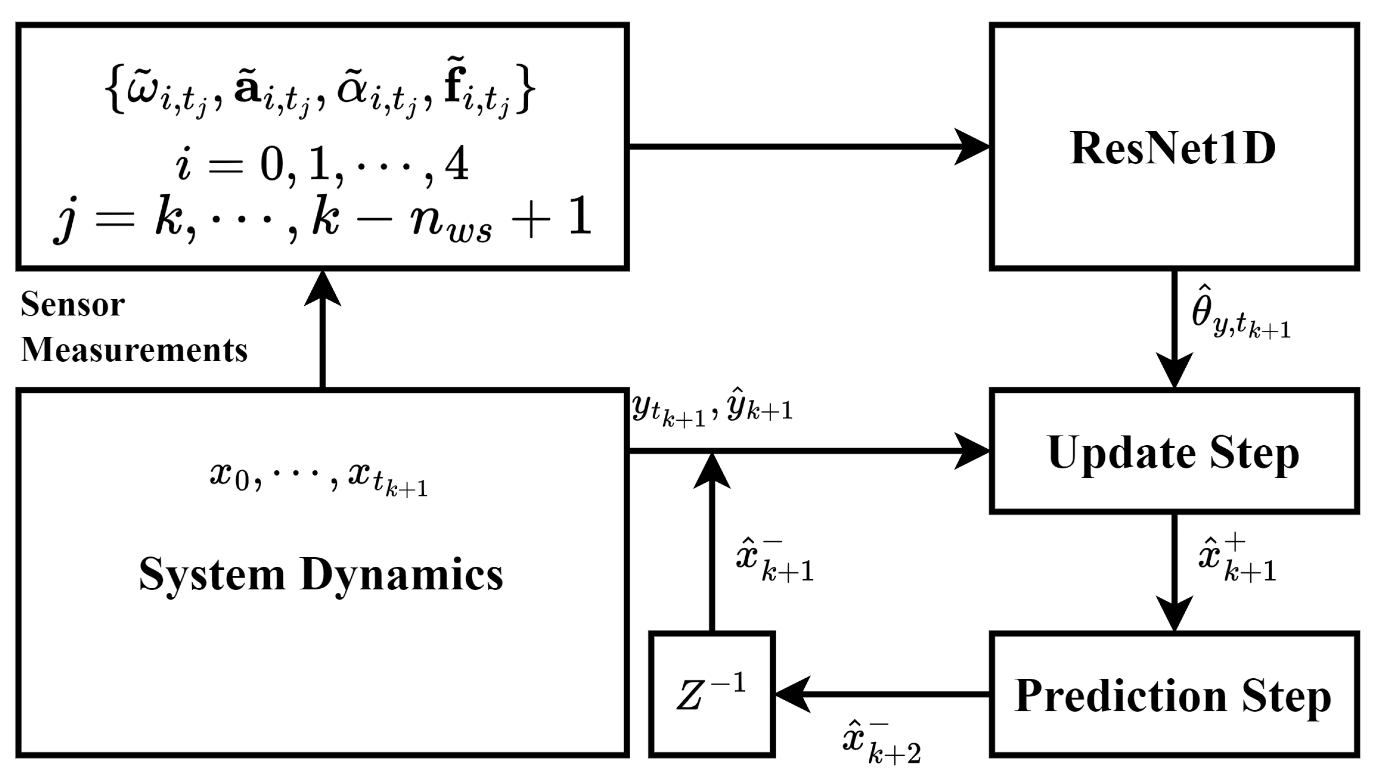
Figure 2.
Comparison of yaw predictions.
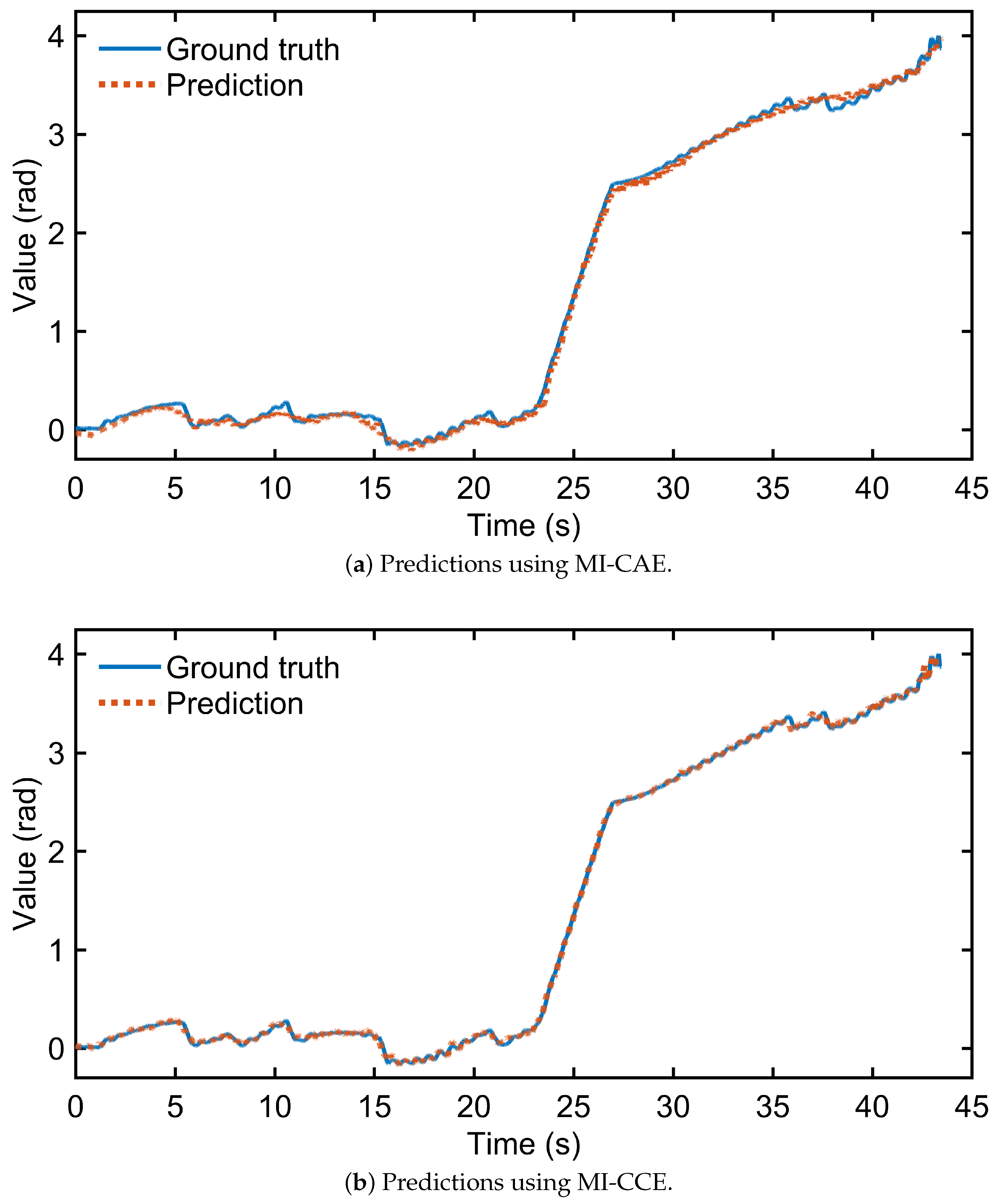
Figure 3.
Trajectory estimation using MI-CCE.
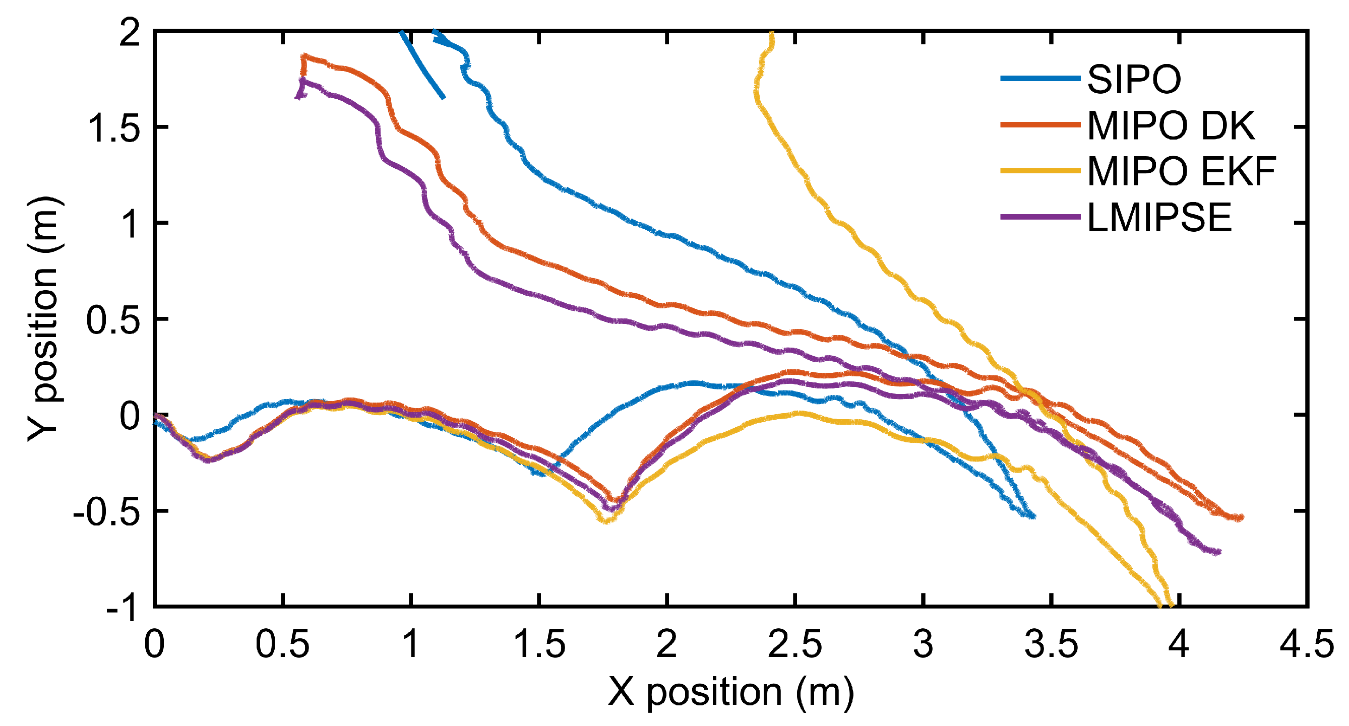
Figure 4.
Comparison of state estimation results.
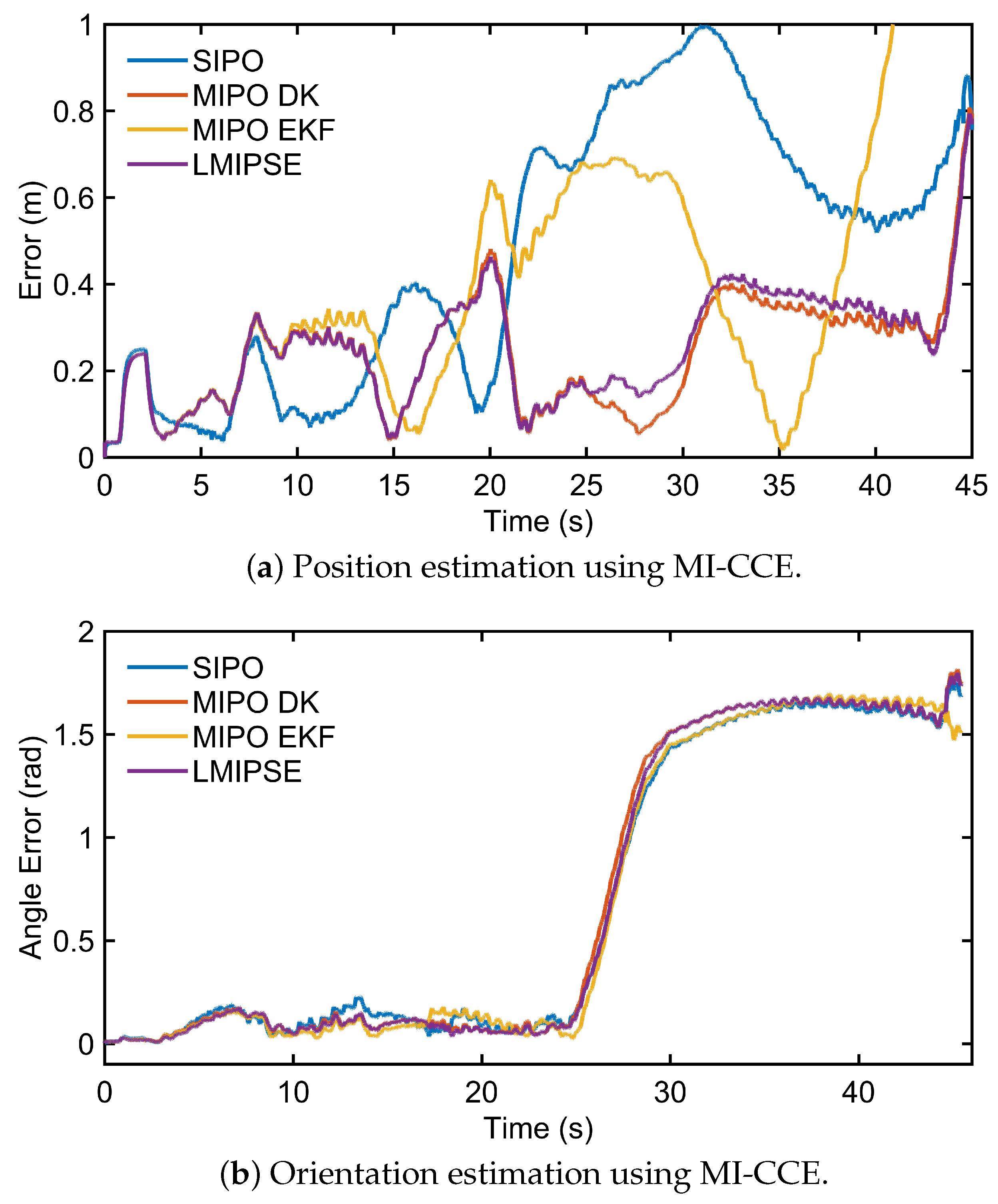

Table 1.
Architecture of the ResNet1D model.
| Layer (type) | Output Shape | Param # |
|---|---|---|
| Conv1d-1 | [32, 256, 8691] | 75,776 |
| MyConv1dPadSame-2 | [32, 256, 8691] | 0 |
| BatchNorm1d-3 | [32, 256, 8691] | 512 |
| ReLU-4 | [32, 256, 8691] | 0 |
| Conv1d-5 | [32, 256, 8691] | 327,936 |
| MyConv1dPadSame-6 | [32, 256, 8691] | 0 |
| BatchNorm1d-7 | [32, 256, 8691] | 512 |
| ReLU-8 | [32, 256, 8691] | 0 |
| Dropout-9 | [32, 256, 8691] | 0 |
| Conv1d-10 | [32, 256, 8691] | 327,936 |
| MyConv1dPadSame-11 | [32, 256, 8691] | 0 |
| BasicBlock-12 | [32, 256, 8691] | 0 |
| ... | ... | ... |
| Conv1d-106 | [32, 1024, 544] | 5,243,904 |
| MyConv1dPadSame-107 | [32, 1024, 544] | 0 |
| BasicBlock-108 | [32, 1024, 544] | 0 |
| BatchNorm1d-109 | [32, 1024, 544] | 2,048 |
| ReLU-110 | [32, 1024, 544] | 0 |
| Linear-111 | [32, 1] | 1,025 |
Table 2.
Testing accuracy of CNN models for different training set sizes.
| Size | 1k | 2k | 3k | 4k | |
|---|---|---|---|---|---|
| Method | |||||
| MI-CAE | 0.0826 | 0.0526 | 0.0464 | 0.0361 | |
| MI-CCE | 0.0445 | 0.0332 | 0.0239 | 0.0236 | |
Table 3.
Summary of results for various state estimation methods under low IMU noise.
| Method | Yaw | Filter | median drift % | RMSE | max RSE |
|---|---|---|---|---|---|
| SIPO | Mocap | EKF | 31.52 | 0.57 | 1.00 |
| SIPO | EKF | EKF | 45.19 | 0.95 | 2.12 |
| MIPO | Mocap | EKF | 14.89 | 0.29 | 0.79 |
| MIPO | DK | EKF | 15.12 | 0.28 | 0.81 |
| MIPO | EKF | EKF | 17.83 | 0.62 | 2.11 |
| MIPSE | RI-EKF | RI-EKF | 16.59 | 0.41 | 1.29 |
| LMIPSE | CAE | EKF | 15.23 | 0.30 | 0.87 |
| LMIPSE | CCE | EKF | 14.84 | 0.29 | 0.80 |
Table 4.
Summary of results for various state estimation methods under high IMU noise.
| Method | Yaw | Filter | median drift % | RMSE | max RSE |
|---|---|---|---|---|---|
| SIPO | EKF | EKF | 45.90 | 0.96 | 2.13 |
| MIPO | EKF | EKF | 18.30 | 0.66 | 2.22 |
| MIPO | DK | EKF | 15.37 | 0.31 | 0.98 |
| LMIPSE | CCE | EKF | 14.87 | 0.29 | 0.79 |
Disclaimer/Publisher’s Note: The statements, opinions and data contained in all publications are solely those of the individual author(s) and contributor(s) and not of MDPI and/or the editor(s). MDPI and/or the editor(s) disclaim responsibility for any injury to people or property resulting from any ideas, methods, instructions or products referred to in the content. |
© 2025 by the authors. Licensee MDPI, Basel, Switzerland. This article is an open access article distributed under the terms and conditions of the Creative Commons Attribution (CC BY) license (http://creativecommons.org/licenses/by/4.0/).
Copyright: This open access article is published under a Creative Commons CC BY 4.0 license, which permit the free download, distribution, and reuse, provided that the author and preprint are cited in any reuse.


