
Submitted:
20 April 2025
Posted:
21 April 2025
You are already at the latest version
Abstract
Point cloud data provides three-dimensional (3D) information about objects in the real world, containing rich semantic features. Therefore, the task of semantic segmentation of point clouds has been widely applied in fields such as robotics, military and autonomous driving. Although existing research has made unprecedented progress, achieving real-time semantic segmentation of point clouds on airborne devices still faces challenges due to excessive computational and memory requirements. To address this issue, we propose a novel sequence convolution semantic segmentation architecture that integrates Convolutional Neural Networks (CNN) with a sequence-to-sequence (seq2seq) structure, termed SeqConv-Net. This architecture views point cloud semantic segmentation as a sequence generation task. Based on our unique perspective of spatially ordered sequences, we use Recurrent Neural Networks (RNN) to encode elevation information, then input the structured hidden states into a CNN for planar feature extraction. The results are combined with the RNN's encoded outputs via residual connections and are fed into a decoder for sequence prediction in a seq2seq manner. Experiments show that the SeqConv-Net architecture achieves 75.5% mean Intersection Over Union (mIOU) accuracy on the DALES dataset, with the total processing speed from data preprocessing to prediction being several times to tens of times faster than existing methods. Additionally, SeqConv-Net can balance accuracy and speed by adjusting hyperparameters and using different RNNs and CNNs, providing a new solution for real-time point cloud semantic segmentation in airborne environments.
Keywords:
seq2seq
; Point cloud
; semantic segmentation
; Recurrent Neural Networks
; Convolutional Neural Networks
1. Introduction
Light Detection and Ranging (LiDAR) devices can directly generate three-dimensional (3D) coordinate information of spatial points, known as point clouds. Due to the accurate representation of 3D shapes of objects, point cloud semantic segmentation is widely used in environmental perception and terrain analysis in remote sensing and mapping. In recent years, with the rapid development of deep learning, research on processing 3D remote sensing data has also achieved unprecedented breakthroughs. Airborne point clouds, as an important category of 3D remote sensing data, can capture more comprehensive and richer information compared to ground-based point clouds, thanks to the high-altitude advantage of drones.
Given the importance and widespread application of point cloud semantic segmentation, many studies have attempted to approach point cloud data from different perspectives for segmentation. The technology of point cloud semantic segmentation has gone through several developmental stages. Traditional methods include Support Vector Machines [1] and Random Forests [2]. Later, researchers proposed methods based on Multi-Layer Perceptrons (MLP) [3], graph-based methods [4], point convolution methods [5], and transformer-based methods [6]. MLP-based methods apply point-wise MLP operations to point clouds and use algorithms like k-nearest neighbors (KNN) for information fusion between points. Graph-based methods model points as graph structures for learning. Point convolution methods, inspired by image convolution, apply 3D point convolution for information extraction and fusion. Recently, due to the success of transformers in natural language processing (NLP) tasks, their structure has also been applied to point cloud semantic segmentation, achieving good results.
1.1. Related Work
1.1.1. Traditional Segmentation Methods
Traditional point cloud segmentation techniques include multi-scale analysis, region growing, clustering, graph cuts, model fitting, and supervoxel methods. Multi-scale analysis methods analyze point cloud features at different resolutions to achieve finer segmentation. Pauly et al. [7] proposed a multi-scale analysis method for point cloud segmentation by analyzing geometric features at different scales. Region growing algorithms start from seed points and merge neighboring points based on local geometric features (e.g., normal vectors and curvature), suitable for planar region segmentation. T. Rabbani et al. [8] proposed a region growing algorithm with smoothness constraints for segmenting planar regions in point clouds. Clustering methods (e.g., K-means and DBSCAN) divide point clouds into clusters for segmentation, with DBSCAN being widely used due to its robustness to noisy data. Graph cut methods build adjacency graphs of point clouds and use minimum cut algorithms to divide the graph into subgraphs, suitable for complex scene segmentation. Golovinskiy et al. [9] proposed a graph cut-based point cloud segmentation method. Model fitting methods extract target structures from noisy data by fitting geometric models (e.g., planes and cylinders). Schnabel et al. [10] proposed a RANSAC-based point cloud segmentation method for extracting geometric shapes like planes and cylinders. Additionally, supervoxel methods divide point clouds into small regions with similar properties, combining geometric and color information for segmentation, providing an effective means for complex scene processing. Papon et al. [11] proposed a supervoxel-based point cloud segmentation method.
After machine learning gained traction, methods relying on manually designed features and traditional machine learning became mainstream. These methods extract geometric features, shape descriptors, or histogram features from point clouds to build classifiers for segmentation. Specifically, geometric features include point cloud structure, normal vectors, and local geometric properties, allowing objects to be modeled as point, line, or surface structures. Rusu et al. [12] proposed a point cloud segmentation method based on geometric features. They computed surface normals, curvature, and point density to build feature vectors and used Support Vector Machines (SVM) for classification, achieving good results in indoor scene segmentation. Shape descriptors model point clouds based on local structural features. Guo et al. [13] proposed a point cloud segmentation method using "Spin Image" shape descriptors to capture local shape information, combined with Random Forest classifiers, showing excellent performance in 3D object recognition and scene segmentation. Histogram features are also widely used. Lai et al. [14] proposed a point cloud segmentation method based on histogram features, using histograms of local geometric properties (e.g., normal direction and curvature) to train classifiers, performing well in outdoor scene segmentation.
1.1.2. Deep Learning-Based Methods
The rapid development of deep learning has significantly advanced point cloud semantic segmenta-tion. In recent years, many excellent point cloud segmentation methods have emerged, which can be broadly categorized into the following types.
Point-based methods: These networks treat point clouds as unordered point sets and directly apply computations to the points without preprocessing, resulting in higher accuracy. PointNet aggregates glob-al features through max pooling, while PointNet++ [15] uses farthest point sampling for downsampling. RandLA-Net [16] introduces random sampling for layer-wise downsampling, and DLA-Net [17] uses learnable attention modules to focus on local features of each point and its neighborhood. Point convolution networks like KPConv and PointConv [18] apply convolution operations directly on points for learning, making them a current research focus.
Projection and multi-view methods: In these networks, researchers project 3D point clouds onto one or more two dimensional (2D) images using specific projection methods, then process the projected 2D images with CNNs to obtain results. SqueezeSeg [19] projects point clouds onto a spherical surface and inputs them into a CNN, while RangeNet++ [20] uses range images as inter-mediate representations. Multi-View CNN [21] projects point clouds from multiple views and concatenates them for segmentation. T
Voxel-based methods: These networks convert point clouds into fixed-resolution grids based on dis-tance or point count and apply 3D convolution or other operations. During voxelization, PointGrid [22] ensures a constant number of points per voxel to retain point cloud density features. VV-Net [23] subdivides each voxel into sub-voxels and uses smooth radial basis functions to re-construct density. SSCNs [24] introduce a convolution operation to alleviate the sparsity issue in voxelization.
Other methods: Other approaches include hybrid segmentation networks, graph-based networks, and transformer-based methods. Hybrid segmentation networks combine the advantages of point and voxel methods. Point-Voxel CNN [25] uses points to capture high-resolution geometric features and voxel convolution to extract low-resolution features. Fusion Net [26] uses point-voxel interaction MLPs to aggregate features. Graph-based networks use Graph Convolutional Neural Networks (GCNs) for processing, but GCNs are complex and are still in the research phase. Recently, transform-er-based networks [27,28,29] have presented a new direction. With their excellent long-range feature capture capabilities, often perform better in point cloud semantic segmentation tasks. Self-attention mechanisms can capture global dependencies in point clouds and com-bines local feature extraction modules to achieve semantic segmentation, showing good performance on multiple datasets.
1.2. Motivations
Due to the inherent characteristics of point cloud data, most of the methods often model point clouds as unordered structures and require time-consuming computations. Some models also need extensive preprocessing before processing can begin. Existing methods often fail to meet real-time requirements on low-power and low-computational devices like drones. Reducing dimensionality and effectively extracting spatial information from point clouds with millions or even billions of points remains a challenge, especially on devices with strict computational and memory resource constraints. This paper aims to develop an efficient point cloud semantic segmentation architecture, SeqConv-Net, to achieve real-time point cloud processing on resource-constrained airborne.
1.3. Contributions
SeqConv-Net is the first method to model voxelated point clouds from the perspective of spatially ordered sequences, using RNNs to encode elevation information into hidden states, which are then input into a CNN for planar spatial feature extraction. Finally, both are fed into a decoder to predict the category of each point. SeqConv-Net is not only compact and fast, but also modular. Any part of it can be combined with mature NLP and image segmentation techniques, and by replacing different RNN encoders/decoders and CNNs, it can balance computational and memory requirements for different tasks allowing customization for specific applications.
In experiments, We designed the first point cloud semantic segmentation network based on the SeqConv-Net framework, with a 2-layer Gated Recurrent Unit (GRU) as the encoder and decoder, and a UNet as the CNN. Experiments show that our network can complete inference in just a few seconds for point clouds with tens of millions of points, even on resource-constrained devices. For point clouds with millions of points, it can perform real-time inference while maintaining good segmentation accuracy. The SeqConv-Net architecture, designed from the perspective of spatially ordered sequences, provides a new approach to point cloud data processing and semantic segmentation tasks. In summary, the contributions of this paper are as follows:
- (1).
- Spatially Ordered Sequence Perspective: We innovatively propose the idea of spatially ordered sequences, where different elevation points at the same planar position can be viewed as a sequence from low to high, with the sequence values containing elevation information. This operates point cloud semantic segmentation as a sequence generation task of the same length, providing a new way to process point cloud data.
- (2).
- SeqConv-Net Point Cloud Semantic Segmentation Architecture: Based on the spatially ordered sequence perspective, we design an RNN+CNN point cloud semantic segmentation architecture called SeqConv-Net, and innovatively use RNN hidden states as CNN inputs to fuse planar spatial information.
- (3).
- Construction and Validation of SeqConv-Net: We design the first network based on the SeqConv-Net architecture and validate its feasibility. Experiments show that our SeqConv-Net design is not only efficient and reliable but also interpretable. Compared to previous methods, it significantly improves the speed of point cloud semantic segmentation in large scenes while maintaining accuracy.
2. Point Cloud Semantic Segmentation Framework
2.1. Architecture Overview
To better balance the trade-off between segmentation accuracy and speed, aiming for efficient real-time segmentation on airborne devices, we propose the SeqConv-Net architecture. This architecture models point clouds from the unique perspective of spatially ordered sequences, treating point cloud segmentation as a sequence-to-sequence generation task. This allows our model to achieve significant speed improvements while maintaining high accuracy compared to existing methods.
As shown in Figure 1, the overall framework is illustrated. Given a range of point clouds, they are first spatially serialized, then an RNN is used to encode elevation information, extracting valid information and mapping it to structured hidden states. The CNN takes this hidden state matrix as input, further fusing information between sequences. Both networks work together to extract information from the XY plane and Z elevation directions, with residual connections. Finally, the decoder generates predictions for each position in sequence.
2.2. Spatially Ordered Sequences
2.2.1. Spatially Ordered Sequences
In the field of point cloud processing, voxelization methods typically down sample point clouds at a fixed spatial resolution, converting them into regular 3D voxel grids. Although this method can transform unstructured point cloud data into a structured representation for 3D convolution operations, its limitations are evident. First, the voxelization process inevitably introduces a large number of empty values (voxels not containing point clouds), which not only fail to provide effective geometric information but also cause a large number of invalid inputs and redundant computations during CNN training and inference. Second, since 3D convolution operations are computationally expensive, the model's efficiency is further reduced.
However, the advantages of voxelization are also significant. It provides an efficient and structured way to process data. By down sampling point clouds in a regularized manner, it reduces data volume while retaining key geometric features of the point cloud, which is particularly important for processing large-scale point cloud data. Additionally, voxelization converts point clouds into regular 3D grids, where the absolute and relative positions of each voxel in space are explicit and fixed. This inherent regularity eliminates the need for additional KNN algorithms to extract spatial relationships between points, simplifying the feature extraction process. Moreover, the structured point cloud after voxelization can be processed using more mature convolution algorithms, making it highly compatible with existing deep learning frameworks and facilitating efficient parallel computing.
To address the issue of empty values in traditional voxelization methods while leveraging the advantages of voxelization in down sampling and structured representation, we propose a novel perspective on point cloud voxel representation—spatially ordered sequences. This idea is inspired by the way humans perceive 3D space: when observing a 3D scene, if there are gaps between objects in the elevation direction, the brain typically ignores these gaps and naturally expresses the effective points in space as a sequence from low to high. This cognitive approach provides important insights: during voxelization, invalid voxels caused by gaps between objects at different elevations do not need to be explicitly stored or processed. Instead, only the valid voxels are organized into sequences of varying lengths to effectively represent vertical spatial changes.
Specifically, let vector:
represent the voxel distribution along the vertical direction at a planar position after voxelization (note that the values here are in bold black to indicate the difference from the numbers), where represents the-th valid voxel from bottom to top, and represents invalid voxels caused by spatial discontinuities. The generated spatial sequence is:
where is a special voxel artificially added after the last valid voxel in each spatial sequence, marking the end of valid voxels (the fast generation algorithm for spatial sequences is detailed in the next section).
Spatially ordered sequences arrange valid voxels at each planar position in elevation order, forming a dynamically sized sequence. This approach effectively down samples point clouds while retaining spatial structural information, improving data compactness and computational efficiency. During serialization, all valid positions are pushed to the front, allowing the RNN to avoid processing intermediate padding positions. The special end voxel also ensures that the RNN correctly learns the valid parts of the sequence, excluding the influence of padding voxels at the end.
In traditional voxelization, the average elevation of points in a voxel is often used to represent the voxel's position. However, to enable the use of embedding techniques from NLP tasks, the elevation representation in spatially ordered sequences is entirely different. Specifically, we use the voxel's index as the elevation representation in the spatially ordered sequence. For the spatially ordered sequence ,the elevation representation using voxel indices is:
where is used as a padding value to fill the sequence to the required length, and each number represents the index of the valid voxel in the original plus one. Figure 2 also illustrates the serialization process for a voxel matrix of shape (4,3,4) (following the deep learning convention, matrix rows and columns are at the back).
This index-based elevation representation has four significant advantages:
- (1).
- Avoids issues with absolute elevation: Traditional methods using elevation coordinates may face inconsistencies or computational complexity due to variations in elevation range or noise. Using indices as elevation representations converts elevation information into relative positional relationships, avoiding instability caused by absolute elevation values and enhancing model robustness.
- (2).
- Fast generation of spatially related sequences: The index-based elevation representation allows for accelerated sequence generation using sorting algorithms. By sorting the sequence and using the indices of valid positions as input, spatial sequences can be quickly generated. This serialized representation facilitates efficient computer processing and significantly reduces preprocessing time compared to methods like KNN, especially for large-scale point cloud data.
- (3).
- Utilizes NLP embedding methods: By using integer indices as elevation representations, we can leverage embedding techniques from NLP, mapping indices to high-dimensional vector spaces for computation. This embedding representation captures relationships between elevations and provides richer feature representations for deep learning models, enhancing their expressive power.
- (4).
- Efficient voxel-to-point cloud recovery: During prediction, the network can sequentially output predictions for each valid position and use the indices to restore the correspondence between predictions and original voxels. This recovery process is computationally efficient and does not introduce additional losses.
2.2.2. Generation Algorithm for Spatially Ordered Sequences
Spatially ordered sequences not only facilitate RNN encoding but also have a simple and fast generation algorithm.
Let vector:
represent the voxel distribution at a planar positionafter voxelization. By setting valid positions to 1, a mask vector:
is generated. Adding an end marker at the end of the mask vector results in the padded mask vector:
To push valid positions to the front, we use an order-preserving sorting algorithm to sort obtaining the sorted result and the corresponding indices:
where:
The generated spatial sequence is:
The purpose of +1 is to leave index 0 as the padding position.
With the spatially ordered sequence, a corresponding label sequence is needed for training. For the label sequence, let vector:
Similarly, a 0 is appended at the end to match the length of .Thus:
where is the mode of the labels of all points in the th valid voxel.
To generate the sequence-form label and the teacher-forcing input ,the sorting indices Index from the spatially ordered sequence generation process is used:
Using sorting algorithms, the generation of spatially ordered sequences can be accelerated with hardware-friendly operations, leveraging sorting algorithms with a time complexity of .
2.2.3. Differences Between Spatially Ordered Sequences and NLP Sequences
Although voxelated point clouds share similarities with sequences in NLP, there are significant differences due to the inherent characteristics of point cloud data.
First, in NLP, tokens can appear multiple times at different positions, and each token has its semantic meaning, making NLP sequence processing more flexible and diverse. However, in spatially ordered sequences, the values represent elevation information, which follows a strict order. This strict ordering leads to sequences that are strictly increasing in elevation, making them strictly ordered. This strictness plays an important role. It simplifies the model's learning task, as the model does not need to handle complex contextual repetitions or long-range dependencies as in NLP. The strict ordering also makes the generation and processing of spatial sequences more efficient. In sorting and indexing operations, the elevation order allows for rapid sequence generation.
Second, in NLP, the effective length of sequences is usually long, and in some large-scale tasks, the sequence length can reach thousands or even tens of thousands. This long-sequence characteristic requires NLP models to have strong context capture and long-range dependency modeling capabilities. In contrast, in real-world scenarios, the effective length of point cloud sequences at the same planar position is usually short, typically not exceeding a few dozen to a few hundred. This short-sequence characteristic makes the learning task for point cloud sequence data relatively simpler, allowing the model to more easily learn elevation and spatial distribution patterns while reducing computational complexity.
2.3. Spatial Information Processing
2.3.1. Elevation Information Extraction Using RNNs
Point cloud data differs fundamentally from common 2D image data, as it not only contains 2D planar coordinate information, but also elevation information. This 3D characteristic makes point cloud data richer and more complex in expressing spatial structures while also posing significant challenges for data processing. How to effectively process and fuse information from these three dimensions is a core issue in point cloud data processing. Current popular methods rely on KNN, 3D CNNs, projection, point convolution, transformers, etc., which attempt to simultaneously extract and fuse 3D information. However, these methods often struggle to balance computational efficiency and feature extraction accuracy.
To address this issue, we adopt a divide-and-conquer strategy for 3D information: first, we fuse features in the elevation direction, and then we fuse the already fused features in the planar direction. This divide-and-conquer strategy not only reduces computational complexity but also better captures unique information in each dimension.
Recurrent Neural Networks [30], with their unique structural design, have shown significant advantages in processing variable-length sequence data. Through their recurrent mechanism, RNNs can process each element in the sequence step by step, passing information from previous steps to the current step, effectively capturing contextual information in the sequence.
In natural language processing, RNNs have been proven successful in various tasks such as language modeling, machine translation and text generation. In these tasks, text sequences of different lengths are mapped to fixed-length hidden states after being processed by RNNs. These hidden states not only represent local features of the sequence but also capture global contextual information, comprehensively characterizing the semantic and structural features of the entire sequence.
In NLP, for an input at time step with batch size and embedding dimension , the RNN encoder updates the current hidden state as follows:
where is the current hidden state, is the previous hidden state, is the output at the current time step, and and are the weights and biases of the output layer. This means that RNNs have the ability to integrate sequence information, and the final hidden state will possess the ability to characterize the entire sequence.
Inspired by the successful application of RNNs in NLP tasks, we can model and process point clouds from the perspective of spatially ordered sequences. By embedding each valid position's elevation index into a dense vector representation and sequentially inputting these embedded vectors into the RNN, the recurrent structure can process each valid voxel's position information step by step, passing feature information from previous positions to subsequent processing steps. Finally, the RNN outputs a fixed-length hidden state that captures both local geometric features of each valid position in the sequence and the global spatial structure information of the entire sequence (Figure 3). In this way, unstructured spatially ordered sequences can be encoded into structured hidden states for further processing.
2.3.2. Planar Information Fusion and Extraction Using CNNs
While RNNs encode hidden states, they only consider the sequential relationships between valid voxels in the elevation dimension and ignore the spatial relationships between adjacent voxels in the same planar space. In other words, RNNs can only fuse and extract information from valid voxels along the elevation dimension (i.e., the sequence direction) and map this information into a fixed-length hidden state. Although this hidden state can characterize local and global features of valid voxels in the elevation direction, it completely ignores the distribution information of point clouds in the planar direction.
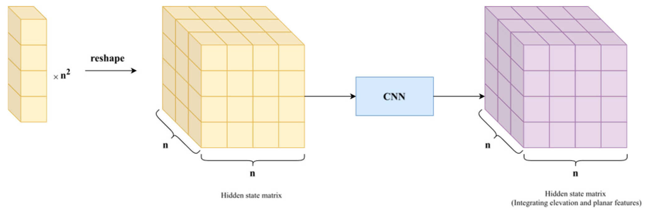
Therefore, to more comprehensively extract the spatial structural features of point cloud data, it is necessary to further extract and fuse planar position information. In the extraction and fusion of planar position information, CNNs [31] have been widely used and proven to be one of the best solutions. Through their local receptive fields and weight-sharing mechanisms, CNNs can efficiently capture local patterns in 2D space, making them highly effective in image semantic segmentation and classification tasks. Based on this mature technology, we can combine the elevation information extracted by RNNs with the planar information extracted by CNNs to achieve 3D feature fusion of point cloud data.
To enable CNNs to process these hidden states, the hidden variables can be arranged according to their original planar positions to form a hidden variable matrix. Each element in this matrix is a hidden state vector generated by the RNN from that position. Through this operation, the planar spatial structure is restored while retaining elevation information.
Figure 4.
Planar information extraction using CNNs.
After the CNN processes the hidden variable matrix, the simplest approach is to feed the output directly into the RNN decoder. However, this can be improved. CNNs often use downsampling layers to reduce feature map resolution, lowering computational complexity and expanding the receptive field. Yet, this operation sacrifices fine-grained details, which are critical for small objects or complex structures in point clouds.
Instead of directly feeding the output to the RNN decoder, we propose a better strategy: connecting the CNN's output with the initial hidden variables via a residual structure [32] before inputting them into the decoder.
RNNs often face steep loss function spaces, leading to vanishing or exploding gradients during backpropagation. The residual structure provides a more direct gradient flow from the decoder to the encoder.
Moreover, the initial hidden variables, generated without downsampling, retain rich detail information from the elevation direction. By combining the CNN's output with these initial hidden variables through a residual connection, the model compensates for detail loss during downsampling, enhancing its ability to reconstruct small objects and complex structures.
2.3.3. Prediction
In seq2seq [33] models, the prediction process is typically performed recursively (Fig. 5), where the model uses the previous output as the next input, combined with the hidden state, to generate the output sequence step by step until the model predicts the end token. This mechanism is common in tasks such as machine translation and text generation, where the output sequence length is usually variable, and the model needs to dynamically decide when to stop generating.
In our SeqConv-Net structure, the prediction process differs from traditional seq2seq models due to the nature of semantic segmentation tasks. In semantic segmentation tasks, there is a strict correspondence between input and output: each valid voxel must be assigned a corresponding prediction label, while invalid voxels should not participate in the prediction. In other words, semantic segmentation tasks require that the effective lengths of the input and output sequences at each spatial position must be exactly the same. This strict constraint leads to some differences between the SeqConv structure and seq2seq models during training and prediction.
Seq2seq models need to learn how to dynamically determine the length of the output sequence particularly when to generate the end token to terminate the prediction process. In the SeqConv structure, since the effective lengths of the input and output are fixed, the model does not need to learn how to predict the end token but only needs to focus on accurately predicting the first part of the effective length. Specifically, during training, the SeqConv-Net structure does not need to include the end token as part of the output, and during prediction, the model does not need to concern itself with whether the sequence should end. The model must predict a specified number of times, and predictions beyond that number should be invalid. Figure 5 illustrates the prediction process of the SeqConv structure, where the RNN decoder is initialized with the hidden state output by the encoder and the Start token to generate the first prediction. Subsequently, the previous prediction and the updated hidden state are used for the next prediction until the prediction length matches the effective length of the input sequence.
where:
The fixed-length to fixed-length sequence mapping characteristic of semantic segmentation tasks makes the SeqConv structure more efficient and straightforward in semantic segmentation tasks. It avoids the complexity and uncertainty introduced by dynamic length prediction and makes batch prediction more convenient.
During batch prediction, the model can generate corresponding prediction vectors by specifying a sufficient number of prediction steps. However, since the effective lengths of input sequences vary, the model needs to use the maximum length as the prediction length during batch prediction. Therefore, for sequences with shorter effective lengths, the model will generate results beyond the actual effective length. To filter out irrelevant prediction results, we can use the one-to-one correspondence between input and prediction in semantic segmentation tasks. Assuming the prediction sequence at a planar position is:
Using the sorted mask vector:
from the spatial sequence generation process, multiplying the two yields the prediction results only for valid positions. Additionally, to maintain length consistency, a is appended at the end:
However, although masking can remove irrelevant prediction values, the prediction vector still cannot directly correspond to each point in the original point cloud. This is because, during serialization, all valid voxels are pushed to the front of the sequence, so the prediction results cannot correctly correspond to the original voxels. However, since elevation is represented using indices, we can use the sorting indices obtained during serialization to perform an inverse operation for recovery.
For the sorting indices:
obtained during sequence generation; in order to use these indices for deserialization, we need to sort them again:
where:
The deserialization operation is then:
Discarding the 0 at the end used for padding, we obtain the true prediction vector:
Comparing this with the original voxel vector:
We can see that we have restored the correspondence between the category values in the prediction vector and the original voxels. Then, using the coordinates of points in the voxel matrix, we can obtain the correspondence between each point and its predicted value.
3. Experimental Results and Analysis
3.1. Data Preprocessing and Augmentation
3.1.1. Sequence Loss
Spatial serialization is the foundation of the SeqConv-Net structure, and its approach is a crucial factor in determining the model's capabilities. The results of serialization at different resolutions may have a significant impact on the final convergence. Since the label of each voxel during serialization is determined by the mode of the labels of the points within it, deserialization inevitably cannot precisely restore the category of each point. However, the extent of this loss needs to be quantified. Given the limited availability of large-scale airborne point cloud datasets, many datasets only contain a few million points, making them less valuable for reference. Therefore, we selected the DALES dataset as our benchmark dataset.
DALES: A Large-scale Aerial LiDAR Data Set for Semantic Segmentation [34]. This is a new large-scale aerial LiDAR dataset with over 500 million manually labeled points, covering an area of ten square kilometers and eight object categories. DALES is the most extensive publicly available ALS, with 400 times more points than other currently available annotated aerial point cloud datasets and six times the resolution.
Additionally, the dataset suffers from severe class imbalance. The three classes ground, vegetation and buildings account for 98.1% of the training set points, making this dataset highly challenging, not only due to its large scale but also because it measures the model's ability to learn from small samples.
To quantitatively measure the loss caused by serialization, we performed serialization on the DALES dataset at three common resolutions and obtained corresponding labels. We then used these labels to deserialize and restore the category of each point, comparing them with the true categories. The results are shown in Table 1 and Figure 6.
From the table, it can be observed that the deserialization loss is closely related to the actual shape and position of the objects. Among
From the table, it can be observed that the deserialization loss is closely related to the actual shape and position of the objects. Among small objects, power lines and fences, both linear objects show significant differences in deserialization loss. At a one meter resolution, the IOU difference between them can reach approximately 0.15. This is because power lines are usually suspended in the air and maintain a relatively independent spatial relationship with surrounding objects, allowing them to be separated during serialization. In contrast, fences, as low ground objects, are often close to ground vegetation and buildings, leading to higher loss during low-resolution serialization.
Among large objects, the IOU difference between buildings and vegetation after deserialization can reach 0.07. This difference is mainly due to the geometric features and spatial distribution patterns of these two classes. Buildings typically have regular geometric shapes (rectangular or regular polygons) and clear boundary features, with relatively independent spatial distributions. Vegetation, on the other hand, often has irregular contours and complex spatial interactions with roads and buildings, leading to some loss during serialization, though the loss is less severe compared to small objects like fences.
- (1).
- From the global accuracy perspective, even at the maximum resolution of one meter, the model's mIOU remains at 0.93. This result indicates:
- (2).
- The impact of serialization on object classification accuracy is within an acceptable range, and higher resolutions lead to greater serialization loss.
- (3).
- The accuracy differences between different object classes are mainly due to their inherent geometric features and spatial distribution characteristics, rather than the serialization process itself.
3.1.2. Elevation Truncation
In the real world, terrain elevation is unbounded, but to meet the input requirements of deep learning models, a reasonable upper threshold must be set for elevation data. This study uses the truncation method to handle data exceeding the preset elevation range. Specifically, for any point exceeding the maximum elevation threshold (i.e., with an index greater than the threshold) after serialization, its elevation value is set to the maximum elevation value. During the prediction phase, the predicted labels for these truncated positions will be assigned to all points above this elevation. By truncating the sequence rather than the point cloud itself, the model can still predict all points even if it cannot input the entire elevation range.
Figure 7 qualitatively demonstrates the effect of the truncation method, all within an actual area of 100 meters * 100 meters. In the first example, some vegetation is truncated due to exceeding the preset 50-meter elevation limit, but these trees are still classified as vegetation from the truncation layer to the canopy. In the second example, a high-rise building is truncated during serialization, but it is still classified as a building from the truncation layer to the top. The effectiveness of this method is based on an important geospatial phenomenon: objects significantly higher than their surroundings usually have vertical continuity
To quantitatively evaluate the impact of truncation, we set a truncation elevation of 50 meters at a 0.5-meter resolution and compared the IOU accuracy with and without truncation in regions where truncation occurred. As shown in Table 2, the truncation operation has no impact on the IOU accuracy of the DALES dataset at the third decimal place. It can be concluded that the truncation method is both effective and efficient for data preprocessing. It not only meets the length requirements for embedding but also has a negligible impact on final classification accuracy
3.2. Experiments
3.2.1. Network Structure
When implementing the model using the SeqConv architecture, we designed the first model based on a balance between efficiency and accuracy, as shown in Figure 9. The RNN encoder and decoder of this model both use 2-layer Gated Recurrent Units [35]. The reason why we choose GRU instead of LSTM [36] is that LSTM often performs better when processing long sequences. However, due to the second characteristic of spatially ordered sequences (they are generally short in length), it is better to use a lighter GRU. For the CNN part, UNet [37] as a classic encoder-decoder structure, is widely used in image segmentation tasks. Its skip connections effectively preserve multi-scale spatial information, so we chose the well-tested UNet structure. This design leverages the lightweight characteristics of both GRU and UNet to maintain low computational complexity while using GRU's gating mechanism to more effectively retain key information in sequences.
Since spatially ordered sequences are usually short, the information contained in their hidden states is not as extensive as in NLP tasks, so the hidden state dimension does not need to be as large as hundreds or thousands. From an efficiency perspective, excessively long hidden state dimensions significantly increase computational burden. In practice, we chose hidden state dimensions between 16 and 48.
3.2.2. Elevation Embedding
Although spatial sequences are similar in form to sentences in NLP tasks (i.e., both are composed of a series of elements), there are fundamental differences in encoding methods. In NLP, pre-trained word vector models such as Word2Vec [38] and GloVe [39] usually map semantically similar words to nearby positions in the vector space to achieve better convergence. However, the values in spatial sequences represent elevation information, not semantic information.
In the encoding of elevation sequences, using NLP word embedding methods directly can lead to serious problems. Word embedding methods assume that similar words have semantic similarity, so they map distant tokens in the vocabulary to nearby vectors. However, elevation values do not have semantic meanings and should not be assumed to have specific relationships. Therefore, if word embedding methods are directly used to encode elevations, the model will fail to capture the physical positional relationships between elevations and instead will force certain elevations to have specific relationships, which leads to severe overfitting.
Fortunately, there are mature solutions for encoding positional information. In transformer models, to utilize positional information in sequences, researchers propose the concept of positional encoding. The following method is used to encode elevations:
For a given input sequence of length , its -dimensional positional encoding [40] is represented as , where the elements at row , column , and column are:
Positional encoding adds absolute or relative positional information to the input representation, allowing the model to perceive the positional relationships of each element in the sequence. This positional encoding method aligns well with the encoding needs of elevation sequences. Positional encoding generates fixed encoding vectors using sine and cosine functions, with frequency changes representing absolute positions. Since positional encoding is fixed, it does not introduce additional trainable parameters and can accelerate the training process.
In experiments, we tried two different elevation encoding methods: trainable random embeddings and fixed cosine encoding. When using trainable random embeddings, the model performed well on the training set but showed severe overfitting on the test set, with the mIOU difference between the training and test sets reaching up to 0.2-0.3. This phenomenon occurs because trainable random embeddings cause the network to attempt to memorize the distribution of elevation values through training data and assign non-existent relationships, completely ignoring the physical positional relationships of elevation values. Therefore, when encountering unseen elevation distributions in the test set, the prediction accuracy drops significantly.
When we changed the encoding method to fixed cosine encoding, the overfitting problem was significantly alleviated, improving the model's accuracy on the test set by up to 0.1-0.2, while also speeding up convergence. The elevation encoding vectors generated by sine and cosine functions effectively represent the physical positional relationships between elevations without introducing additional trainable parameters. This forces the network to avoid memorizing elevation distributions by altering embedding vectors, ultimately preventing overfitting and enabling the model to better capture regular relationships between elevations, improving robustness and convergence speed. This strongly confirms the first characteristic of spatially ordered sequences: the elevation positional nature of spatially ordered sequences requires that embedding vector represents elevation positions rather than semantics.
3.2.3. Implementation Details and Evaluation Metrics
In the experiments, we used the PyTorch framework to implement our network. During data preprocessing, the only required preprocessing step was dividing the dataset into 100 square meters areas. For the training process, after serialization, each block was input as a 160160 matrix. For a 0.5-meter resolution, this means inputting a ground area of 80 square meters at a time. Thanks to the compactness of our network and the advantages of spatial sequences, even with a hidden state dimension of 32, our network only requires a 16GB RTX 4070 Ti for training and a 4GB GPU for inference.
Additionally, we used the Adam optimizer to minimize the objective function, with mIOU as our evaluation metric. The training lasted for 100 epochs, and data augmentation was turned off in the final few epochs. The loss function used a combination of CrossEntropyLoss and DiceLoss, and the UNet network had layers of [64, 128, 256, 512, 1024].
3.2.4. Results on the DALES Dataset
To comprehensively evaluate the performance of various models in practical applications, we specifically tested their running speed on mobile devices with limited computational resources. These devices typically have low computational power and limited memory, placing higher demands on model efficiency. In experiments, we selected a complete 500-square-meter test set containing 12,219,779 points as a benchmark to measure the processing speed of different models under the same mobile hardware environment.
To ensure the test results accurately reflect model performance and exclude pre- and post-processing factors, we adopted stricter statistical standards for fairness. All models were evaluated without accelerated inference or quantization, and the time measured included not only the model's inference time but also all preprocessing steps from reading the raw point cloud data to input. This approach clearly demonstrates the significant speed advantages of the SeqConv-Net structure and its spatially ordered sequence method. Table 3 shows the mIOU metrics and time consumption (in seconds) of various models
From the results, the GRU-UNet network, as the first model implemented with the SeqConv-Net structure, not only maintains segmentation accuracy but also shows a significant improvement in speed compared to other models. This outstanding performance is not only due to the elegant design of the SeqConv-Net structure itself, but is also closely related to its unique input representation method—the generation of spatially ordered sequences.
Figure 10.
Segmentation results of the GRU-UNet network on the DALES dataset.
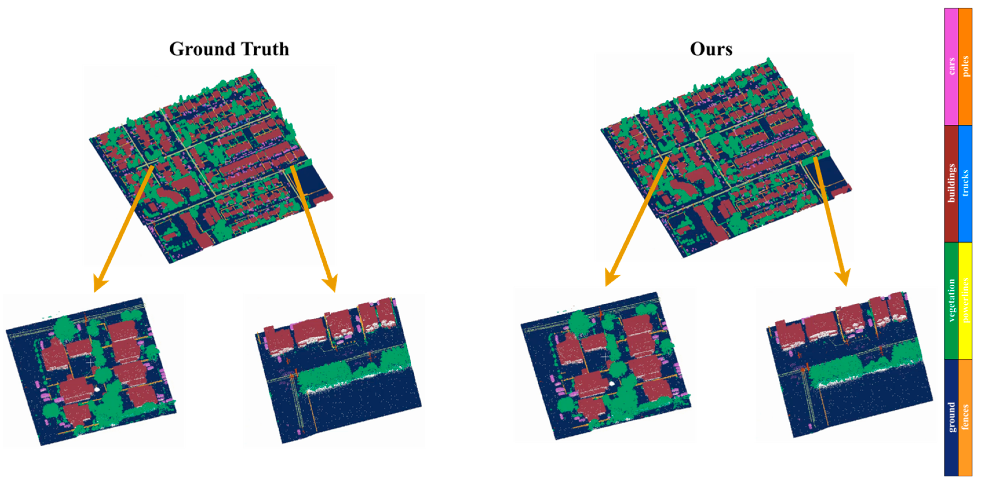
By combining the spatial local perception ability of CNNs and the sequence compression and extraction ability of RNNs, SeqConv-Net achieves extremely fast inference speeds while maintaining high accuracy, thanks to its hardware-friendly characteristics. Additionally, the construction of spatially ordered sequences leverages mature fast sorting algorithms, enabling the rapid transformation of unordered point clouds with tens of millions of points into spatially ordered sequences. Together, these factors contribute to SeqConv-Net's overwhelming speed advantage. Whether for real-time processing of large-scale point cloud data or lightweight deployment in resource-constrained environments, SeqConv-Net demonstrates unparalleled speed.
Although the GRU-UNet, as a network based on the SeqConv-Net architecture, may not yet achieve optimal performance, it is only the simplest model implemented with the SeqConv-Net concept. Therefore, by combining mature NLP techniques and advanced image semantic segmentation techniques with SeqConv-Net, we believe it can we believe it can allow for new possibilities in the field of point cloud processing.
3.3. Ablation Studies
3.3.1. Hidden State Dimension
The dimension of hidden states limits the amount of information the model can retain after encoding, thus having a decisive impact on the model's learning ability. In NLP tasks, embedding lengths and hidden state dimensions are often long, reaching hundreds or even thousands. However, the SeqConv-Net structure does not require such long dimensions. For different hidden state dimensions, we evaluated their final convergence results on the DALES dataset.

Table 4.
IOU of Different Classes for SeqConv-Net with Different Hidden State Dimensions.
| ground | vegetation | buildings | cars | trucks | poles | powerlines | fences | mIOU | speed | |
| 16 | 0.942 | 0.839 | 0.930 | 0.655 | 0.396 | 0.679 | 0.607 | 0.406 | 0.682 | 4.05s |
| 24 | 0.950 | 0.851 | 0.931 | 0.685 | 0.412 | 0.681 | 0.658 | 0.453 | 0.702 | 4.26s |
| 32 | 0.953 | 0.870 | 0.932 | 0.732 | 0.453 | 0.704 | 0.717 | 0.495 | 0.732 | 5.56s |
| 40 | 0.952 | 0.896 | 0.932 | 0.763 | 0.522 | 0.701 | 0.704 | 0.501 | 0.747 | 6.02s |
| 48 | 0.964 | 0.919 | 0.934 | 0.751 | 0.532 | 0.706 | 0.724 | 0.511 | 0.755 | 8.01s |
Figure 11.
Segmentation results with different hidden state dimensions. As the hidden state dimension increases, the segmentation effect for small objects gradually improves.
Figure 11.
Segmentation results with different hidden state dimensions. As the hidden state dimension increases, the segmentation effect for small objects gradually improves.
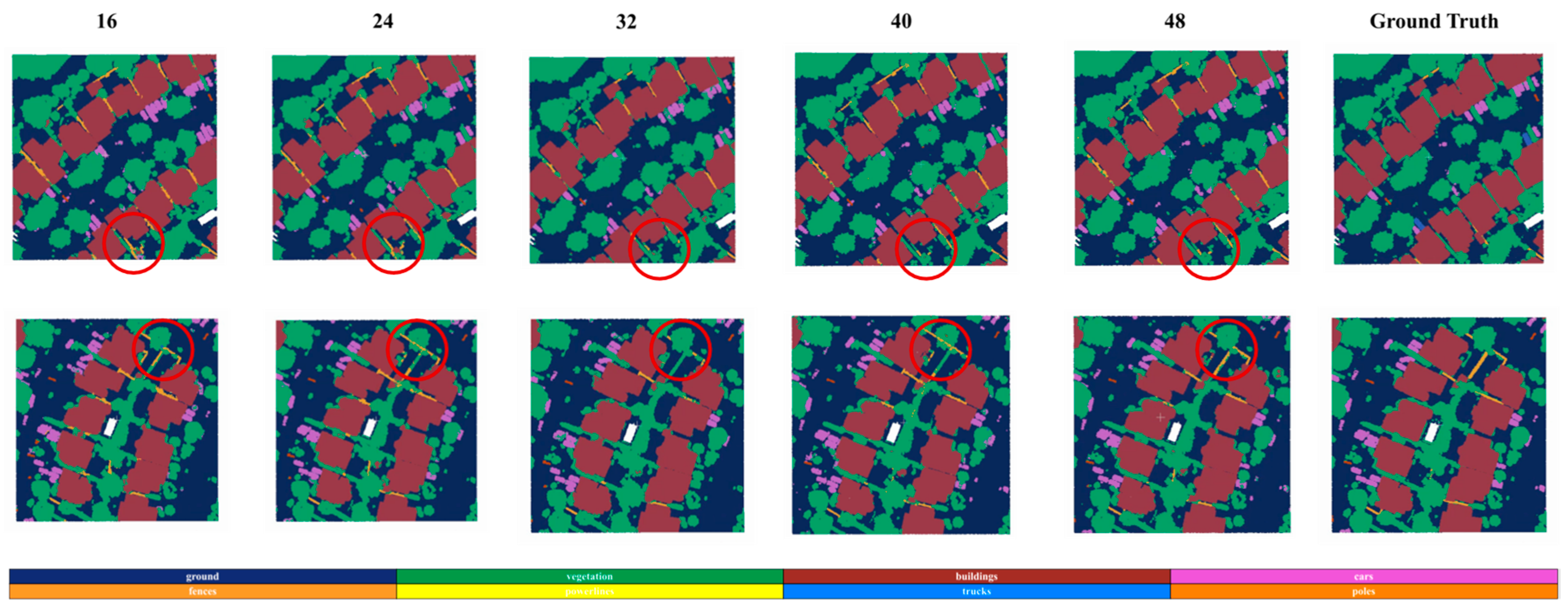
It is clear that as the hidden state dimension increases, the model's final convergence accuracy also improves. However, as the dimension continues to grow, the improvement in accuracy gradually diminishes and saturates. This phenomenon validates the second important characteristic of spatially ordered sequences: their short length. Since spatially ordered sequences are short and carry relatively limited information, excessively high hidden state dimensions are not necessary for efficient encoding and information retention.
Additionally, by analyzing the performance of different classes at various hidden state dimensions, we observe that for larger and more prominent objects (e.g., ground, buildings, and poles), the improvement in accuracy with increasing hidden state dimension is minimal. In contrast, for small target classes (e.g., cars, trucks, poles, and fences), the improvement in accuracy is significant. This indicates that for difficult-to-classify small targets, appropriately increasing the hidden state dimension can effectively enhance the model's ability to learn fine-grained features, significantly improving segmentation accuracy.
3.3.2. Spatial Sequence Resolution
The spatial resolution used during serialization has a decisive impact on loss. Higher resolutions lead to more severe loss of small targets during serialization. Therefore, we also evaluated model training at three common resolution settings. The hidden state dimension was set to 32, and other hyperparameters remained consistent
Table 5.
IOU of SeqConv-Net with Different Serialization Resolutions.
| ground | vegetation | buildings | cars | trucks | poles | power lines | fences | mIOU | speed | |
| 1 | 0.943 | 0.839 | 0.930 | 0.512 | 0.214 | 0.682 | 0.651 | 0.210 | 0.622 | 1.51s |
| 0.5 | 0.953 | 0.870 | 0.932 | 0.732 | 0.453 | 0.704 | 0.717 | 0.495 | 0.732 | 8.01s |
| 0.25 | 0.955 | 0.865 | 0.925 | 0.713 | 0.421 | 0.692 | 0.653 | 0.512 | 0.717 | 30.9s |
However, higher resolutions did not lead to the expected accuracy improvement. Further analysis shows that at lower resolutions, the sequence length increases significantly, introducing many valid voxels with similar elevations. These elevations, after continuous encoding, often result in significant information redundancy. Additionally, the two-layer GRU's learning ability is limited, making it difficult to filter out more valuable elevation information and leading to reduced model accuracy.
Lower resolutions make small target detection more difficult, reducing accuracy. However, this reduction is not without benefits. When the resolution is halved, the total number of sequences generated decreases to one-fourth, resulting in nearly four times the speed improvement. In practice, this means that if a slight sacrifice in small target accuracy is acceptable, the speed can easily reach tens of millions of points processed per second.
3.3.3. Exploring Hidden Variables
In CNNs, each channel of an image represents a feature channel that characterizes a specific feature. Does the SeqConv-Net structure exhibit similar behavior? The answer is yes. Since the input sequences are arranged by elevation, it can be inferred that these 16 channels should have a significant correlation with the Digital Surface Model (DSM). Therefore, we generated DSM images from the point cloud data and compared them with the visualization results of the 16 channels (Figure 12).
The results show that these channels exhibit visible similarities with the DSM and changes in object categories. In particular, in the 4th channel, ground in the DSM strongly correspond to light-colored regions, indicating that the model successfully identified and distinguished ground points from non-ground points during encoding and embedded this information into these channels. In the 1st and 2nd channels, the response for the fence category, which is close to the ground elevation, is almost zero. This shows that the model not only learned to embed information in individual channels but also learned to decompose and reorganize information across different channels.
These strong correspondences with the DSM demonstrate that the GRU encoder and CNN's processing of hidden variables essentially constitute a "high-dimensional projection" mechanism. This mechanism effectively compresses and reorganizes multi-dimensional information from the original 3D data through specific feature extraction methods, embedding different types of key feature information into different channels of the hidden variables.
Compared to general projection methods, the effectiveness of this high-level abstract information projection mechanism lies in the following aspects:
- (1).
- The focus of different channels on specific object features indicates that the model does not simply encode elevations, but learns spatial information perception through the CNN which enables the model to learn feature separation methods.
- (2).
- The complementary feature distribution across channels shows that the model achieves effective information decomposition and reorganization, not just simple encoding.
- (3).
- The correspondence between features and the DSM confirms that the hidden variable mapping process has practical physical significance.
These findings validate the rationality of the SeqConv-Net structure from both theoretical and practical perspectives. Theoretically, the GRU encoder uses its gating mechanism to filter and memorize elevation information, extracting representative features. The CNN, through its convolutional kernels' spatial perception ability, further captures the spatial correlations of local features. The synergy between the two achieves multi-level, multi-scale feature extraction of 3D data.
Practically, the SeqConv-Net structure can rapidly extract and map information from point clouds, achieving efficient encoding of 3D data. The model's interpretability is strong. By analyzing the feature response patterns of different channels, we can clearly observe how the model transforms raw data into feature representations with physical significance. This transformation process retains the key spatial information of the original data while improving information usability through feature reorganization. Therefore, the design of the SeqConv-Net structure is not only an effective solution for point cloud segmentation but also an innovative exploration of 3D data processing theory.
4. Conclusions
This paper addresses the issues of high computational resource consumption and insufficient real-time performance in large-scale airborne point cloud semantic segmentation tasks by proposing an innovative lightweight architecture: SeqConv-Net. This architecture voxelates point clouds into spatially ordered sequences, combining the strengths of RNNs and CNNs to achieve efficient 3D feature extraction and semantic segmentation. SeqConv-Net treats points at the same planar location but different elevations as ordered sequences, using RNNs to capture long-range dependencies in the vertical direction and CNNs to extract planar spatial features. Finally, residual connections and a decoder are used for end-to-end prediction. Experiments show that this architecture achieves 75.5 mIOU on the DALES dataset while significantly improving speed (5 seconds to process 12 million points), with strong interpretability.
In terms of applications, SeqConv-Net offers great flexibility. By adjusting structures and hyperparameters, it can adapt to different computational resource requirements. The SeqConv-Net architecture also is inherently highly modular, allowing for the replacement of different RNN encoders and CNN structures. With sufficient computational resources, combining the long-range modeling capabilities of Transformers and mature semantic segmentation networks like DeepLabV3+ [41] or ViT [42] can further improve segmentation accuracy in complex scenes. The potential of the SeqConv-Net architecture is vast, offering a new approach to point cloud semantic segmentation that balances speed and accuracy, and opening up new possibilities for processing 3D point cloud data.
Funding
This research was funded by National Key Research and Development Program of China [Grant No. 2024YFC3810802], [National Key R&D] grant number [2018YFB0504500], [National Natural Science Foundation of China] grant number [41101417] and [National High Resolution Earth Observations Foundation] grant number [11-H37B02-9001-19/22].
References
- J. A. K. Suykens and J. Vandewalle, "Least squares support vector machine classifiers," Neural Processing Letters, vol. 9, pp. 293-300, 1999. [CrossRef]
- V. Svetnik et al., "Random forest: A classification and regression tool for compound classification and QSAR modeling," J. Chem. Inf. Comput. Sci., vol. 43, no. 6, pp. 1947–1958, 2003. [CrossRef]
- R. Qi, H. Su, K. Mo, and L. J. Guibas, "Pointnet: Deep learning on point sets for 3D classification and segmentation," in Proc. IEEE Conf. Comput. Vis. Pattern Recognit. (CVPR), 2017, pp. 652–660.
- Y. Wang et al., "Dynamic graph CNN for learning on point clouds," ACM Trans. Graph., vol. 38, no. 5, pp. 1–12, 2019. [CrossRef]
- H. Thomas et al., "KPConv: Flexible and deformable convolution for point clouds," in Proc. IEEE/CVF Int. Conf. Comput. Vis. (ICCV), 2019, pp. 6411–6420.
- Robert, H. Raguet, and L. Landrieu, "Efficient 3D semantic segmentation with superpoint transformer," in Proc. IEEE/CVF Int. Conf. Comput. Vis. (ICCV), 2023, pp. 17195–17204.
- M. Pauly, R. Keiser, and M. Gross, "Multi-scale feature extraction on point-sampled surfaces," in Comput. Graph. Forum, vol. 22, no. 3, pp. 281–289, Sep. 2003.
- T. Rabbani, F. Van Den Heuvel, and G. Vosselmann, "Segmentation of point clouds using smoothness constraint," in Int. Arch. Photogramm., Remote Sens. Spatial Inf. Sci., vol. 36, no. 5, pp. 248–253, 2006.
- Golovinskiy and T. Funkhouser, "Min-cut based segmentation of point clouds," in Proc. IEEE 12th Int. Conf. Comput. Vis. Workshops (ICCV Workshops), 2009, pp. 39–46.
- R. Schnabel, R. Wahl, and R. Klein, "Efficient RANSAC for point-cloud shape detection," in Comput. Graph. Forum, vol. 26, no. 2, pp. 214–226, Jun. 2007. [CrossRef]
- J. Papon et al., "Voxel cloud connectivity segmentation-supervoxels for point clouds," in Proc. IEEE Conf. Comput. Vis. Pattern Recognit. (CVPR), 2013, pp. 2027–2034.
- R. B. Rusu et al., "Functional object mapping of kitchen environments," in Proc. IEEE/RSJ Int. Conf. Intell. Robots Syst. (IROS), 2008, pp. 3525–3532.
- Y. Guo et al., "3D object recognition in cluttered scenes with local surface features: A survey," IEEE Trans. Pattern Anal. Mach. Intell., vol. 36, no. 11, pp. 2270–2287, Nov. 2014. [CrossRef]
- K. Lai, L. Bo, X. Ren, and D. Fox, "A large-scale hierarchical multi-view RGB-D object dataset," in Proc. IEEE Int. Conf. Robot. Autom. (ICRA), 2011, pp. 1817–1824.
- R. Qi, L. Yi, H. Su, and L. J. Guibas, "Pointnet++: Deep hierarchical feature learning on point sets in a metric space," in Adv. Neural Inf. Process. Syst., vol. 30, 2017.
- Q. Hu et al., "RandLA-Net: Efficient semantic segmentation of large-scale point clouds," in Proc. IEEE/CVF Conf. Comput. Vis. Pattern Recognit. (CVPR), 2020, pp. 11108–11117.
- Y. Su et al., "DLA-Net: Learning dual local attention features for semantic segmentation of large-scale building facade point clouds," Pattern Recognit., vol. 123, p. 108372, 2022. [CrossRef]
- W. Wu, Z. Qi, and L. Fuxin, "PointConv: Deep convolutional networks on 3D point clouds," in Proc. IEEE/CVF Conf. Comput. Vis. Pattern Recognit. (CVPR), 2019, pp. 9621–9630.
- B. Wu et al., "SqueezeSeg: Convolutional neural nets with recurrent CRF for real-time road-object segmentation from 3D LiDAR point cloud," in Proc. IEEE Int. Conf. Robot. Autom. (ICRA), 2018, pp. 1887–1893. [CrossRef]
- Milioto et al., "RangeNet++: Fast and accurate LiDAR semantic segmentation," in Proc. IEEE/RSJ Int. Conf. Intell. Robots Syst. (IROS), 2019, pp. 4213–4220.
- H. Su, S. Maji, E. Kalogerakis, and E. Learned-Miller, "Multi-view convolutional neural networks for 3D shape recognition," in Proc. IEEE Int. Conf. Comput. Vis. (ICCV), 2015, pp. 945–953. [CrossRef]
- T. Le and Y. Duan, "PointGrid: A deep network for 3D shape understanding," in Proc. IEEE Conf. Comput. Vis. Pattern Recognit. (CVPR), 2018, pp. 9204–9214.
- H. Y. Meng et al., "VV-Net: Voxel VAE net with group convolutions for point cloud segmentation," in Proc. IEEE/CVF Int. Conf. Comput. Vis. (ICCV), 2019, pp. 8500–8508.
- B. Graham, M. Engelcke, and L. Van Der Maaten, "3D semantic segmentation with submanifold sparse convolutional networks," in Proc. IEEE Conf. Comput. Vis. Pattern Recognit. (CVPR), 2018, pp. 9224–9232.
- Z. Liu, H. Tang, Y. Lin, and S. Han, "Point-voxel CNN for efficient 3D deep learning," in Adv. Neural Inf. Process. Syst., vol. 32, 2019.
- Zhang et al., "Deep FusionNet for point cloud semantic segmentation," in Comput. Vis. – ECCV 2020, pp. 644–663, 2020.
- H. Zhao et al., "Point transformer," in Proc. IEEE/CVF Int. Conf. Comput. Vis. (ICCV), 2021, pp. 16259–16268.
- M. H. Guo et al., "PCT: Point cloud transformer," Comput. Vis. Media, vol. 7, pp. 187–199, 2021.
- Qian et al., "PointNeXt: Revisiting PointNet++ with improved training and scaling strategies," in Adv. Neural Inf. Process. Syst., vol. 35, pp. 23192–23204, 2022.
- J. L. Elman, "Finding structure in time," Cogn. Sci., vol. 14, no. 2, pp. 179–211, 1990.
- Y. LeCun, L. Bottou, Y. Bengio, and P. Haffner, "Gradient-based learning applied to document recognition," Proc. IEEE, vol. 86, no. 11, pp. 2278–2324, Nov. 1998. [CrossRef]
- K. He, X. Zhang, S. Ren, and J. Sun, "Deep residual learning for image recognition," in Proc. IEEE Conf. Comput. Vis. Pattern Recognit. (CVPR), 2016, pp. 770–778.
- I. Sutskever, O. Vinyals, and Q. V. Le, "Sequence to sequence learning with neural networks," in Adv. Neural Inf. Process. Syst., vol. 27, 2014.
- N. Varney, V. K. Asari, and Q. Graehling, "DALES: A large-scale aerial LiDAR data set for semantic segmentation," in Proc. IEEE/CVF Conf. Comput. Vis. Pattern Recognit. Workshops (CVPRW), 2020, pp. 186–187.
- K. Cho et al., "Learning phrase representations using RNN encoder-decoder for statistical machine translation," arXiv preprint arXiv:1406.1078, 2014.
- S. Hochreiter and J. Schmidhuber, "Long short-term memory," Neural Comput., vol. 9, no. 8, pp. 1735–1780, 1997.
- O. Ronneberger, P. Fischer, and T. Brox, "U-Net: Convolutional networks for biomedical image segmentation," in Med. Image Comput. Comput.-Assist. Intervent. (MICCAI), 2015, pp. 234–241. [CrossRef]
- T. Mikolov, K. Chen, G. Corrado, and J. Dean, "Efficient estimation of word representations in vector space," arXiv preprint arXiv:1301.3781, 2013.
- J. Pennington, R. Socher, and C. D. Manning, "GloVe: Global vectors for word representation," in Proc. Conf. Empir. Methods Nat. Lang. Process. (EMNLP), 2014, pp. 1532–1543.
- A. Vaswani et al., "Attention is all you need," in Adv. Neural Inf. Process. Syst., vol. 30, 2017.
- L. C. Chen, Y. Zhu, G. Papandreou, F. Schroff, and H. Adam, "Encoder-decoder with atrous separable convolution for semantic image segmentation," in Proc. Eur. Conf. Comput. Vis. (ECCV), 2018, pp. 801–818.
- A. Dosovitskiy et al., "An image is worth 16x16 words: Transformers for image recognition at scale," arXiv preprint arXiv:2010.11929, 2020.
Figure 1.
Architecture overview.
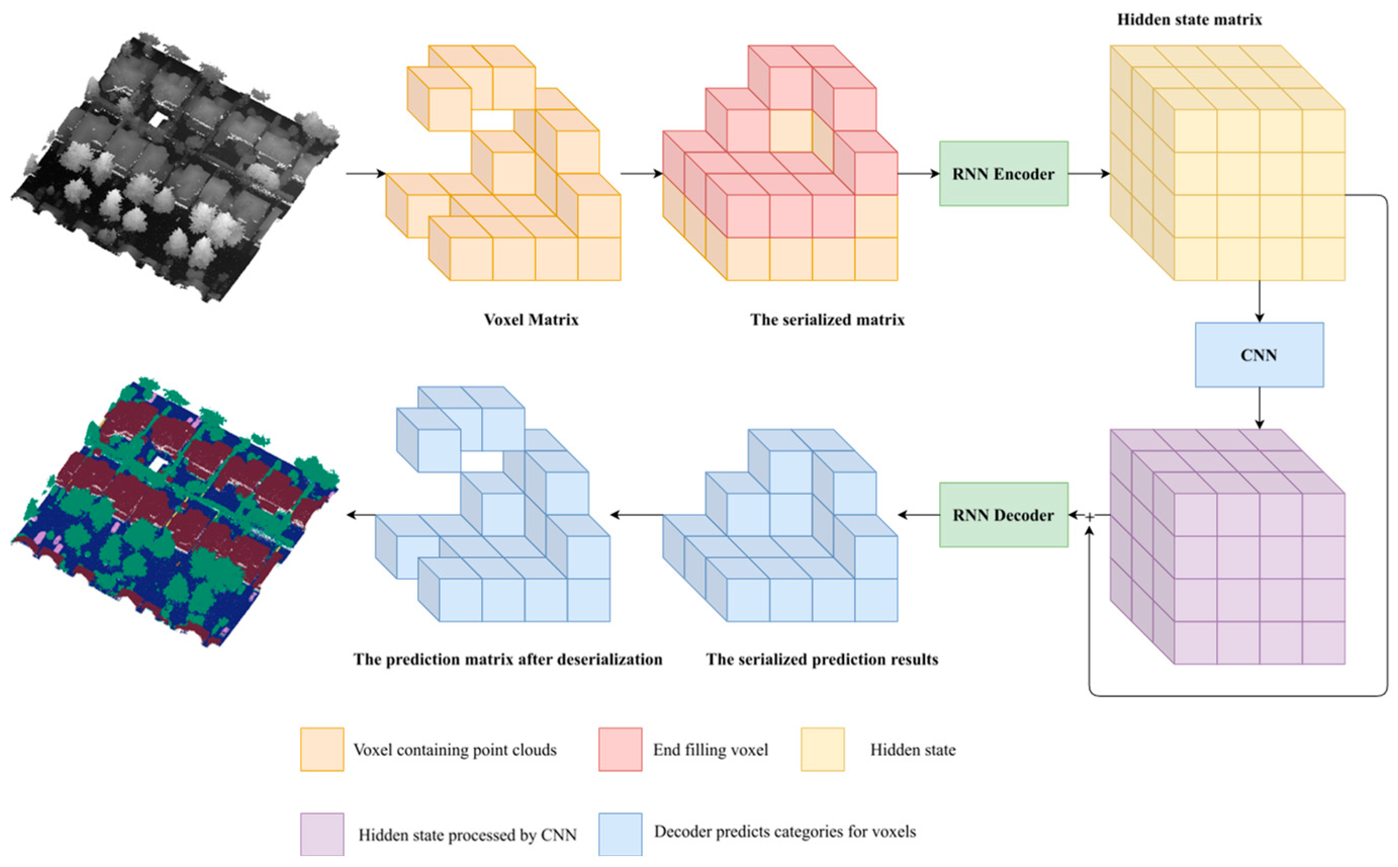
Figure 2.
Serialization and assignment of a voxel matrix of shape [4,3,4]. For clarity, invalid voxels are not drawn, and each row is separated. Since index 0 is used as the elevation for padding voxels, the bottom voxel has a value of 1 instead of 0, and the end voxel's index is the maximum index in the Z-direction plus one (here, 4+1).
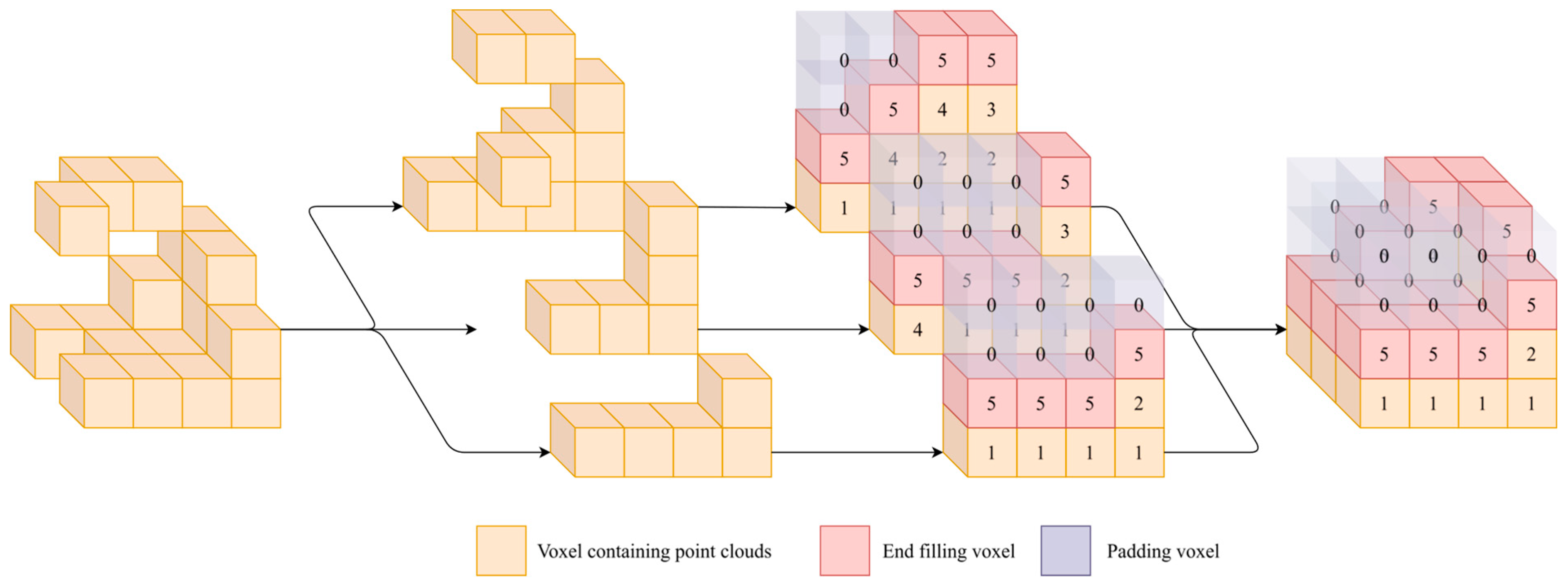
Figure 3.
Encoding process of a spatial sequence (1,2,5,0). Each elevation is embedded into an n-dimensional vector, and the RNN encodes these elevation vectors sequentially, ultimately storing all information in a fixed-length m-dimensional hidden state vector. Thus, the RNN achieves selective retention of elevation information and maps it into a structured m-dimensional vector.
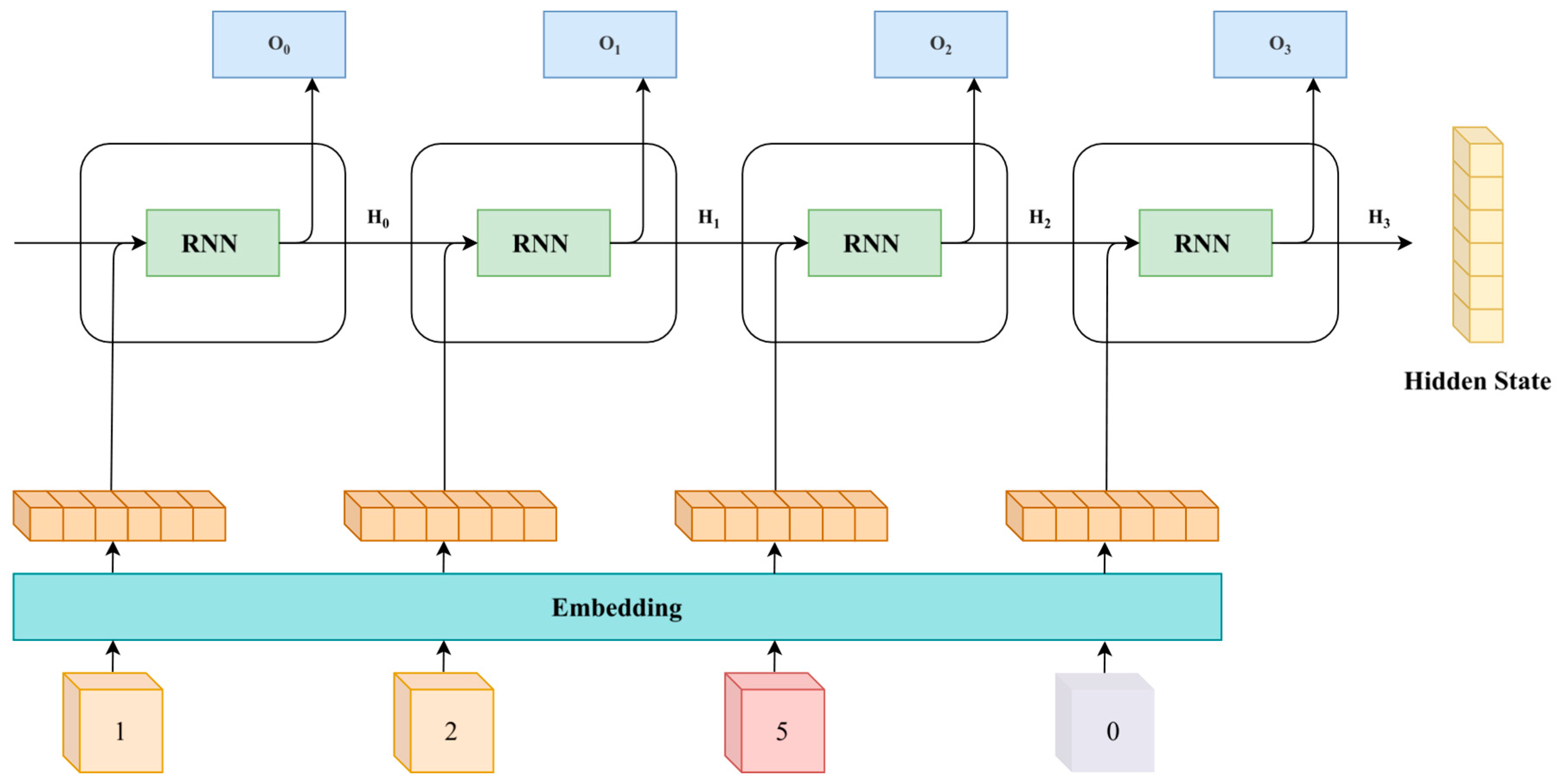
Figure 5.
Prediction process of the SeqConv-Net structure. The decoder is initialized with the hidden state output by the encoder, and the first prediction uses a special Start token. Subsequently, the hidden state is updated, and the previous output is concatenated with the last layer's hidden state as the next input for continuous prediction.
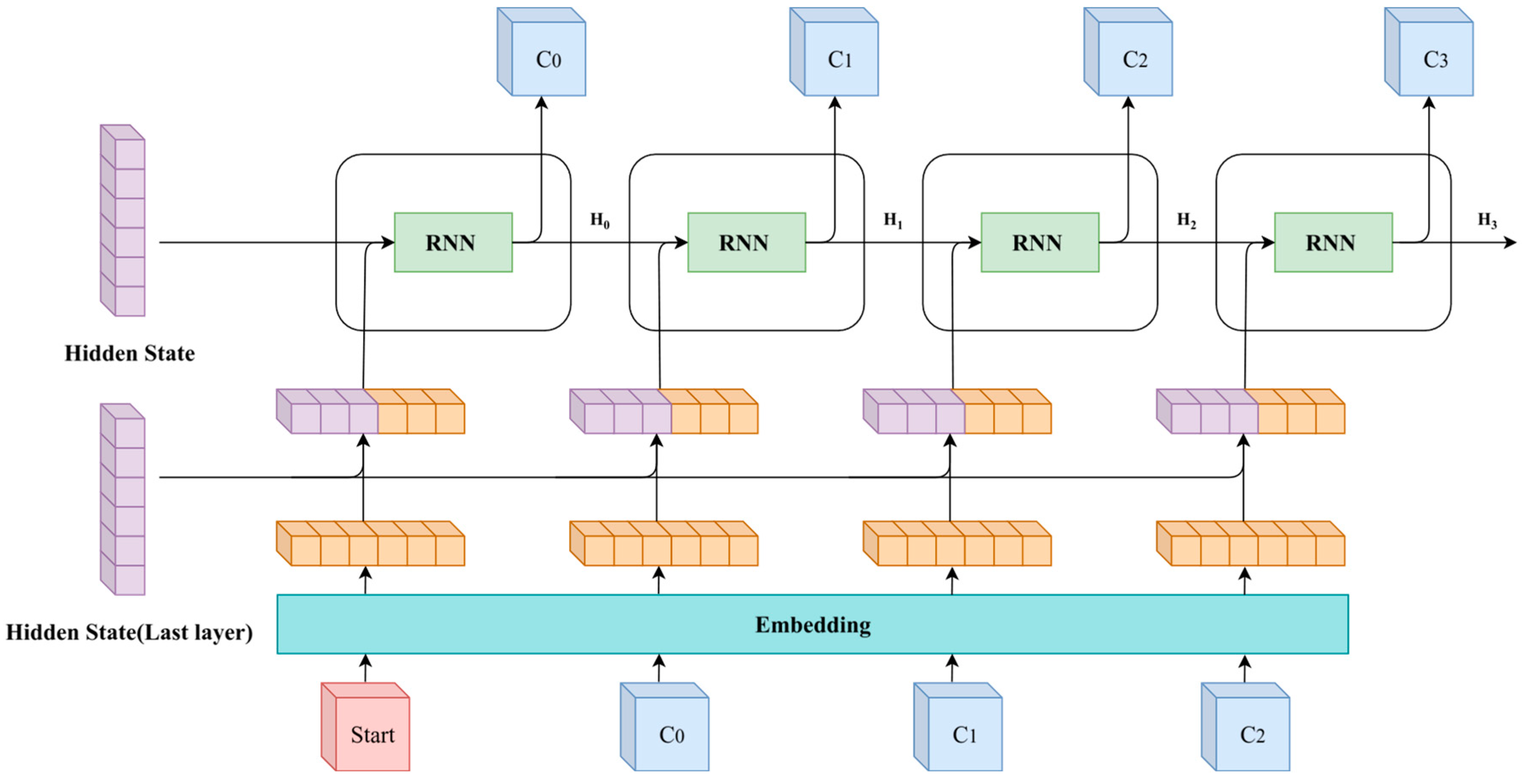
Figure 6.
Accuracy loss after deserialization at different resolutions.
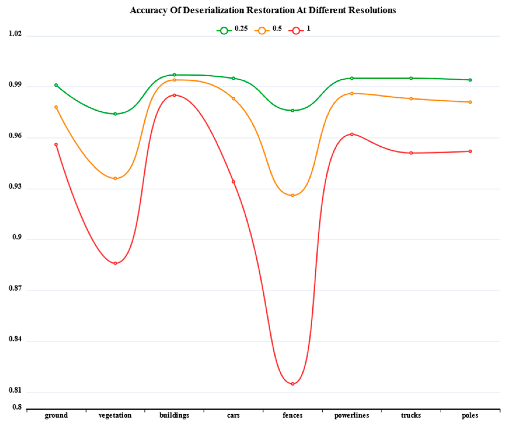
Figure 7.
Impact of truncation on model prediction. The truncation surface is marked with a red ellipse. Due to the vertical continuity of objects, points on the truncation surface often have the same category as the truncation point. Therefore, the truncation method allows the network to predict all voxels in the sequence even if it cannot input the entire sequence.
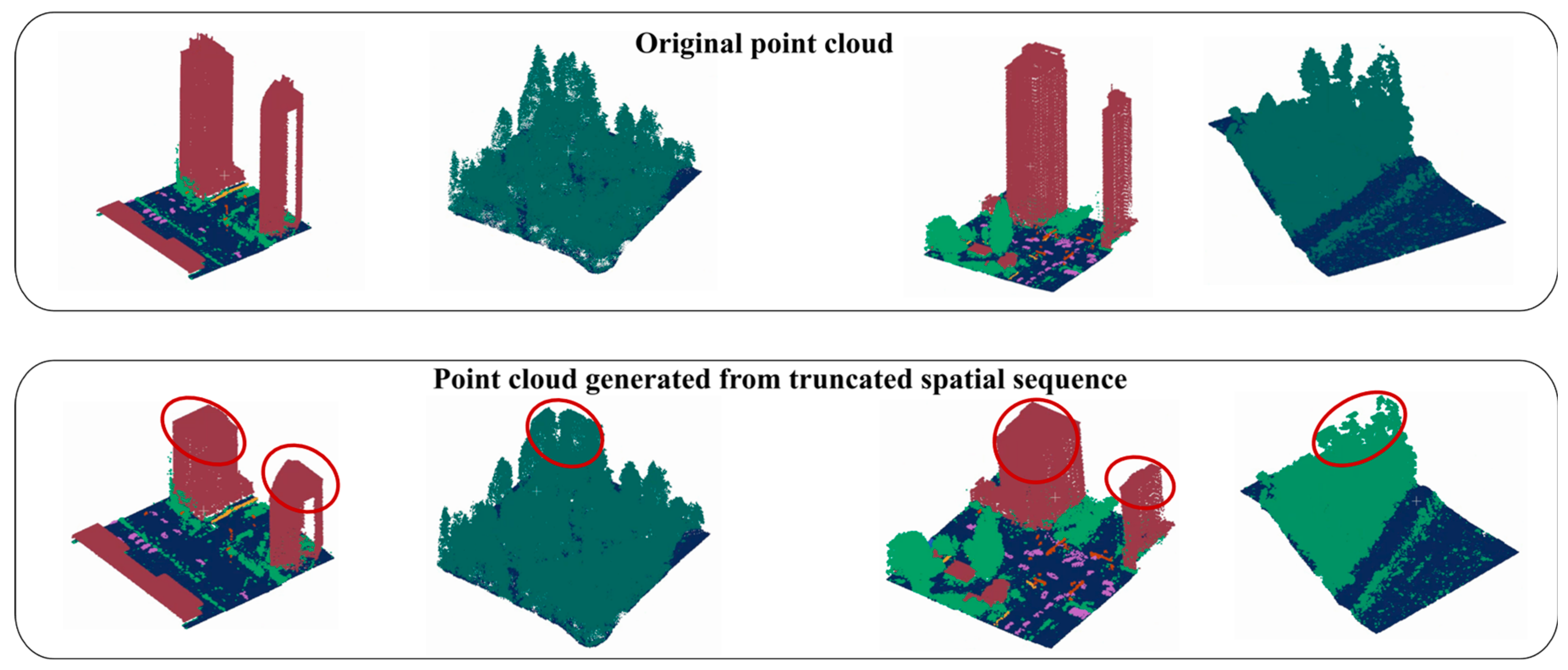
Figure 9.
GRU-UNet segmentation model. The encoder and decoder use two layers of GRU.
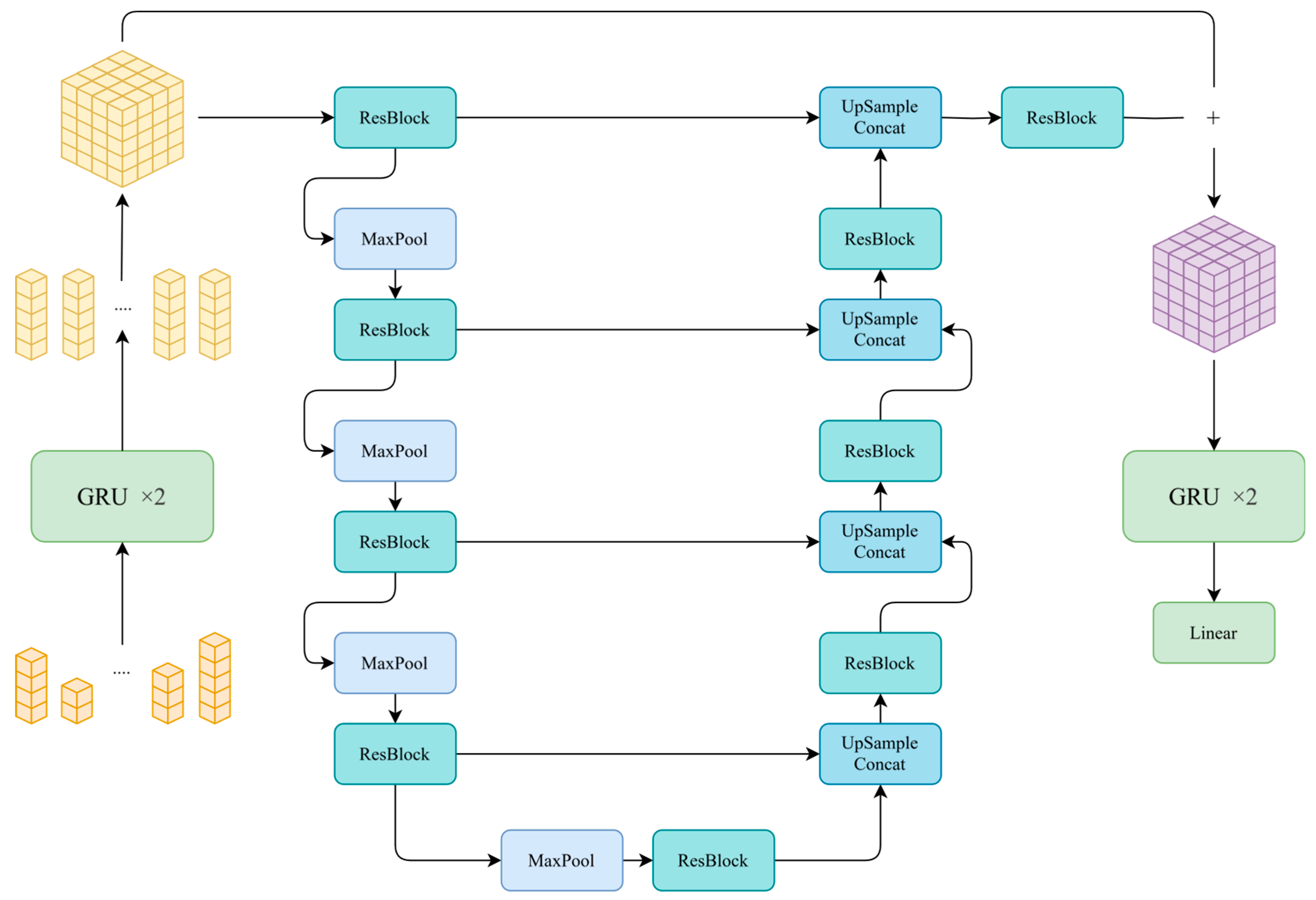
Figure 12.
16-channel images composed of 16-dimensional hidden variables. It can be observed that the channels exhibit some degree of correspondence with the DSM.
Figure 12.
16-channel images composed of 16-dimensional hidden variables. It can be observed that the channels exhibit some degree of correspondence with the DSM.
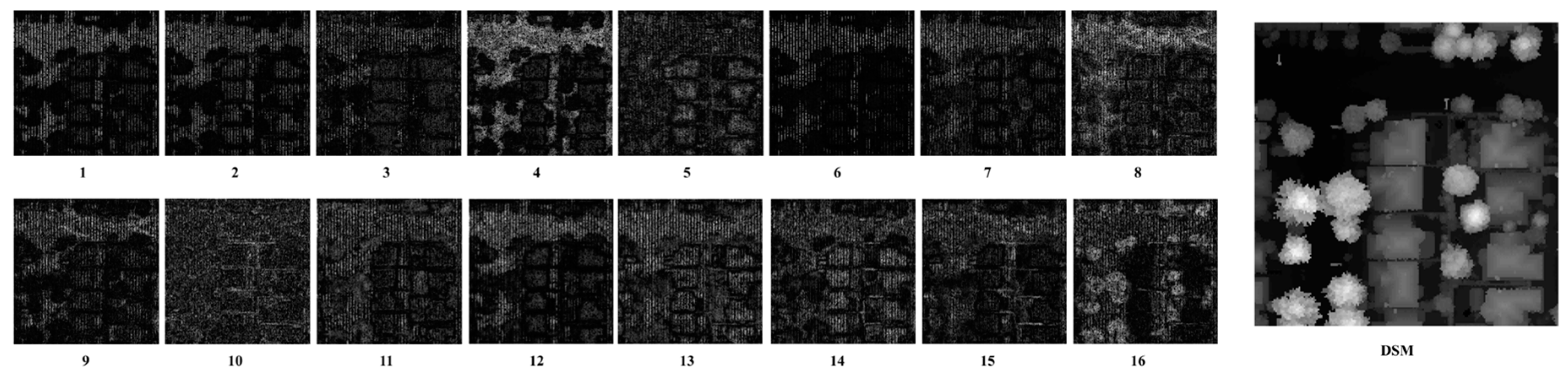
Table 1.
IOU precision after label deserialization.
| Resolution | ground | vegetation | buildings | cars | fences | powerlines | trucks | poles | mIOU |
| 0.25 | 0.991 | 0.974 | 0.997 | 0.995 | 0.976 | 0.995 | 0.995 | 0.994 | 0.990 |
| 0.5 | 0.978 | 0.936 | 0.994 | 0.983 | 0.926 | 0.986 | 0.983 | 0.981 | 0.971 |
| 1 | 0.956 | 0.886 | 0.985 | 0.934 | 0.815 | 0.962 | 0.951 | 0.952 | 0.930 |
Table 2.
IOU Accuracy After Deserialization With and Without Truncation.
| Truncation | ground | vegetation | cars | trucks | powerlines | fences | poles | buildings | mIOU |
| NO | 0.915 | 0.943 | 0.927 | 0.977 | 0.955 | 0.828 | 0.973 | 0.990 | 0.938 |
| YES | 0.915 | 0.943 | 0.927 | 0.977 | 0.955 | 0.828 | 0.973 | 0.990 | 0.938 |
Table 3.
mIOU Accuracy and Speed of Different Models.
| Method | input points | mIOU | Speed |
| PointNet++ | 8192 | 0.683 | 726.6s |
| KPConv | 8192 | 0.726 | 186.9s |
| DGCNN | 8192 | 0.665 | 203.2s |
| PointCNN | 8192 | 0.584 | - |
| SPG | 8192 | 0.606 | - |
| ConvPoint | 8192 | 0.674 | - |
| PointTransformer | 8192 | 0.749 | 698.7s |
| PReFormer | 8192 | 0.709 | - |
| PointMamba | 8192 | 0.733 | 90.7s |
| PointCloudMamba | 8192 | 0.747 | 115.6s |
| Ours | - | 0.755 | 4.01s |
Disclaimer/Publisher’s Note: The statements, opinions and data contained in all publications are solely those of the individual author(s) and contributor(s) and not of MDPI and/or the editor(s). MDPI and/or the editor(s) disclaim responsibility for any injury to people or property resulting from any ideas, methods, instructions or products referred to in the content. |
© 2025 by the authors. Licensee MDPI, Basel, Switzerland. This article is an open access article distributed under the terms and conditions of the Creative Commons Attribution (CC BY) license (http://creativecommons.org/licenses/by/4.0/).
Copyright: This open access article is published under a Creative Commons CC BY 4.0 license, which permit the free download, distribution, and reuse, provided that the author and preprint are cited in any reuse.


