

Submitted:
19 April 2025
Posted:
21 April 2025
You are already at the latest version
Abstract
This study investigates the long-run relationship between green finance and the ecological footprint in 13 countries with the highest levels of green financial development, while also examining the roles of green growth, economic growth, financial globalization, and capital formation. Using panel data from 1992 to 2020, the analysis applies advanced econometric techniques, including the Augmented Mean Group (AMG), Fully Modified Ordinary Least Squares (FMOLS), and Dynamic Ordinary Least Squares (DOLS) estimators to identify long-term effects. In addition, the Dumitrescu-Hurlin panel bootstrap causality test is used to explore the direction of relationships among variables. The results confirm the existence of cointegration among all variables. Green finance and green growth are found to reduce the ecological footprint, indicating their effectiveness in mitigating environmental degradation. In contrast, economic growth, financial globalization, and capital formation contribute positively to the ecological footprint, suggesting a link to increased environmental pressure. The causality analysis reveals a bidirectional relationship between green growth and ecological footprint, while green finance, economic growth, financial globalization, and capital are found to be causal factors of ecological footprint. The findings highlight the importance of promoting green finance and sustainable growth strategies while ensuring that financial and capital flows support environmental objectives.
Keywords:
Green Finance
; Ecological Footprint
; Environmental Sustainability
; Financial Development
; Financial Globalization
; Green Growth
; China
; USA
1. Introduction
Climate change, global warming, environmental degradation, and increasing environmental concerns have led academics, policymakers, and many stakeholders to maintain a strong focus on sustainable development—particularly its environmental sustainability component [1] [2] [3] [4] [5]. The United Nations COP-27 conference, emphasizing key goals such as climate finance, carbon neutrality, and sustainable growth, aims to reduce the global temperature by 1.5 degrees Celsius and achieve the 2030 sustainable development targets [6]. In line with this and earlier international conferences, conventions, and summits on environmental protection, the world is taking rapid steps toward building a greener and more sustainable economy.
Against this backdrop, green finance is recognized as one of the most crucial factors in achieving a sustainable environment and development [7] [8] [9]. Green finance encompasses financial products and services—such as green bonds, green loans, and carbon pricing—that promote environmentally friendly initiatives, sustainable development, and environmental sustainability [10]. A key characteristic that differentiates green finance from other types of finance is its focus on channeling public- and private-sector funds toward green entrepreneurs who foster sustainable development and improve the environment [11].
Research addressing green finance often centers on its determinants or its impacts. In one strand of the literature, scholars examine the factors driving green finance [12] [13] [14]. Another strand explores the effects of green finance, highlighting, for instance, how it guides financial resources into renewable energy investments and projects, thereby helping develop that sector [15]. The diversification and growth of green financial products—such as green funds and insurance—can also foster and enhance green innovations [16]. Moreover, green finance improves energy efficiency by reducing excessive energy inputs that contribute to environmental pollution, supports the green manufacturing sector by boosting green total factor productivity [17], and positively influences employment and new business creation by promoting effective resource use [18]. Because green finance and related strategies can affect the supply, demand, and availability of natural resources such as coal, oil, and natural gas, some researchers claim a positive relationship between a country’s (green) financial development and its natural resources [19]. Finally, green loans—an important subset of green finance—can advance green economic growth by strengthening the financial performance of banks and other financial institutions and channeling capital to green entrepreneurs [20].
In recent years, several studies have examined the relationship between green finance and environmental degradation or environmental sustainability [21] [8] [22] [23] [24]. Because financial institutions direct some of their loans and funds toward green projects and investments, green finance can be viewed as an important tool to combat environmental pollution. Sharif et al. [21], Wei and Bai [9], and Li [24] find that green finance bolsters environmental sustainability by reducing CO2 emissions, whereas Numan et al. [22] report that green finance curbs environmental pollution by lowering the ecological footprint. Taken together, these results suggest that green financial practices can play a significant role in designing environmental policy. Green economic growth—an integral element of a sustainable environment—also helps reduce pollution [25], a finding corroborated by Hao et al. [26], Dong et al. [27], and Li [24]. Meanwhile, researchers highlight that the growing or diminishing effect of financial globalization on environmental degradation remains a topic of debate [28]. Some studies posit that economic growth and capital formation create a scale effect in the economy, increase energy demand, and exacerbate pollution [29] [30]. Consequently, because these variables often appear in environmental pollution regressions, they too warrant policy consideration alongside green finance.
This study analyzes the relationship between green finance and the ecological footprint from 1990 to 2019 across 13 countries identified as leaders in green financial development. According to the IFF Global Finance and Development Report [31], France, the UK, Germany, China, the Netherlands, Japan, Sweden, Denmark, Spain, the USA, Norway, Austria, and Italy rank highest in the Global Finance and Development Index, making them ideal subjects for studying the impact of green finance. Except for China, all are OECD members. These nations also perform strongly on the OECD green growth indicators (e.g., CO2 productivity and energy productivity) for 2021 [32]. Nevertheless, in terms of environmental pollution, China remains the world’s largest emitter of greenhouse gases, and OECD countries also display high emission levels. Specifically, while total global CO2 emissions in 2021 were 33,9 billion tons, the collective OECD total reached 11,3 billion tons—accounting for 34% of the global figure. Meanwhile, China alone produced 30% of total CO2 emissions [33]. Regarding ecological footprint, China leads with 5,1 billion global hectares, followed by the USA (2,1 billion global hectares) and Japan (533 million global hectares). Many of the remaining countries likewise rank high. These data underscore that policies aimed at reducing environmental pollution and enhancing environmental sustainability remain urgent for these nations.
In light of the above, this study explores several research questions: (1) Can green finance help combat environmental pollution by reducing the ecological footprint? (2) Does green economic growth reduce environmental pollution through its impact on the ecological footprint? (3) What roles do economic growth, financial globalization, and capital formation play in shaping the ecological footprint? (4) Given the results, what effective policies might help curb environmental pollution?
The study makes several contributions to the literature. First, it examines the impact of green finance on the ecological footprint while integrating green economic growth, financial globalization, economic growth, and capital formation as control variables, a combination rarely explored together. Second, it focuses on the 13 countries with the strongest green financial development—an understudied group in previous analyses. Third, it uses ecological footprint as an environmental sustainability metric, which is a more comprehensive measure of environmental degradation incorporating the planet’s biocapacity. Fourth, the study employs the Augmented Mean Group (AMG) estimator, a dynamic panel method that yields robust results even under slope heterogeneity and cross-sectional dependence. It also applies the Dumitrescu-Hurlin bootstrap causality test, which is seldom used in many panel studies, thereby providing more reliable causal insights for policy recommendations. Finally, by modeling green growth, financial globalization, economic growth, and capital formation, the study explains multiple causes of environmental degradation and can help inform a wide range of policies to mitigate it.
2. Literature Review
This study examines how green finance, green growth, economic growth, financial globalization, and capital formation affect the ecological footprint. The following subsections provide a review of the relevant literature on each variable’s relationship with environmental degradation.
2.1. Green Finance and Environmental Degradation
Green finance, which links ecological and financial considerations, is widely regarded as pivotal for environmental protection [34]. In recent years, it has gained attention as a tool to restore ecological balance and curb pollution [34] [35] [15] [22]. Feng et al. [36] posit that in China, expanding green bonds—an important component of green finance—helps reduce environmental pollution by incentivizing renewable energy investments, whereas contracting green bonds exacerbates pollution by reducing such investments. Glomsrød and Wei [37] estimate that green finance could cut global coal consumption by approximately 2.5% by 2030, increasing the share of electricity from renewable energy sources from 42% to 46%, although effects vary across countries or regions. Collectively, these insights support the hypothesis that green finance prevents environmental degradation.
Several empirical studies corroborate this viewpoint. Li et al. [15] find that in MINT countries, green finance alleviates environmental degradation, with a particular emphasis on ecological sustainability measures such as renewable energy, natural resources, and energy innovation. Chin et al. [35] observe a negative relationship between green finance and environmental pollution in BRI countries, while Numan et al. [22], employing the Driscoll-Kraay estimator for 13 countries, report that green finance constrains environmental degradation. These findings align with those of Sharif et al. [21], Wei and Bai [9], Li [38] , and Umar and Safi [39], collectively suggesting that green finance is a powerful mechanism for protecting the environment.
2.2. Green Growth and Environmental Degradation
When a country’s income rises, higher economic growth often leads to increased energy consumption and CO₂ emissions, posing a threat to environmental quality [40]. Consequently, many nations are shifting their development strategies toward green growth, which can mitigate the adverse effects of long-term economic expansion by minimizing environmental hazards [41]. D’amato and Korhonen [42] advocate green growth as a critical strategy for achieving environmental sustainability. Similarly, Wu et al. [40] and Ahmad and Wu [43] suggest that by bridging environmental priorities and economic objectives, green growth helps prevent environmental degradation. Thus emerges the hypothesis that green growth reduces environmental degradation.
Empirical research provides supportive evidence. Oyebanji et al. [44] demonstrate that green growth in Nigeria improves environmental quality by reducing pollution. Hao et al. [26] , examining G7 countries, find a negative association between green growth and environmental degradation, implying that green growth contributes to a sustainable environment. Dong et al. [27] highlight similar pollution-curbing effects in their study of 30 cities in China. Ahmad and Wu [43], applying PQR, FMOLS, and DOLS estimators to data from 20 OECD countries, show that green growth fosters ecological sustainability by decreasing the ecological footprint. Saqib et al. [45] also report that among the 10 countries with the highest ecological footprint, green growth effectively mitigates environmental degradation—results consistent with findings in Gu et al. [46] and Lin and Ullah [25].
2.3. Economic Growth and Environmental Degradation
Economic growth can undermine environmental quality by amplifying raw material use and energy consumption, thereby increasing pollution [47]. In this regard, economic growth can fuel the scale effect, where higher production heightens environmental degradation [48]. Numerous studies investigate the link between economic growth and environmental outcomes [50], generally supporting the hypothesis that economic growth causes environmental degradation.
Shahbaz et al. [48], analyzing the 10 countries with the largest ecological footprints, conclude via the CCE estimator that financial development and economic growth both increase the ecological footprint. Alola et al. [51], in a study of 16 European countries, and Kongbuamai et al. [50], examining ASEAN nations, similarly find that economic growth exacerbates the ecological footprint. Awosusi et al. [47] show that as economies grow, environmental degradation accelerates. Danish et al. [49] reach a parallel conclusion for Pakistan using the ARDL model, suggesting that economic growth reduces environmental quality by expanding the ecological footprint.
2.4. Financial Globalization and Environmental Degradation
Financial globalization can offer capital essential for technological advancement, innovation, and renewable energy investments, potentially reducing environmental degradation over the long term [52]. Conversely, in countries with lax environmental regulations, increased financial flows may fund polluting energy projects, prioritizing financial returns over ecological concerns and thereby accelerating environmental deterioration [53]. Meanwhile, globalization can also drive economic transformations and spur the adoption of green technologies, enhancing productivity and reducing pollution [54]. Based on these contrasting effects, one may hypothesize that financial globalization can either promote or reduce environmental degradation.
Empirical investigations offer mixed results. Kirikkaleli et al. [55] demonstrate that in Turkey, globalization heightens the ecological footprint and thus degrades environmental quality in the long run. Sadiq et al. [52], focusing on BRICS countries, find that financial globalization hinders environmental sustainability by intensifying ecological degradation, whereas nuclear energy and external debt have beneficial effects on ecological stability. By contrast, Miao et al. [56] report that in newly industrializing countries, financial globalization curbs the ecological footprint and enhances environmental quality—an outcome echoed by Awosusi et al. [47] for BRICS countries and Hassan et al. [54] for OECD nations. Wang et al. [53] similarly note that financial globalization can foster environmental degradation, underscoring the complexity of its impacts.
2.5. Capital Formation and Environmental Degradation
Capital formation also influences environmental sustainability [24]. As firms accumulate capital and expand production, they often use more energy and resources, heightening the risk of environmental harm [47]. Li et al. [24] emphasize that rising capital formation can generate a scale effect, enlarging production activities and fueling pollution. Accordingly, it is reasonable to hypothesize that capital formation favors environmental degradation.
Several studies substantiate this link. Baz et al. [57] find that positive shocks in capital formation in Pakistan elevate the ecological footprint, thereby worsening environmental quality. Investigating 17 OECD countries, Mujtaba et al. [30] conclude that economic growth and capital formation both contribute to environmental degradation. Khan and Hou [58], using data from 38 countries, likewise note that increasing capital formation expands the ecological footprint. In research on the G20, Li et al. [24] reach similar conclusions, while Emmanuel et al. [59], studying 101 countries, and Chekouri et al. [60], focusing on Algeria, report parallel findings that elevated capital formation undermines a sustainable environment by raising its ecological footprint.
2.6. Literature Gaps
Existing research generally suggests that green finance and green growth mitigate environmental degradation, while economic growth and capital formation tend to exacerbate it through scale effects; financial globalization shows mixed impacts, either supporting or undermining sustainability depending on regulatory contexts and investment patterns. However, a critical gap remains in that the 13 countries with the highest levels of green financial development—despite their significance—have not been examined collectively as a single case. Additionally, although many studies analyze the relationship between green finance and environmental degradation, few include green growth in the framework; in contrast, the present study positions green finance centrally while also incorporating green growth. Another distinguishing feature is the inclusion of financial globalization—often overlooked in work focusing primarily on green finance, green growth, or environmental degradation.
Moreover, although prior studies (e.g., [23] [35] [36] [22] [21] [13] [39]) address the green finance–ecological sustainability nexus, many omit causality analysis, and almost none employ methods that account for Blomquist-Westerlund slope heterogeneity or the Dumitrescu-Hurlin bootstrap causality approach.
By filling these methodological and contextual gaps—namely, by applying advanced estimators (such as AMG) and integrating green finance, green growth, economic growth, financial globalization, and capital formation into a single environmental pollution model for an understudied cohort—this study offers more robust and comprehensive insights. Through its use of ecological footprint as a holistic measure of environmental sustainability, the analysis paves the way for more targeted sustainability strategies and helps bridge policy shortcomings.
3. Empirical Specification, Data and Methods
3.1. Empirical Specification and Data
This study adopts the ecological footprint as an indicator of environmental pollution because it is a comprehensive measure that covers multiple facets of environmental degradation. Following Ali et al. [61], ecological footprint is expressed in global hectares (gha) per capita. For the independent variables, this study draws on Ahmad et al. [28], Yang et al. [62], and Mujtaba et al. [30] to include green finance, green growth, economic growth, financial globalization, and capital. Specifically, green finance is proxied by the renewable energy public R&D budget (% of total energy public R&D) [46], green growth by CO₂ productivity [63], economic growth by per capita GDP (constant 2015 US dollars) [47], financial globalization by the financial globalization index [64], and capital formation by gross capital formation (% of GDP) [65]. Drawing on these studies, the relationship between EF and the five explanatory variables can be modeled as follows:
where α is the intercept, is the error term, i denotes the cross-sectional units (France, the UK, Germany, China, the Netherlands, Japan, Sweden, Denmark, Spain, the USA, Norway, Austria, and Italy), and t represents the yearly data spanning 1994–2019. The coefficients , , , and capture the long-run elasticities, and all variables are used in their logarithmic form to facilitate elasticity-based interpretations. Table 1 defines and summarizes the key variables.
3.2. Methods
This study employs a multi-step empirical strategy to investigate the relationships. The methodology proceeds with cross-sectional dependence and slope homogeneity tests, unit root tests, cointegration tests, long-run coefficient estimation, and causality analysis (Figure 1.).
The study first tests for cross-sectional dependence and slope homogeneity, as overlooking these properties can lead to biased or inefficient results. To investigate cross-sectional dependence, Pesaran’s CD test [67] is employed, where the null hypothesis posits that there is no dependence among cross-sectional units. For slope homogeneity, the study applies the Δ tests of Pesaran and Yamagata [68] and Blomquist and Westerlund [69], with the null hypothesis indicating homogeneous slopes across the sample.
In the second stage, Pesaran’s CADF test [70] is employed to determine whether the variables are stationary and, if so, at which order of integration. As a second-generation unit root procedure, the CADF test is widely used in panel studies because it provides reliable results under cross-sectional dependence. In the third stage, the possibility of cointegration among the variables is examined using Kao [71], Pedroni [72] , and Westerlund [73] residue-based cointegration tests, as well as Westerlund’s second-generation cointegration test [74] —which features four distinct test statistics. In each of these tests, the null hypothesis states that no cointegration exists among the variables.
After confirming the existence of cointegration, long-term coefficients are estimated and interpreted using the AMG estimator proposed by Bond and Eberhardt [75] , along with the FMOLS and DOLS methods developed by Pedroni [76] [77]. The AMG technique offers several advantages. First, it is considered a second-generation approach suitable for data with cross-sectional dependence and slope heterogeneity. Second, it addresses potential endogeneity issues [78]. Finally, it accommodates variables that are stationary both at level and in first difference. Formally, the AMG procedure begins by estimating the following model with OLS:
Each independent variable’s parameter estimate is derived using the following relationship:
The final stage entails exploring causal relationships among the variables using the Dumitrescu-Hurlin panel bootstrap causality approach, which relies on a bootstrap procedure. This test examines causality by estimating a model of the following form:
This procedure computes W ̅ and Z ̅ test statistics, which are then compared against the bootstrap critical values provided by Dumitrescu and Hurlin [79] to determine whether a causal relationship exists among the variables. Under the null hypothesis, there is no causality, while the alternative hypothesis indicates that causality does exist.
4. Findings and Discussion
This section presents the empirical findings obtained from the methodological procedures outlined above. Specifically, the results seek to answer four key research questions posed in the introduction. To address these questions, the section initially presents the descriptive statistics, the results from cross-sectional dependence and slope homogeneity tests, followed by the outcomes of unit root and cointegration analyses. Subsequently, long-run coefficient estimates from AMG, FMOLS, and DOLS methods are interpreted, and the section concludes with a detailed discussion of causal relationships among the variables and their policy implications.
Table 2 presents descriptive statistics, summarizing key characteristics of the panel dataset utilized in this study, which covers 13 countries over the period from 1992 to 2020. The descriptive statistics inform the subsequent methodological steps by highlighting key characteristics of the dataset that require special consideration. Specifically, the significant deviations from normality identified through the Jarque–Bera test for variables such as lnGF and lnFGL indicate potential outliers or non-linearities. Additionally, the varying levels of skewness and kurtosis, especially the high kurtosis in lnGF and lnFGL, suggest heterogeneity across the panel.
Given these statistical features, the next step of the methodology—testing for cross-sectional dependence and slope homogeneity—is critical. Identifying cross-sectional dependence is important due to potential spillover effects or common shocks across countries, while testing for slope homogeneity is essential to determine whether the relationships among variables differ significantly across countries. Furthermore, these preliminary findings reinforce the necessity of employing second-generation unit root and cointegration tests, as well as robust estimators such as the AMG estimator, which effectively address data heterogeneity, cross-sectional dependence, and potential endogeneity issues identified in the descriptive statistics.
Table 3 presents the correlation matrix illustrating the strength and direction of linear relationships among the variables analyzed. Contrary to theoretical expectations, the results show that green finance (lnGF) and green growth (lnGGDP) exhibit positive correlations with ecological footprint (lnEF), at 0.030 and 0.547, respectively. This finding suggests that, in this preliminary analysis, increases in green finance and green growth unexpectedly coincide with a higher ecological footprint.
On the other hand, the findings align with theoretical predictions for economic growth (lnGDP = 0.415), financial globalization (lnFGL = 0.241), and capital formation (lnCAP = 0.058), which all display positive correlations with ecological footprint. The correlation values among independent variables remain relatively low (all below 0.25), indicating minimal multicollinearity concerns. This supports their combined use in subsequent econometric procedures.
The results of Pesaran’s CD test, used to examine the presence of cross-sectional dependence among the variables, are reported in Table 4. The CD-test statistics and corresponding p-values reveal significant cross-sectional dependence for each variable at the 1% significance level (p-value = 0.000). According to these results, the null hypothesis of no cross-sectional dependence is rejected for all variables, confirming significant cross-sectional dependence within the panel. This implies that a shock occurring in one country can potentially propagate and affect other countries within the panel.
The results of slope homogeneity tests developed by Pesaran and Yamagata and Blomquist and Westerlund are presented in Table 5. According to these findings, the null hypothesis of slope homogeneity is rejected, indicating that slope coefficients differ significantly across countries. This implies that the analysis allows for the use of estimation techniques suitable for heterogeneous panel data, which are capable of capturing variations in slope coefficients across countries—an important consideration given the structural and policy differences among the 13 nations analyzed.
To assess the stationarity properties of the variables, Pesaran’s CADF test is applied under both constant and constant-trend specifications. The unit root test results, presented in Table 6, indicate that none of the variables are stationary at level, but all become stationary after first differencing. This confirms that the variables are integrated of order one, I(1). Establishing the same order of integration across variables is essential for proceeding with cointegration analysis in the next step.
The results of the unit root analysis allowing for the application of the Kao, Pedroni, and Westerlund cointegration tests. The empirical findings, shown in Table 7, provide robust evidence in favor of cointegration among the variables, as the null hypothesis of no cointegration is rejected in most cases. In the Westerlund test, two of the four test statistics—Gt (–9.076, p = 0.000) and Pt (–15.393, p = 0.000)—are statistically significant at the 1% level, indicating strong evidence of cointegration. Although the Ga and Pa statistics are not significant, the significant Gt and Pt values are sufficient to support the presence of a long-run relationship. The additional variance ratio test also supports cointegration at the 5% level (–1.668, p = 0.047).
Similarly, the Pedroni test results show that the Phillips-Perron t-statistic (–8.311) and the Augmented Dickey-Fuller t-statistic (–8.625) are highly significant at the 1% level (p = 0.000), confirming cointegration. Although the modified Phillips-Perron t-statistic is not significant, the strong results from the other two tests reinforce the cointegration evidence. The Kao test further supports these findings, with the modified Dickey-Fuller t-statistic (–5.614), Dickey-Fuller t-statistic (–5.854), and unadjusted Dickey-Fuller t-statistics (–13.518 and –8.145) all significant at the 1% level. Only the Augmented Dickey-Fuller t-statistic (–0.220, p = 0.413) fails to reject the null, but the overall evidence remains overwhelmingly in favor of a long-run relationship.
These results confirm the existence of a cointegrated system among green finance, green growth, economic growth, financial globalization, capital formation, and ecological footprint. This implies that these variables move together over the long term and that any disequilibrium is likely to be temporary. Establishing cointegration justifies the estimation of long-run coefficients and allows for meaningful interpretation of both the direction and magnitude of these relationships.
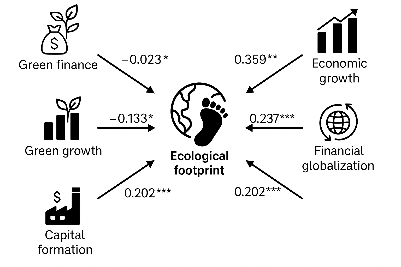
The findings obtained from the AMG estimator, which was applied to estimate the long-run coefficients of the model variables, are presented in Table 8. The coefficient for green finance is found to be –0.023 and statistically significant, indicating that a 1% increase in green finance leads to a 0.023% decrease in the ecological footprint. This result suggests that green finance plays a meaningful role in reducing environmental degradation, reinforcing its position as an environmentally friendly financial mechanism.
This outcome implies that the countries included in the study have made significant progress in green financial development, actively prioritizing environmentally responsible financing practices as a means of addressing ecological challenges. The finding aligns with theoretical expectations and is consistent with previous empirical research. In particular, it supports the results of Tariq and Hassan [80], who examined 70 countries using the GMM approach, and Udeagha and Ngepah [81], who analyzed environmental sustainability determinants in BRICS countries using the CS-ARDL method and Jóźwik et al.[82], who analyzed the USA and leaders of nuclear energy consumers [83] . These parallels reinforce the credibility and generalizability of the current study’s results in the broader literature on green finance and environmental sustainability.
In the long run, the coefficient for green growth is found to be –0.133 and statistically significant, indicating that a 1% increase in green growth leads to a 0.133% reduction in the ecological footprint. This negative relationship suggests that green growth contributes to lowering environmental degradation, confirming the effectiveness of green growth practices in the sampled countries. These findings highlight those policies focused on green growth—such as improving CO₂ productivity, promoting renewable energy efficiency, and adopting cleaner technologies—have yielded substantial environmental benefits. The result is consistent with Lin and Ullah [25], who, using ARDL and DOLS methods, found that green growth reduces CO₂ emissions in Pakistan in both the short and long run. Further support comes from Lin and Ullah [84], who employed the DARDL approach and confirmed a long-run negative relationship between green growth and environmental degradation, reinforcing the present study’s conclusion.
Conversely, the coefficient for economic growth is 0.359 and statistically significant, meaning that a 1% increase in economic growth results in a 0.359% rise in the ecological footprint. This suggests that, for the countries analyzed, higher levels of economic activity are associated with greater environmental pressure. This finding supports the view that economic growth—particularly when driven by industrial production and increased energy consumption—can lead to higher demand for fossil fuels, thus exacerbating environmental degradation. The result aligns with Luo et al. [85], who found that economic growth intensifies environmental pollution in low- and middle-income Asian countries, based on panel MG estimations. However, it contrasts with the findings of Qamri et al. [86], who reported that economic growth reduces environmental pollution in a study of 21 Asian countries, highlighting the regional and structural differences that may influence the nature of this relationship.
Another important long-term finding is that financial globalization has a positive and significant coefficient of 0.237, suggesting that a 1% increase in financial globalization leads to a 0.237% increase in the ecological footprint. This result indicates a positive relationship between financial globalization and environmental degradation, implying that increased financial integration—through foreign direct investment or cross-border capital flows—may be contributing to pollution, especially if financial resources are allocated to high-emission or resource-intensive industries. This outcome highlights a potential unintended consequence of financial openness, where environmental considerations may be secondary to economic or investment objectives. The result is consistent with the findings of Ahmad et al. [87], who, using CS-ARDL and CCEMG techniques, showed that financial globalization negatively impacts environmental quality in G-11 countries.
In addition, the capital formation coefficient is also positive and significant, with a value of 0.202, indicating that a 1% increase in capital leads to a 0.202% increase in the ecological footprint. This result suggests that capital accumulation contributes to environmental degradation by driving up production, industrial activity, and demand for energy—particularly fossil fuels. As capital investment often supports infrastructure and manufacturing expansion, it may unintentionally raise environmental pressure if not directed toward sustainable or low-carbon projects. This finding is in line with the results of Mujtaba et al. [30], who observed a similar relationship in OECD countries, and Li et al. (2023), who reported that capital formation exacerbates ecological footprints in G20 economies. It should be added, however, that Capital formation, particularly through foreign direct investment (FDI), can influence the environment in both positive and negative ways [88]. Together, these results underscore the need for environmentally conscious investment strategies, even in the context of economic development.
The findings of the FMOLS and DOLS estimators, which are employed to verify the robustness of the AMG long-run estimates, are presented in Table 9. Both estimation techniques yield results that are consistent with the AMG findings, thereby reinforcing the reliability and stability of the empirical results. Specifically, green finance and green growth are found to have a negative and significant impact on the ecological footprint, indicating their effectiveness in mitigating environmental degradation. In contrast, economic growth, financial globalization, and capital formation exhibit positive and significant coefficients, confirming their roles in increasing the ecological footprint and contributing to environmental pressure.
Although the AMG, FMOLS, and DOLS estimators provide valuable insights into the long-run effects of each independent variable on the ecological footprint, they do not offer evidence regarding the direction of causality between variables. To address this, the Dumitrescu-Hurlin panel bootstrap causality test is employed, and the results are presented in Table 10.
The causality analysis reveals several important findings. First, there is unidirectional causality running from green finance to the ecological footprint, indicating that changes in green finance Granger-cause changes in environmental sustainability. This result is consistent with Numan et al. [22], who found similar evidence in their study of 13 countries. Second, the results indicate a bidirectional causality between green growth and ecological footprint, suggesting a mutual relationship in which green growth affects environmental outcomes, and environmental pressures may also influence the adoption of green growth strategies. This aligns with the findings of Ahmad and Wu [43] for OECD countries and Lin and Ullah [84], who reported a similar two-way relationship between green growth and CO₂ emissions in Pakistan.
Additionally, the analysis shows that economic growth causes the ecological footprint, confirming that rising income levels contribute to environmental degradation. This result is in line with Bakry et al. [23], who documented a similar causal effect across 76 developing countries. Moreover, a unidirectional causality is identified from financial globalization to ecological footprint, highlighting the environmental consequences of increased financial openness. This finding supports the results of Wang et al. [89], who observed the same direction of causality for countries involved in the One Belt One Road (OBOR) initiative.
Finally, the results show a one-way causality from capital formation to the ecological footprint, suggesting that increases in capital accumulation drive environmental degradation. However, this finding contrasts with Li et al. [24], who found no causal relationship between capital and ecological footprint, indicating that the effect of capital formation on environmental outcomes may vary depending on the country group or methodology used.
5. Conclusion and Policy Implications
Global warming, climate change, and environmental degradation pose serious ecological threats worldwide, underscoring the urgency of pursuing a sustainable environment. In this context, the role of green finance has become increasingly significant. This study investigates the relationship between green finance and the ecological footprint in 13 countries with the highest levels of green financial development, while also examining the impact of green growth, economic growth, financial globalization, and capital on environmental degradation. Long-term effects are estimated using AMG, FMOLS, and DOLS methods, and causality relationships are analyzed with the Dumitrescu-Hurlin panel bootstrap technique.
The findings confirm that all variables are cointegrated. In the long run, green finance and green growth reduce the ecological footprint—and thus environmental degradation—whereas economic growth, financial globalization, and capital exert a positive effect, increasing environmental pressure. The causality analysis shows a bidirectional relationship between green growth and the ecological footprint, while green finance, economic growth, financial globalization, and capital are found to cause the ecological footprint unidirectionally.
These empirical results have direct implications for policymakers. Of particular importance is the observation that green finance and green growth effectively mitigate environmental pollution. As Chin et al. [35] suggest, policymakers can subsidize green loan interest rates, reduce corporate taxes, and establish green loan guarantee schemes. They can also provide green loans to firms for projects that mitigate environmental damage and encourage these companies to adopt environmentally friendly raw materials and green technologies. Expanding the market for green bonds—an essential green finance tool—further supports green growth and enhances environmental quality.
The damage caused by traditional economic growth to the environment elevates the significance of green growth strategies. As emphasized by Mujtaba et al. [30], policymakers should prioritize cleaner investments, provide additional incentives for businesses and industries that generate and use renewable energy, and concentrate on developing ecosystem-friendly renewable energy sources, adhering to a realistic green growth and green economy approach.
Because financial globalization can exacerbate environmental degradation, foreign direct investments and other financial flows—the core components of financial globalization—should be redirected toward ecological innovations and renewable energy, thus mitigating negative environmental impacts. Well-developed financial markets can offer more extensive funding for green initiatives and the transfer and production of eco-friendly technologies. Similarly, measures to minimize the adverse effects of capital formation should be implemented, such as supporting green technological innovations and renewable energy investments in firms with significant capital.
This study focuses on the relationship between green finance and the ecological footprint without including CO₂ emissions or load capacity factor criteria as indicators of environmental degradation. It also excludes determinants like green innovations, economic complexity, institutional quality, and geopolitical risk, which have appeared in recent regression models. Moreover, the sample only includes the 13 countries with the strongest green financial development; consequently, the study does not compare results with countries displaying lower levels of green financial development. Addressing these limitations in future research could facilitate more comprehensive empirical findings and policy recommendations. Methodologically, incorporating CS-ARDL and CS-DL estimators alongside AMG may offer even more robust empirical evidence.
Author Contributions
Conceptualization, B.J., S.S.S., M.D., M.Ç., P.A., A.G.; methodology, S.S.S., M.D., M.Ç.; software, M.D.; formal analysis, S.S.S., M.D., M.Ç.; investigation, B.J., S.S.S., M.D., M.Ç., P.A., A.G.; writing— B.J., S.S.S., M.D., M.Ç., P.A., A.G.; writing—review and editing, B.J., S.S.S., M.D.; visualization, M.Ç., P.A., A.G.; supervision, B.J., S.S.S., M.D.; project administration, B.J., M.D.; funding acquisition, B.J.,. All authors have read and agreed to the published version of the manuscript.
Funding
Please add: The APC was funded by The John Paul II Catholic University of Lublin.
Institutional Review Board Statement
Not applicable.
Informed Consent Statement
Not applicable.
Data Availability Statement
Dataset available on request from the authors.
Conflicts of Interest
The authors declare no conflicts of interest. The funders had no role in the design of the study; in the collection, analyses, or interpretation of data; in the writing of the manuscript; or in the decision to publish the results.
Abbreviations
The following abbreviations are used in this manuscript:
| AMG | Augmented Mean Group |
| CO₂ | Carbon Dioxide |
| CS-ARDL | Cross-Sectionally Augmented Autoregressive Distributed Lag |
| CS-DL | Cross-Sectionally Distributed Lag |
| DOLS | Dynamic Ordinary Least Squares |
| EF | Ecological Footprint |
| FMOLS | Fully Modified Ordinary Least Squares |
| FGL | Financial Globalization |
| GDP | Gross Domestic Product |
| GF | Green Finance |
| GGDP | Green Growth |
| GFN | Global Footprint Network |
| IFF | International Finance Forum |
| KOF | Konjunkturforschungsstelle (Swiss Economic Institute) |
| R&D | Research and Development |
| RMSE | Root Mean Square Error |
| SIC | Schwarz Information Criterion |
| WDI | World Development Indicators |
References
- Khan, S.; Murshed, M.; Ozturk, I.; Khudoykulov, K. The Roles of Energy Efficiency Improvement, Renewable Electricity Production, and Financial Inclusion in Stimulating Environmental Sustainability in the Next Eleven Countries. Renew. Energy 2022, 193, 1164–1176. [Google Scholar] [CrossRef]
- Ma, B.; Sharif, A.; Bashir, M.; Bashir, M.F. The Dynamic Influence of Energy Consumption, Fiscal Policy and Green Innovation on Environmental Degradation in BRICST Economies. Energy Polic. 2023, 183, 113823. [Google Scholar] [CrossRef]
- Sadiq, M.; Moslehpour, M.; Qiu, R.; Hieu, V.M.; Duong, K.D.; Ngo, T.Q. Sharing Economy Benefits and Sustainable Development Goals: Empirical Evidence from the Transportation Industry of Vietnam. J. Innov. Knowl. 2023, 8, 100290. [Google Scholar] [CrossRef]
- Fang, Z. Assessing the Impact of Renewable Energy Investment, Green Technology Innovation, and Industrialization on Sustainable Development: A Case Study of China. Renew. Energy 2023, 205, 772–782. [Google Scholar] [CrossRef]
- Karlilar, S.; Balcilar, M.; Emir, F. Environmental Sustainability in the OECD: The Power of Digitalization, Green Innovation, Renewable Energy and Financial Development. Telecommun. Polic. 2023, 47, 102568. [Google Scholar] [CrossRef]
- Gong, Q.; Ying, L.; Dai, J. Green Finance and Energy Natural Resources Nexus with Economic Performance: A Novel Evidence from China. Resour. Polic. 2023, 84, 103765. [Google Scholar] [CrossRef]
- Cheng, H.; Taghizadeh-Hesary, F. How Green Finance Can Bridge the Energy Poverty Gap: Policies to Mitigate Socioeconomic and Environmental Consequences. Energy Polic. 2023, 182, 113758. [Google Scholar] [CrossRef]
- Hailiang, Z.; Chau, K.Y.; Waqas, M. Does Green Finance and Renewable Energy Promote Tourism for Sustainable Development: Empirical Evidence from China. Renew. Energy 2023, 207, 660–671. [Google Scholar] [CrossRef]
- Wei, X.; Bai, Y. The Role of Green Financing and Natural Resources towards Sustainable Environment: A Comparative Study of US-China. Resour. Polic. 2023, 85, 103922. [Google Scholar] [CrossRef]
- Liu, X.; Zhao, T.; Li, R. Studying the Green Economic Growth with Clean Energy and Green Finance: The Role of Financial Policy. Renew. Energy 2023, 215, 118971. [Google Scholar] [CrossRef]
- Zhang, D.; Chen, X.H.; Lau, C.K.M.; Cai, Y. The Causal Relationship between Green Finance and Geopolitical Risk: Implications for Environmental Management. J. Environ. Manag. 2023, 327, 116949. [Google Scholar] [CrossRef] [PubMed]
- Dan, A.; Tiron-Tudor, A. The Determinants of Green Bond Issuance in the European Union. J. Risk Financial Manag. 2021, 14, 446. [Google Scholar] [CrossRef]
- Sinha, A.; Mishra, S.; Sharif, A.; Yarovaya, L. Does Green Financing Help to Improve Environmental & Social Responsibility? Designing SDG Framework through Advanced Quantile Modelling. J. Environ. Manag. 2021, 292, 112751. [Google Scholar] [CrossRef]
- Xu, Y.; Li, S.; Zhou, X.; Shahzad, U.; Zhao, X. How Environmental Regulations Affect the Development of Green Finance: Recent Evidence from Polluting Firms in China. Renew. Energy 2022, 189, 917–926. [Google Scholar] [CrossRef]
- Li, J.; Dong, K.; Taghizadeh-Hesary, F.; Wang, K. 3G in China: How Green Economic Growth and Green Finance Promote Green Energy? Renew. Energy 2022, 200, 1327–1337. [Google Scholar] [CrossRef]
- Irfan, M.; Razzaq, A.; Sharif, A.; Yang, X. Influence Mechanism between Green Finance and Green Innovation: Exploring Regional Policy Intervention Effects in China. Technol. Forecast. Soc. Chang. 2022, 182, 121882. [Google Scholar] [CrossRef]
- Tong, L.; Jabbour, C.J.C.; belgacem, S. ben; Najam, H.; Abbas, J. Role of Environmental Regulations, Green Finance, and Investment in Green Technologies in Green Total Factor Productivity: Empirical Evidence from Asian Region. J. Clean. Prod. 2022, 380, 134930. [Google Scholar] [CrossRef]
- Jiakui, C.; Abbas, J.; Najam, H.; Liu, J.; Abbas, J. Green Technological Innovation, Green Finance, and Financial Development and Their Role in Green Total Factor Productivity: Empirical Insights from China. J. Clean. Prod. 2023, 382, 135131. [Google Scholar] [CrossRef]
- Asif, M.; Khan, K.B.; Anser, M.K.; Nassani, A.A.; Abro, M.M.Q.; Zaman, K. Dynamic Interaction between Financial Development and Natural Resources: Evaluating the ‘Resource Curse’ Hypothesis. Resour. Polic. 2020, 65, 101566. [Google Scholar] [CrossRef]
- Zhang, D.; Mohsin, M.; Rasheed, A.K.; Chang, Y.; Taghizadeh-Hesary, F. Public Spending and Green Economic Growth in BRI Region: Mediating Role of Green Finance. Energy Polic. 2021, 153, 112256. [Google Scholar] [CrossRef]
- Sharif, A.; Saqib, N.; Dong, K.; Khan, S.A.R. Nexus between Green Technology Innovation, Green Financing, and CO 2 Emissions in the G7 Countries: The Moderating Role of Social Globalisation. Sustain. Dev. 2022, 30, 1934–1946. [Google Scholar] [CrossRef]
- Numan, U.; Ma, B.; Sadiq, M.; Bedru, H.D.; Jiang, C. The Role of Green Finance in Mitigating Environmental Degradation: Empirical Evidence and Policy Implications from Complex Economies. J. Clean. Prod. 2023, 400, 136693. [Google Scholar] [CrossRef]
- Bakry, W.; Mallik, G.; Nghiem, X.-H.; Sinha, A.; Vo, X.V. Is Green Finance Really “Green”? Examining the Long-Run Relationship between Green Finance, Renewable Energy and Environmental Performance in Developing Countries. Renew. Energy 2023, 208, 341–355. [Google Scholar] [CrossRef]
- Li, Y.; Wang, X.; Imran, A.; Aslam, M.U.; Mehmood, U. Analyzing the Contribution of Renewable Energy and Natural Resources for Sustainability in G-20 Countries: How Gross Capital Formation Impacts Ecological Footprints. Heliyon 2023, 9, e18882. [Google Scholar] [CrossRef]
- Lin, B.; Ullah, S. Towards the Goal of Going Green: Do Green Growth and Innovation Matter for Environmental Sustainability in Pakistan. Energy 2023, 285, 129263. [Google Scholar] [CrossRef]
- Hao, L.-N.; Umar, M.; Khan, Z.; Ali, W. Green Growth and Low Carbon Emission in G7 Countries: How Critical the Network of Environmental Taxes, Renewable Energy and Human Capital Is? Sci. Total Environ. 2021, 752, 141853. [Google Scholar] [CrossRef]
- Dong, K.; Wang, B.; Zhao, J.; Taghizadeh-Hesary, F. Mitigating Carbon Emissions by Accelerating Green Growth in China. Econ. Anal. Polic. 2022, 75, 226–243. [Google Scholar] [CrossRef]
- Ahmad, M.; Jiang, P.; Murshed, M.; Shehzad, K.; Akram, R.; Cui, L.; Khan, Z. Modelling the Dynamic Linkages between Eco-Innovation, Urbanization, Economic Growth and Ecological Footprints for G7 Countries: Does Financial Globalization Matter? Sustain. Cities Soc. 2021, 70, 102881. [Google Scholar] [CrossRef]
- Hussain, M.; Dogan, E. The Role of Institutional Quality and Environment-Related Technologies in Environmental Degradation for BRICS. J. Clean. Prod. 2021, 304, 127059. [Google Scholar] [CrossRef]
- Mujtaba, A.; Jena, P.K.; Bekun, F.V.; Sahu, P.K. Symmetric and Asymmetric Impact of Economic Growth, Capital Formation, Renewable and Non-Renewable Energy Consumption on Environment in OECD Countries. Renew Sustain Energy Rev 2022, 160, 112300. [Google Scholar] [CrossRef]
- (IFF), I.F.F. Global Finance and Development Report 2021; IFF: Beijing, 2021.
- Green Growth Indicators. OECD Environ. Stat. [CrossRef]
- BP BP Statistical Review of World Energy 2022; BP, 2022.
- Wang, Y.; Zhi, Q. The Role of Green Finance in Environmental Protection: Two Aspects of Market Mechanism and Policies. Energy Procedia 2016, 104, 311–316. [Google Scholar] [CrossRef]
- Chin, M.-Y.; Ong, S.-L.; Ooi, D.B.-Y.; Puah, C.-H. The Impact of Green Finance on Environmental Degradation in BRI Region. Environ., Dev. Sustain. 2022, 1–16. [CrossRef]
- Feng, Y.; Xiao, Z.; Zhou, J.; Ni, G. Asymmetrically Examining the Impact of Green Finance and Renewable Energy Consumption on Environmental Degradation and Renewable Energy Investment: The Impact of the COVID-19 Outbreak on the Chinese Economy. Energy Rep. 2023, 9, 5458–5472. [Google Scholar] [CrossRef]
- Glomsrød, S.; Wei, T. Business as Unusual: The Implications of Fossil Divestment and Green Bonds for Financial Flows, Economic Growth and Energy Market. Energy Sustain. Dev. 2018, 44, 1–10. [Google Scholar] [CrossRef]
- Li, Z. Do Geopolitical Risk, Green Finance, and the Rule of Law Affect the Sustainable Environment in China? Findings from the BARDL Approach. Resour. Polic. 2023, 81, 103403. [Google Scholar] [CrossRef]
- Umar, M.; Safi, A. Do Green Finance and Innovation Matter for Environmental Protection? A Case of OECD Economies. Energy Econ. 2023, 119, 106560. [Google Scholar] [CrossRef]
- Wu, H.; Ren, S.; Yan, G.; Hao, Y. Does China’s Outward Direct Investment Improve Green Total Factor Productivity in the “Belt and Road” Countries? Evidence from Dynamic Threshold Panel Model Analysis. J. Environ. Manag. 2020, 275, 111295. [Google Scholar] [CrossRef]
- Zhou, G.; Zhu, J.; Luo, S. The Impact of Fintech Innovation on Green Growth in China: Mediating Effect of Green Finance. Ecol. Econ. 2022, 193, 107308. [Google Scholar] [CrossRef]
- D’Amato, D.; Korhonen, J. Integrating the Green Economy, Circular Economy and Bioeconomy in a Strategic Sustainability Framework. Ecol. Econ. 2021, 188, 107143. [Google Scholar] [CrossRef]
- Ahmad, M.; Wu, Y. Combined Role of Green Productivity Growth, Economic Globalization, and Eco-Innovation in Achieving Ecological Sustainability for OECD Economies. J. Environ. Manag. 2022, 302, 113980. [Google Scholar] [CrossRef]
- J. , O.I.; Adeniyi, B.; Hlalefang, K.; P., L.R. Green Growth and Environmental Sustainability in Nigeria. International Journal of Energy Economics and Policy 2017, 4, 216–223. [Google Scholar]
- Saqib, N.; Usman, M.; Ozturk, I.; Sharif, A. Harnessing the Synergistic Impacts of Environmental Innovations, Financial Development, Green Growth, and Ecological Footprint through the Lens of SDGs Policies for Countries Exhibiting High Ecological Footprints. Energy Polic. 2024, 184, 113863. [Google Scholar] [CrossRef]
- Gu, X.; Shen, X.; Zhong, X.; Wu, T.; Rahim, S. Natural Resources and Undesired Productions of Environmental Outputs as Green Growth: EKC in the Perspective of Green Finance and Green Growth in the G7 Region. Resour. Polic. 2023, 82, 103552. [Google Scholar] [CrossRef]
- Awosusi, A.A.; Adebayo, T.S.; Altuntaş, M.; Agyekum, E.B.; Zawbaa, H.M.; Kamel, S. The Dynamic Impact of Biomass and Natural Resources on Ecological Footprint in BRICS Economies: A Quantile Regression Evidence. Energy Rep. 2022, 8, 1979–1994. [Google Scholar] [CrossRef]
- Shahbaz, M.; Dogan, M.; Akkus, H.T.; Gursoy, S. The Effect of Financial Development and Economic Growth on Ecological Footprint: Evidence from Top 10 Emitter Countries. Environ. Sci. Pollut. Res. 2023, 30, 73518–73533. [Google Scholar] [CrossRef]
- Danish; Hassan, S. T.; Baloch, M.A.; Mahmood, N.; Zhang, J. Linking Economic Growth and Ecological Footprint through Human Capital and Biocapacity. Sustain. Cities Soc. 2019, 47, 101516. [Google Scholar] [CrossRef]
- Kongbuamai, N.; Bui, Q.; Yousaf, H.M.A.U.; Liu, Y. The Impact of Tourism and Natural Resources on the Ecological Footprint: A Case Study of ASEAN Countries. Environ. Sci. Pollut. Res. 2020, 27, 19251–19264. [Google Scholar] [CrossRef]
- Alola, A.A.; Bekun, F.V.; Sarkodie, S.A. Dynamic Impact of Trade Policy, Economic Growth, Fertility Rate, Renewable and Non-Renewable Energy Consumption on Ecological Footprint in Europe. Sci. Total Environ. 2019, 685, 702–709. [Google Scholar] [CrossRef]
- Sadiq, M.; Shinwari, R.; Usman, M.; Ozturk, I.; Maghyereh, A.I. Linking Nuclear Energy, Human Development and Carbon Emission in BRICS Region: Do External Debt and Financial Globalization Protect the Environment? Nucl Eng Technol 2022, 54, 3299–3309. [Google Scholar] [CrossRef]
- Wang, B.; Yan, C.; Iqbal, N.; Fareed, Z.; Arslan, A. Impact of Human Capital and Financial Globalization on Environmental Degradation in OBOR Countries: Critical Role of National Cultural Orientations. Environ. Sci. Pollut. Res. 2022, 29, 37327–37343. [Google Scholar] [CrossRef]
- Hassan, S.T.; Batool, B.; Wang, P.; Zhu, B.; Sadiq, M. Impact of Economic Complexity Index, Globalization, and Nuclear Energy Consumption on Ecological Footprint: First Insights in OECD Context. Energy 2023, 263, 125628. [Google Scholar] [CrossRef]
- Kirikkaleli, D.; Adebayo, T.S.; Khan, Z.; Ali, S. Does Globalization Matter for Ecological Footprint in Turkey? Evidence from Dual Adjustment Approach. Environ. Sci. Pollut. Res. 2020, 28, 14009–14017. [Google Scholar] [CrossRef] [PubMed]
- Miao, Y.; Razzaq, A.; Adebayo, T.S.; Awosusi, A.A. Do Renewable Energy Consumption and Financial Globalisation Contribute to Ecological Sustainability in Newly Industrialized Countries? Renew. Energy 2022, 187, 688–697. [Google Scholar] [CrossRef]
- Baz, K.; Xu, D.; Ali, H.; Ali, I.; Khan, I.; Khan, M.M.; Cheng, J. Asymmetric Impact of Energy Consumption and Economic Growth on Ecological Footprint: Using Asymmetric and Nonlinear Approach. Sci. Total Environ. 2020, 718, 137364. [Google Scholar] [CrossRef] [PubMed]
- Khan, I.; Hou, F.; Zakari, A.; Tawiah, V.K. The Dynamic Links among Energy Transitions, Energy Consumption, and Sustainable Economic Growth: A Novel Framework for IEA Countries. Energy 2021, 222, 119935. [Google Scholar] [CrossRef]
- Emmanuel, O.N.B.; Fonchamnyo, D.C.; Thierry, M.A.; Dinga, G.D. Ecological Footprint in a Global Perspective: The Role of Domestic Investment, FDI, Democracy and Institutional Quality. J. Glob. Responsib. 2023, 14, 431–451. [Google Scholar] [CrossRef]
- Chekouri, S.M.; Chibi, A.; Benbouziane, M. The Impact of Natural Resource Abundance on Ecological Footprint: Evidence from Algeria. Environ. Sci. Pollut. Res. 2023, 30, 69289–69306. [Google Scholar] [CrossRef]
- Ali, K.; Jianguo, D.; Kirikkaleli, D. Modeling the Natural Resources and Financial Inclusion on Ecological Footprint: The Role of Economic Governance Institutions. Evidence from ECOWAS Economies. Resour. Polic. 2022, 79, 103115. [Google Scholar] [CrossRef]
- Yang, Y.; Wei, X.; Wei, J.; Gao, X. Industrial Structure Upgrading, Green Total Factor Productivity and Carbon Emissions. Sustainability 2022, 14, 1009. [Google Scholar] [CrossRef]
- Maiti, M. Does Development in Venture Capital Investments Influence Green Growth? Technol. Forecast. Soc. Chang. 2022, 182, 121878. [Google Scholar] [CrossRef]
- Chen, R.; Ramzan, M.; Hafeez, M.; Ullah, S. Green Innovation-Green Growth Nexus in BRICS: Does Financial Globalization Matter? J. Innov. Knowl. 2023, 8, 100286. [Google Scholar] [CrossRef]
- Kalmaz, D.B.; Awosusi, A.A. Investigation of the Driving Factors of Ecological Footprint in Malaysia. Environ. Sci. Pollut. Res. 2022, 29, 56814–56827. [Google Scholar] [CrossRef] [PubMed]
- Chen, S.; Wang, F.; Haroon, M. The Impact of Green Economic Recovery on Economic Growth and Ecological Footprint: A Case Study in Developing Countries of Asia. Resour. Polic. 2023, 85, 103955. [Google Scholar] [CrossRef]
- Pesaran, M.H. General Diagnostic Tests for Cross Section Dependence in Panels. SSRN Electron. J. 2004. [Google Scholar] [CrossRef]
- Pesaran, M.H.; Yamagata, T. Testing Slope Homogeneity in Large Panels. J. Econ. 2008, 142, 50–93. [Google Scholar] [CrossRef]
- Blomquist, J.; Westerlund, J. Testing Slope Homogeneity in Large Panels with Serial Correlation. Econ Lett 2013, 121, 374–378. [Google Scholar] [CrossRef]
- Pesaran, M.H. A Simple Panel Unit Root Test in the Presence of Cross-section Dependence. J Appl Econ 2007, 22, 265–312. [Google Scholar] [CrossRef]
- Kao, C. Spurious Regression and Residual-Based Tests for Cointegration in Panel Data. J. Econ. 1999, 90, 1–44. [Google Scholar] [CrossRef]
- Pedroni, P. PANEL COINTEGRATION: ASYMPTOTIC AND FINITE SAMPLE PROPERTIES OF POOLED TIME SERIES TESTS WITH AN APPLICATION TO THE PPP HYPOTHESIS. Econ. Theory 2004, 20, 597–625. [Google Scholar] [CrossRef]
- Westerlund, J. New Simple Tests for Panel Cointegration. Econ. Rev. 2005, 24, 297–316. [Google Scholar] [CrossRef]
- Westerlund, J. Testing for Error Correction in Panel Data*. Oxf. Bull. Econ. Stat. 2007, 69, 709–748. [Google Scholar] [CrossRef]
- Bond, S.R.; Eberhardt, M. Accounting for Unobserved Heterogeneity in Panel Time Series Models. University of Oxford 2013, 1, 1–12. [Google Scholar]
- Pedroni, P. Nonstationary Panels, Panel Cointegration, and Dynamic Panels. Adv. Econ. 2001, 93–130. [Google Scholar] [CrossRef]
- Pedroni, P. Purchasing Power Parity Tests in Cointegrated Panels. Rev. Econ. Stat. 2001, 83, 727–731. [Google Scholar] [CrossRef]
- Obobisa, E.S.; Chen, H.; Mensah, I.A. The Impact of Green Technological Innovation and Institutional Quality on CO2 Emissions in African Countries. Technol. Forecast. Soc. Chang. 2022, 180, 121670. [Google Scholar] [CrossRef]
- Dumitrescu, E.-I.; Hurlin, C. Testing for Granger Non-Causality in Heterogeneous Panels. Econ Model 2012, 29, 1450–1460. [Google Scholar] [CrossRef]
- Tariq, A.; Hassan, A. Role of Green Finance, Environmental Regulations, and Economic Development in the Transition towards a Sustainable Environment. J. Clean. Prod. 2023, 413, 137425. [Google Scholar] [CrossRef]
- Udeagha, M.C.; Ngepah, N. The Drivers of Environmental Sustainability in BRICS Economies: Do Green Finance and Fintech Matter? World Dev. Sustain. 2023, 3, 100096. [Google Scholar] [CrossRef]
- Jóźwik, B.; Topcu, B.A.; Doğan, M. The Impact of Nuclear Energy Consumption, Green Technological Innovation, and Trade Openness on the Sustainable Environment in the USA. Energies 2024, 17, 3810. [Google Scholar] [CrossRef]
- Jóźwik, B.; Gürsoy, S.; Doğan, M. Nuclear Energy and Financial Development for a Clean Environment: Examining the N-Shaped Environmental Kuznets Curve Hypothesis in Top Nuclear Energy-Consuming Countries. Energies 2023, 16, 7494. [Google Scholar] [CrossRef]
- Lin, B.; Ullah, S. Effectiveness of Energy Depletion, Green Growth, and Technological Cooperation Grants on CO2 Emissions in Pakistan’s Perspective. Sci. Total Environ. 2024, 906, 167536. [Google Scholar] [CrossRef]
- Luo, J.; Ali, S.A.; Aziz, B.; Aljarba, A.; Akeel, H.; Hanif, I. Impact of Natural Resource Rents and Economic Growth on Environmental Degradation in the Context of COP-26: Evidence from Low-Income, Middle-Income, and High-Income Asian Countries. Resour. Polic. 2023, 80, 103269. [Google Scholar] [CrossRef]
- Qamri, G.M.; Sheng, B.; Adeel-Farooq, R.M.; Alam, G.M. The Criticality of FDI in Environmental Degradation through Financial Development and Economic Growth: Implications for Promoting the Green Sector. Resour. Polic. 2022, 78, 102765. [Google Scholar] [CrossRef]
- Ahmad, M.; Dai, J.; Mehmood, U.; Houran, M.A. Renewable Energy Transition, Resource Richness, Economic Growth, and Environmental Quality: Assessing the Role of Financial Globalization. Renew. Energy 2023, 216, 119000. [Google Scholar] [CrossRef]
- Liu, P.; Rahman, Z.U.; Jóźwik, B.; Doğan, M. Determining the Environmental Effect of Chinese FDI on the Belt and Road Countries CO2 Emissions: An EKC-Based Assessment in the Context of Pollution Haven and Halo Hypotheses. Environ. Sci. Eur. 2024, 36, 48. [Google Scholar] [CrossRef]
- Wang, J.; Ramzan, M.; Salahodjaev, R.; Hafeez, M.; Song, J. Does Financial Globalisation Matter for Environmental Quality? A Sustainability Perspective of Asian Economies. Econ. Res.-Èkon. Istraživanja 2022, 36, 2153152. [Google Scholar] [CrossRef]
Figure 1.
Methodological framework.
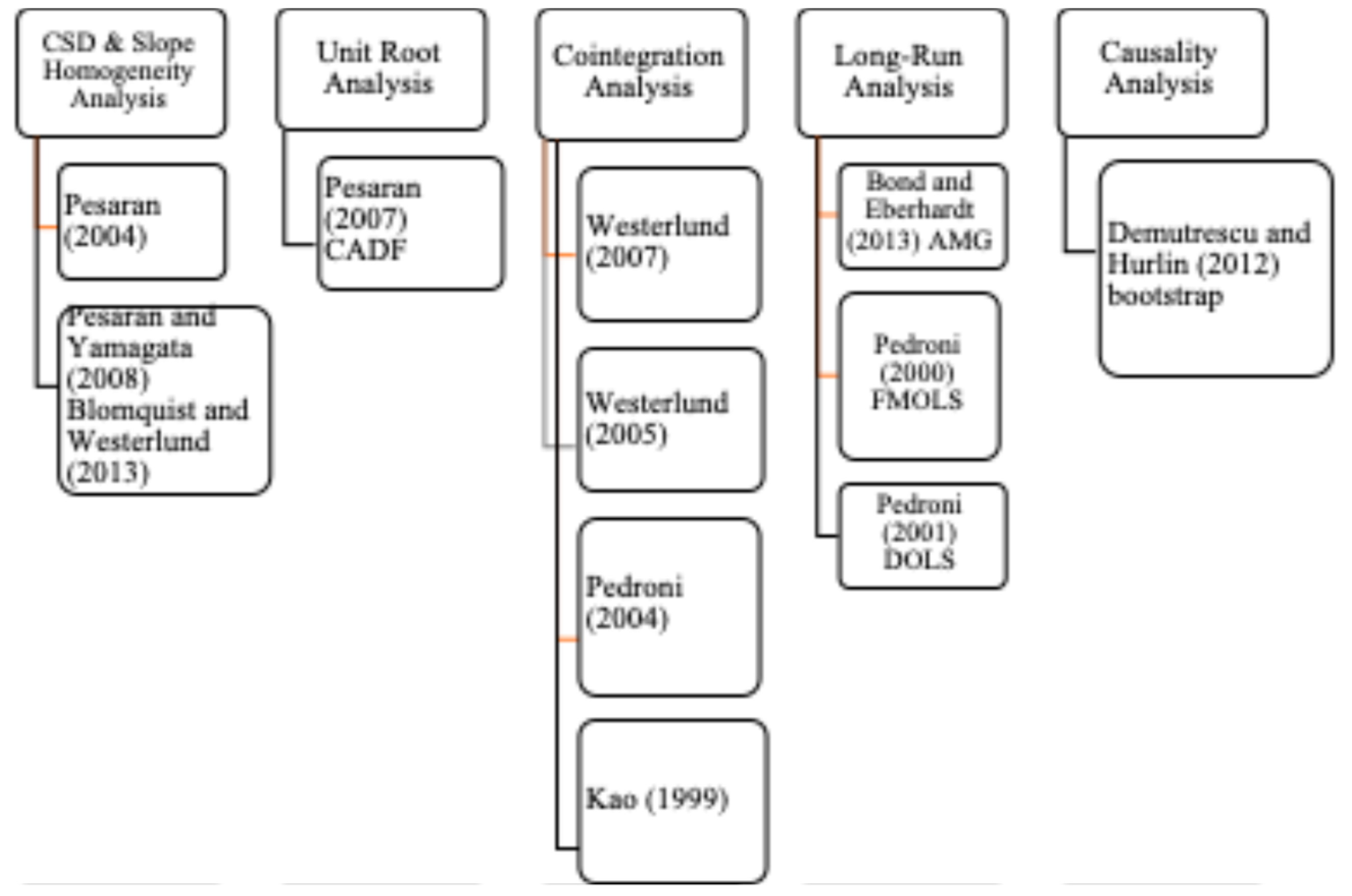

Table 1.
Description of variables.
| Variable | Symbol | Measurement | Source | Expected Sign |
|---|---|---|---|---|
| Ecological Footprint | EF | Global hectares per capita (gha) | GFN | - |
| Green Finance | GF | Renewable energy public R&D budget (% of total energy public R&D) |
OECD | (–) Feng et al. [36] |
| Green Growth | GGDP | CO₂ productivity (GDP per unit of energy-related CO₂ emissions) | OECD | (–) Chen et al. [66] |
| Economic Growth | GDP | Per capita GDP (2015 constant US$) | WDI | (+) Alola et al. [51] |
| Financial Globalization | FGL | Financial globalization index | Koff Swiss Institute | (+) Sadiq et al. [52] |
| Capital Formation | CAP | Gross capital formation (% of GDP) | WDI | (+) Khan & Hou [58] |
Table 2.
Descriptive statistics of the variables.
| lnEF | lnGF | lnGGDP | lnGDP | lnFGL | lnCAP | |
|---|---|---|---|---|---|---|
| Mean | 0.788 | 1.252 | 0.717 | 4.606 | 1.885 | 1.344 |
| Median | 0.771 | 1.294 | 0.716 | 4.611 | 1.906 | 1.345 |
| Std. dev. | 0.104 | 0.340 | 0.169 | 0.116 | 0.070 | 0.058 |
| Min. | 0.539 | -0.244 | 0.334 | 4.291 | 1.515 | 1.175 |
| Max. | 1.038 | 1.798 | 1.200 | 4.884 | 1.962 | 1.505 |
| Skewness | 0.387 | -1.195 | -0.043 | 0.201 | -2.148 | 0.062 |
| Kurtosis | 2.678 | 5.293 | 2.933 | 3.109 | 8.883 | 2.994 |
| Jarque-Bera | 10.304 | 160.567 | 0.175 | 2.542 | 776.151 | 0.228 |
| Prob. | 0.005 | 0.000 | 0.916 | 0.280 | 0.000 | 0.891 |
| Obs. | 351 | 351 | 351 | 351 | 351 | 351 |
Table 3.
Correlation matrix of model variables.
| Variables | lnEF | lnGF | lnGGDP | lnGDP | lnFGL | lnCAP |
|---|---|---|---|---|---|---|
| lnEF | 1.000 | |||||
| lnGF | 0.030 | 1.000 | ||||
| lnGGDP | 0.547 | 0.219 | 1.000 | |||
| lnGDP | 0.415 | 0.075 | 0.214 | 1.000 | ||
| lnFGL | 0.241 | 0.091 | 0.228 | 0.065 | 1.000 | |
| lnCAP | 0.058 | 0.122 | 0.057 | 0.082 | 0.108 | 1.000 |
Table 4.
Cross-Sectional Dependence (CD) test results.
| Variables | CD-test | p-value | Corr. | Abs(corr.) |
|---|---|---|---|---|
| lnEF | 28.64 | 0.000 | 0.624 | 0.625 |
| lnGF | 11.53 | 0.000 | 0.251 | 0.369 |
| lnGGDP | 37.81 | 0.000 | 0.824 | 0.824 |
| lnGDP | 39.71 | 0.000 | 0.865 | 0.865 |
| lnFGL | 32.61 | 0.000 | 0.711 | 0.714 |
| lnCAP | 7.19 | 0.000 | 0.157 | 0.400 |
Table 5.
Slope homogeneity test results.
| Title 1 | Test statistics | t-statistics | p-value |
|---|---|---|---|
| Pesaran and Yamagata (2008) | 12.724*** | 0.000 | |
| 14.784*** | 0.000 | ||
| Blomquist and Westerlund (2013) | 2.742*** | 0.006 | |
| 3.401*** | 0.001 |
Note: *** denotes significance at the 1% level.
Table 6.
Panel unit root test results.
| Variables | Constant | Constant and trend | |
|---|---|---|---|
| Level | lnEF | -1.717 | -2.638 |
| lnGF | -1.973 | -2.443 | |
| lnGGDP | -1.745 | -2.314 | |
| lnGDP | -1.629 | -2.496 | |
| lnFGL | -1.746 | -2.446 | |
| lnCAP | -1.612 | -1.945 | |
| First difference | lnEF | -2.902*** | -4.037*** |
| lnGF | -2.987*** | -3.817*** | |
| lnGGDP | -3.849*** | -3.827*** | |
| lnGDP | -2.602*** | -2.693* | |
| lnFGL | -3.260*** | -3.321*** | |
| lnCAP | -2.907*** | -3.168*** |
Note: *** denotes significance at the 1% level, and * denotes significance at the 10% level.
Table 7.
Cointegration tests results.
| Westerlund (2007) | Value | Z-value | p-value |
|---|---|---|---|
| Gt | -9.076*** | -24.324 | 0.000 |
| Ga | -1.201 | 6.025 | 1.000 |
| Pt | -15.393*** | -6.325 | 0.000 |
| Pa | -12.157 | -0.364 | 0.358 |
| Pedroni | Test statistic | p-value | |
| Modified Phillips-Perron t | 0.106 | 0.457 | |
| Phillips-Perron t | -8.311*** | 0.000 | |
| Augmented Dickey-Fuller t | -8.625*** | 0.000 | |
| Kao | Test statistic | p-value | |
| Modified Dickey-Fuller t | -5.614*** | 0.000 | |
| Dickey-Fuller t | -5.854*** | 0.000 | |
| Augmented Dickey-Fuller t | -0.220 | 0.413 | |
| Unadjusted modified Dickey-Fuller t | -13.518*** | 0.000 | |
| Unadjusted Dickey-Fuller t | -8.145*** | 0.000 | |
| Westerlund | Test statistic | p-value | |
| Variance Ratio | -1.668** | 0.047 |
Note: *** and ** denote significance at the 1% and 5% levels, respectively. The cointegration tests account for the cross-sectional dependence (CSD) structure.
Table 8.
AMG estimation results. Dependent variable: lnEF.
| Coefficient | Standard error | p-value | |
|---|---|---|---|
| lnGF | -0.023* | 0.013 | 0.073 |
| lnGGDP | -0.133* | 0.071 | 0.063 |
| lnGDP | 0.359*** | 0.088 | 0.000 |
| lnFGL | 0.237** | 0.114 | 0.039 |
| lnCAP | 0.202*** | 0.078 | 0.010 |
| Constant | -1.444*** | 0.347 | 0.000 |
| Wald χ2 | 34.00 | ||
| Prob. | 0.000 | ||
| RMSE | 0.014 | ||
| Obs. | 351 | ||
| Number of countries | 13 |
Note: *** denotes significance at the 1% level, ** at the 5% level, and * at the 10% level.
Table 9.
Robustness check: FMOLS and DOLS estimation results. Dependent variable: lnCO₂
| Variable | FMOLS Coefficient | p-value | DOLS Coefficient | p-value |
|---|---|---|---|---|
| lnGF | -0.726*** | 0.000 | -0.011*** | 0.000 |
| lnGGDP | -0.785*** | 0.000 | -0.594*** | 0.000 |
| lnGDP | 0.994*** | 0.000 | 0.690*** | 0.000 |
| lnFGL | 0.075** | 0.029 | 0.090 | 0.288 |
| lnCAP | 0.174*** | 0.000 | 0.343*** | 0.000 |
| Constant | ||||
| Obs. | 351 | 351 | ||
| No. of countries | 13 | 13 |
Note: *** denotes significance at the 1% level, ** at the 5% level.
Table 10.
Panel bootstrap causality test results. Dumitrescu–Hurlin Approach (Dependent variable: lnEF).
Table 10.
Panel bootstrap causality test results. Dumitrescu–Hurlin Approach (Dependent variable: lnEF).
| Null Hypothesis | W-stat. | Zbar-stat. | Bootstrap p-value | Results |
|---|---|---|---|---|
| lnGF ≠˃ lnEF | 2.438 | 3.666* | 0.055 | lnGF → lnEF |
| lnEF ≠˃ lnGF | 1.163 | 0.417 | 0.815 | No |
| lnGGDP ≠˃ lnEF | 4.869 | 9.866*** | 0.010 | lnGGDP ⇄ lnEF |
| lnEF ≠˃ lnGGDP | 3.620 | 6.681** | 0.015 | lnEF ⇄ lnGGDP |
| lnGDP ≠˃ lnEF | 4.652 | 9.312*** | 0.010 | nGDP → lnEF |
| lnEF ≠˃ lnGDP | 1.276 | 0.706 | 0.695 | No |
| lnFGL ≠˃ lnEF | 7.301 | 4.208* | 0.095 | lnFGL → lnEF |
| lnEF ≠˃ lnFGL | 4.796 | 1.015 | 0.640 | No |
| lnCAP ≠˃ lnEF | 2.673 | 4.266* | 0.060 | lnCAP → lnEF |
| lnEF ≠˃ lnCAP | 2.421 | 3.623 | 0.135 | No |
Note: ***, **, and * denote significance at the 1%, 5%, and 10% levels, respectively. Bootstrapped p-values are based on 500 replications. The optimal lag length was selected using the Schwarz Information Criterion (SIC).
Disclaimer/Publisher’s Note: The statements, opinions and data contained in all publications are solely those of the individual author(s) and contributor(s) and not of MDPI and/or the editor(s). MDPI and/or the editor(s) disclaim responsibility for any injury to people or property resulting from any ideas, methods, instructions or products referred to in the content. |
© 2025 by the authors. Licensee MDPI, Basel, Switzerland. This article is an open access article distributed under the terms and conditions of the Creative Commons Attribution (CC BY) license (http://creativecommons.org/licenses/by/4.0/).
Copyright: This open access article is published under a Creative Commons CC BY 4.0 license, which permit the free download, distribution, and reuse, provided that the author and preprint are cited in any reuse.


