Submitted:
16 April 2025
Posted:
17 April 2025
You are already at the latest version
Abstract
With the widespread application of facial image-based age estimation technologies in fields such as marketing, medical aesthetics, and intelligent surveillance, their importance has become increasingly evident. However, in real-world scenarios, facial images obtained are often incomplete due to occlusions caused by masks or sunglasses, which obscure the eyes, mouth, or nose to varying degrees. Such occlusions lead to the loss of critical facial feature information, thereby reducing the accuracy of age estimation. Although prior research has explored de-occlusion methods for occluded facial images, there remains a lack of studies focusing on the implicit facial feature information present in fixed occlusion patterns. To address this issue, this study proposes a novel method for reconstructing occluded facial features to enhance age estimation accuracy under occlusion conditions. This study introduces a facial feature reconstruction network based on knowledge distillation and feature reconstruction. The primary objective is to leverage complete facial information from a teacher model to guide a student network in fully extracting effective information from the unoccluded regions of occluded images. Additionally, the proposed method reconstructs feature maps of the occluded regions through a meticulous, layer-wise feature reconstruction process. The reconstructed network can then act as a feature encoder to provide more informative features for the age estimation regression module. Experimental results demonstrate that the proposed approach achieves superior performance in age estimation with randomly occluded images on the MORPH-2, AFAD, CACD and IMDB-WIKI datasets, with mean absolute errors (MAE) of 4.27, 4.83, 5.15 and 5.71, respectively. These results outperform existing occluded facial age estimation methods based on attention mechanisms and generative facial image reconstruction.
Keywords:
knowledge distillation
; facial feature reconstruction
; age estimation
; deep learning
1. Introduction
Facial feature learning plays an essential role in a variety of computer vision tasks, with age estimation gaining increasing relevance in fields such as statistical marketing analysis tailored to product preferences of specific age groups, the beauty and telemedicine industries, and age-based suspect identification in intelligent surveillance systems [1,2]. However, in practical applications, facial images often present significant challenges due to occlusions, which commonly disrupt the visibility of critical facial features [3]. Occlusion has been considered a highly challenging one. In real-life images or videos, facial occlusions can often be observed, e.g. facial accessories including sunglasses, scarves, and masks[4]. These occlusions not only obscure important facial information but also undermine the accuracy of age estimation. Given that facial features evolve with age—such as changes in skin thickness, texture, the sharpening of bone lines, and the development of wrinkles—these variations differ substantially between individuals [5], making automatic age estimation (AAE) [6,7,8] under occlusion conditions a particularly difficult problem. Despite considerable advancements in age estimation algorithms, data collection, system performance testing, and the establishment of rigorous evaluation protocols, improving the accuracy of age estimation continues to be a considerable challenge.
Age estimation typically involves three key stages: feature representation, feature extraction, and age prediction. Early approaches primarily relied on handcrafted feature extraction, which required domain-specific knowledge. However, the effectiveness of such knowledge is often difficult to verify and can limit the generalizability of the model. In contrast, convolutional neural networks (CNNs) offer the advantage of automatically extracting distinct and robust facial features, while also learning age-related information directly from the data [9]. In CNN-based age estimation, convolutional layers are responsible for extracting and encoding age-related features from facial images, while multi-layer perceptrons (MLPs) use these features to predict the subject’s age. A loss function measures the discrepancy between the predicted and true age, and backpropagation is employed to refine the model. This approach is fully automated and leverages features that are otherwise difficult to capture with prior knowledge. When compared to traditional techniques, CNN-based models have demonstrated superior performance in age estimation, and ongoing research continues to explore new methodologies to further improve their accuracy and effectiveness.
To tackle the challenges posed by occlusions, existing research has explored a variety of solutions, with a primary focus on local feature learning [10], attention mechanisms [11], and generative models [1,12]. Local feature learning methods partition the face into different regions and extract relevant features from the unoccluded areas, enabling age estimation even with partial occlusions. However, their performance degrades significantly when occlusion is more extensive. Attention mechanism-based techniques guide the model to concentrate on unoccluded regions while minimizing interference from occluded regions, though their effectiveness is strongly dependent on the size and shape of the occlusion. Generative models attempt to reconstruct complete facial information by inferring the unoccluded features. While these models can handle complex occlusions effectively, the generated regions often exhibit blurriness or distortion. Although these approaches have enhanced facial feature reconstruction under occlusion to some degree, they fail to fully exploit the relationships between occluded and unoccluded regions, which limits their accuracy in high-precision age estimation tasks. To address these limitations, this study proposes a novel approach combining knowledge distillation with layer-wise training for high-quality facial feature reconstruction under occlusion conditions. The approach utilizes a pre-trained age estimation model on unoccluded facial data as a teacher model and transfers its rich feature knowledge to a student model through knowledge distillation. During the layer-wise training and global fine-tuning process, the student model progressively learns to extract robust facial feature representations. Experimental results demonstrate that the proposed method significantly outperforms existing baseline models in both feature reconstruction quality and age estimation accuracy across various occlusion scenarios (Figure 1).
The key innovations of this study include:
- Novel Research Focus: This is the first study to address age estimation in the context of large-scale occlusions affecting the eyes and mouth regions.
- New Architecture: The proposed model introduces a knowledge distillation framework that facilitates the transfer of unoccluded facial feature knowledge from a teacher model to a student model without the need to compress model parameters.
- New Training Strategy: The training process integrates layer-wise feature reconstruction and parameter freezing to ensure accurate reconstruction of occluded facial features. Fine-tuning with original age labels is then performed to remove any noisy features.
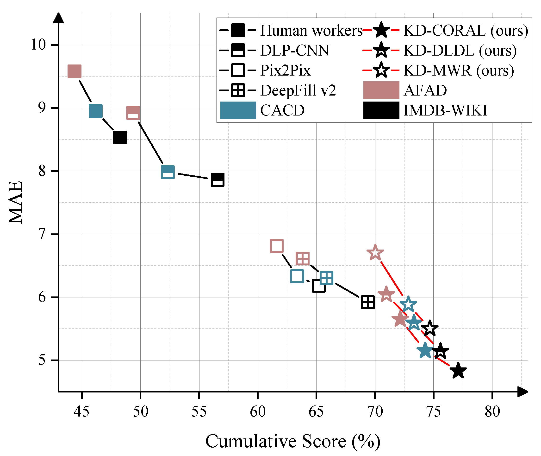
Figure 1.
In a comparison of various mainstream facial age estimation methods on the AFAD, CACD, and IMDB-WIKI datasets, our method achieved the best performance across multiple datasets. (Note: A higher Cumulative Score percentage indicates a lower age estimation error rate, and a smaller MAE indicates smaller age estimation errors.)
2. Related Works
Facial images contain a wide array of biological information, including ethnicity, gender, age, environment, and lifestyle characteristics. Buolamwini and Gebru (2018) analyzed the distribution and mean values of these attributes, proposing a method to assess biases in algorithms and databases [13]. This work has influenced numerous studies that make use of facial images [14,15,16].
2.1. Age Estimation
Traditional age estimation methods based on handcrafted features encounter several challenges, such as the necessity to account for various influencing factors and their reliance on expert knowledge, the accuracy of which is often unverifiable [17].
The rise of deep learning has led to the widespread adoption of convolutional neural networks (CNNs), which can automatically extract robust facial features and learn age-related information [9]. Since the introduction of deep learning, most age estimation methods have relied on CNNs. Age estimation methods are commonly categorized into four types [17]: (1) multi-class classification; (2) regression-based estimation; (3) deep label distribution learning (DLDL); (4) ranking-based learning. For example, a model called CNN2ELM was proposed in [18], which combines CNNs with extreme learning machines (ELMs) for age learning, achieving promising results in the ChaLearn 2016 competition. Another notable approach is the Deep Expectation of Apparent Age (DEX) system proposed in [19], which utilizes softmax expectation refinement based on the VGG-16 network. The DEX system treats age estimation as a classification problem, estimating age by multiplying age labels with the class probability distribution derived from the softmax output of the final VGG-16 layer. Although the DEX system performed well on large-scale datasets like IMDB-WIKI and MORPH-2, it did not account for the ordinal relationships between ages, limiting its ability to model age continuity.
Ranking-based methods improve performance by learning ordinal relationships among ages. For instance, OR-CNN [20] and Ranking-CNN [21] use multiple binary classifiers to determine whether the age of an input image exceeds a particular threshold, indirectly estimating age. These approaches better capture ordinal information but may not fully address the continuity of age. Deep Regression Forests (DRFs) [22] employ hierarchical decision trees to learn nonlinear features, achieving high accuracy in age estimation. However, regression-based methods often face performance degradation when data for certain age groups is sparse. Table 1 presents various age estimation methods under each category and their performance across different datasets.
To mitigate these limitations, Cao et al. [23] introduced a novel framework for ordinal regression tasks such as age estimation, ensuring classifier consistency and substantially enhancing prediction performance. Likewise, Gao et al. [24] addressed label ambiguity in age estimation by optimizing feature and classifier learning. Shin et al. [25] employed relative ranking (-rank) with local and global -regressors, coupled with iterative optimization, to achieve strong results in sequential regression tasks such as facial age estimation.

Table 1.
Summary of Age Estimation Methods
| Categories | Method | Database | MAE |
|---|---|---|---|
| Classification of multi-class ages | DEX [26] | IMDB-WIKI + LAP2015 | 3.22 |
| MORPH | 2.68 | ||
| FG-NET | 3.09 | ||
| CACD | 6.52 | ||
| Regression based on metrics | OR-CNN [20] | AFAD | 3.34 |
| MORPH | 3.27 | ||
| VGG + BridgeNet [27] | MORPH | 2.38 | |
| FG-NET | 2.56 | ||
| LAP2015 | 2.98 | ||
| Learning by the distribution of deep label | DLDL-v2 [28]] | LAP2015 | 3.14 |
| LAP2016 | 3.45 | ||
| MORPH | 1.97 | ||
| Ranking | Ranking-CNN [21] | MORPH | 2.96 |
2.2. Facial Occlusion in Age Estimation
Despite considerable advances in age estimation, several challenges persist in real-world applications. Facial images in practical scenarios are often impacted by issues such as low resolution, poor lighting, noise, and occlusions. Key facial regions like the eyes, nose, and mouth are particularly susceptible to occlusions, which result in the loss of crucial features and hinder the accuracy of age estimation. Although various studies [29,30,31,32] have explored occlusions caused by glasses, hats, scarves, and mobile devices, these approaches typically overlook the occluded areas, focusing instead on extracting features from the visible regions or attempting to generate the occluded regions from the unoccluded parts. However, these methods fail to fully utilize the relationships between occluded and visible facial features.
Current de-occlusion techniques mainly address partial occlusions. For example, the Attention-based Partial Face Recognition method [33] combines intermediate feature maps from ResNet with attention pooling and an independent aggregation module, allowing the model to focus on the unoccluded facial regions. However, in cases of extensive occlusions (e.g., when both the eyes and mouth are covered), the attention mechanism is less effective, leading to a significant drop in performance. Another method proposed by [34] integrates attention mechanisms within a residual network to highlight key facial regions, such as the unoccluded eyes, and utilizes a mask generator to detect and clean occluded features. However, the mask generator struggles to generalize well under complex occlusion conditions, limiting its practical utility.
Additionally, [29] introduced a two-stage occlusion-aware GAN based on the Pix2pix framework, which aims to remove occlusions by using randomly placed occlusion shapes. While the approach performs well in controlled scenarios, its applicability to more complex occlusions, such as those caused by the simultaneous occlusion of the eyes and mouth/nose, remains limited. Similarly, [35] uses a two-stage GAN to remove medical mask occlusions and reconstruct the occluded facial regions. While it demonstrates notable improvements, issues such as color consistency and detail accuracy in the reconstructed regions persist. Furthermore, some studies [32] employ labeled occluded images for supervised learning, adding extra channels to detect and remove occluded regions. However, these methods typically rely on large annotated datasets and struggle to handle cases with regions where both the eyes and the mouth/nose are simultaneously occluded.
2.3. Knowledge Distillation
Knowledge distillation [36] is a technique in which a teacher network instructs a student network by aligning the student’s predictions with the teacher’s predictions, while also incorporating the true labels. The teacher’s output is softened using a temperature parameter, which enhances the quality of supervision during training. The student network minimizes a loss function that combines traditional cross-entropy loss with a regularization term that encourages the student to learn from the teacher’s softened output.
To enhance performance, particularly in deep networks, FitNet [37] extends the concept of knowledge distillation by introducing intermediate layer guidance. This method aligns the intermediate features of both the teacher and student networks, facilitating the student’s ability to learn more expressive representations. In the pre-training phase, the student network is trained to match the teacher’s intermediate features. During the fine-tuning phase, the student further refines its output while ensuring consistency with both the teacher’s intermediate features and the true labels.
3. Proposed Methods
3.1. Overview of Suggested Method
The method proposed in this paper is based on the following prior facts: in the problem of facial occlusion, occluding objects (such as sunglasses, masks, veils, etc.) typically cover specific regions of the face, primarily the eyes and mouth, and the positions and types of these occluding objects are usually fixed. As a result, there is a certain regularity between the occluded areas and the position of the occluding object. When humans see an image of a face with some occlusion, even if part of the face is occluded, we can still infer or imagine the complete facial image based on the visible (non-occluded) parts and estimate the apparent age of the person in the image. This indicates that although the eyes and mouth may be occluded, the human brain can reasonably infer the features of the occluded parts by observing the non-occluded parts. Furthermore, under the premise that the occluding object covers fixed positions, there is an implicit mapping relationship between the features of the occluded and non-occluded parts. Even if some parts are occluded, as long as the features of the non-occluded parts are known, the features of the occluded parts can be inferred. For example, based on the forehead, chin, and facial contours, the features of occluded parts like the eyes and mouth can still be predicted. In traditional methods, the occluded parts are often ignored, and only the non-occluded parts of the face (such as the non-occluded facial region) are considered. Ignoring the important visual information of the occluded parts leads to the loss of crucial details in the image. Moreover, past methods have over-relied on age labels during the training process, while there is a lack of sufficiently annotated facial datasets with age labels, and obtaining such data is both expensive and time-consuming. More importantly, existing datasets often do not account for the various occlusion scenarios that are commonly found in the real world (such as masks, glasses, veils, etc.), which causes models trained on these datasets to be unable to handle various facial occlusion problems in real-world scenarios. Based on these considerations, this study proposes a novel, integrated framework that optimizes the reconstruction of facial features under occlusion conditions specifically for age estimation tasks, using knowledge distillation and a layer-by-layer training strategy. The core of this framework lies in utilizing the rich feature representations in a pre-trained teacher model to guide the student model in learning the mapping relationship between occluded and non-occluded features across different dimensions, thereby reconstructing high-quality facial features. The layer-by-layer training strategy allows the model to gradually transition from learning simple low-level features (such as edges and textures) to more complex high-level features (such as facial contours and details), enhancing the model’s ability to recover information in complex scenarios. To reduce over-reliance on age labels, this method employs a self-supervised training approach during the layer-by-layer knowledge distillation process, adding various occlusions to the facial images and using the original image itself as the supervisory signal for training the model. This means that during training, the model does not need to rely on external age labels. Age labels are only used in the final global fine-tuning phase to eliminate the noise effects caused by occlusion.
Three robust age estimation models—CORAL, DLDL, and MWR—are chosen as teacher models based on their complementary strengths: CORAL utilizes ordinal regression to capture age relationships, DLDL incorporates label distribution learning to account for age uncertainty, and MWR predicts both the mean and variance of age to provide confidence intervals. To ensure consistency between intermediate feature maps, the student model shares the same encoder architecture as the teacher models, eliminating the need for model compression.
During the training process, feature reconstruction starts at shallow layers and progressively advances to deeper layers. The intermediate feature maps of the teacher models serve as supervisory signals, with an L2 loss function applied to minimize the discrepancies between student and teacher features. Once a layer’s reconstruction is complete, its parameters are frozen, thereby enforcing hierarchical learning from low-level textures to high-level semantic features. After the layer-wise training phase, all parameters of the student model are unfrozen and globally fine-tuned using the original age labels. This final step removes residual noise introduced during the distillation process and ensures the alignment of reconstructed features with the ground-truth characteristics. As detailed in Algorithm 1, the process involves layer-wise distillation with feature alignment and subsequent fine-tuning.
| Algorithm 1 Layer-wise Distillation with Feature Alignment and Fine-tuning |
|
As shown in Figure 2, during inference, a binary classification convolutional neural network is deployed to detect occlusions (e.g., sunglasses or masks). If occlusion is detected, the input is routed to the student model for feature reconstruction; otherwise, it is directly processed by the teacher model. The final features from either model are then fed into the age estimation module for prediction.
3.2. Feature Alignment
This study introduces a feature reconstruction module based on knowledge distillation, which facilitates the completion and alignment of occluded region features through a teacher-student model framework. The teacher model extracts features from full-face images, while the student model operates on occluded face images. After each residual block, the feature maps of the teacher model guide the reconstruction of the student model’s feature maps.
Let the input features of the full-face image and the occluded face image be represented as and , respectively. Both the teacher and student models adopt the ResNet-34 architecture. The teacher model extracts global features from complete, unoccluded images, while the student model extracts partial features from occluded images. After each residual block, the feature map from the teacher model is aligned with the corresponding feature map from the student model .
At each residual block l, a feature alignment module aligns the student model’s feature map with the teacher model’s feature map. The aligned features are then passed as inputs to the next network layer, allowing the student model to capture the complementary relationship between the occluded and unoccluded regions. The feature alignment process is computed as follows:
where Conv represents the convolution operation, and Concat denotes the concatenation of feature maps along the channel dimension. By fusing feature information from both the teacher and student models, the aligned feature map enables the student model to learn the implicit relationships between occluded and unoccluded regions, thereby facilitating the reconstruction of occluded features.
3.3. Feature Distillation Mechanism
To further refine the feature reconstruction process, this study introduces a feature distillation mechanism. After each residual block, the loss between the feature maps of the teacher and student models is computed to regularize the student model’s learning process:
where denotes the dimensions of the feature map at layer l. Minimizing the feature distillation loss allows the student model to learn more effectively from the teacher model’s feature representations, thereby enhancing the reconstruction accuracy of the occluded regions.
3.4. Layer-Wise Reconstruction and Global Fine-Tuning
After completing feature distillation for each layer, the parameters of the current layer are frozen to ensure that the training of subsequent layers does not interfere with the already reconstructed features. The process then continues with the feature distillation for the next layer until the feature maps of all layers have been reconstructed.
Once feature distillation is completed for all residual blocks, all layers’ parameters are unfrozen, and global fine-tuning is performed using the original age labels. The loss function during fine-tuning remains consistent with the original age regression module’s loss function, further optimizing the model’s feature representations and improving age estimation accuracy.
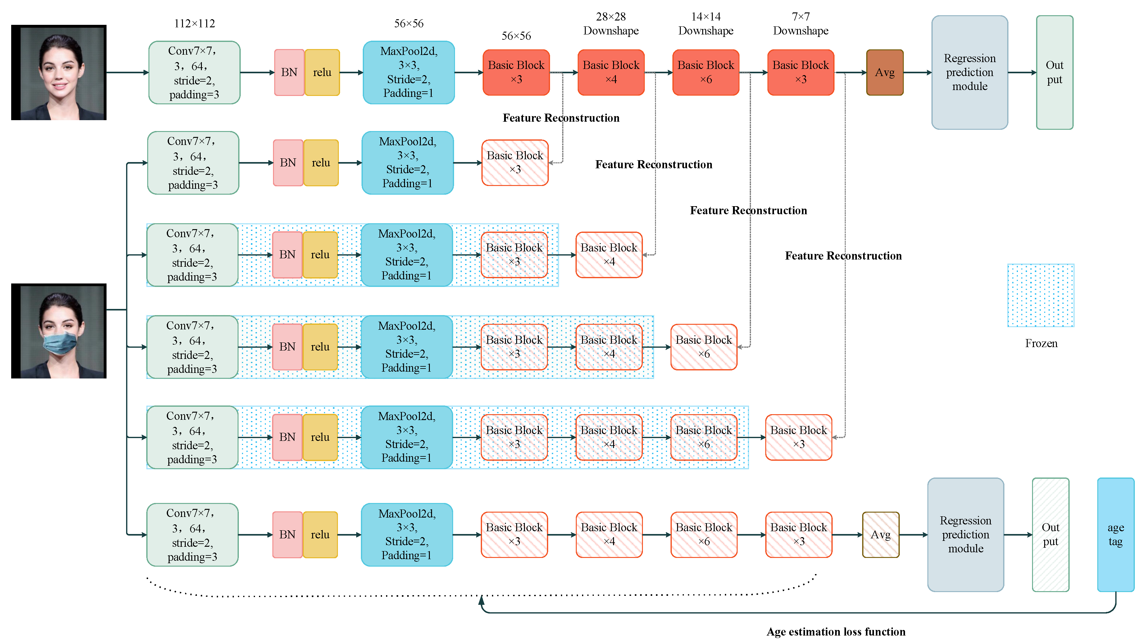
Figure 3.
Using ResNet-34 as the feature extraction network, the student’s feature maps after each residual block are trained to match those of the teacher network. Features are extracted from an occluded dataset, where the teacher network’s feature maps serve as a supervisory signal, guiding the student’s feature reconstruction layer by layer. After reconstructing the feature map at each residual block, all previous network layers are frozen before proceeding to the next layer’s training. In the fine-tuning stage, all network layers are unfrozen and fine-tuned using real age labels to remove residual noise features.
4. Experimental Results
This study evaluates the performance of the proposed method for facial age estimation under various occlusion conditions through a series of experiments. The primary focus was on assessing the baseline model’s performance under occlusion, investigating the impact of knowledge distillation strategies on the student model, analyzing the enhancement of model performance through layer-wise training, and exploring the contribution of global fine-tuning to further optimize the model. Additionally, the proposed method is compared with other advanced models for occluded facial age estimation. The following sections detail the datasets, experimental setup, results, and corresponding analysis.
4.1. Dataset and Experimental Setup
In this section, we describe the dataset creation, preprocessing, and the configuration of the experimental setup. To evaluate the influence of various methods on facial age estimation under occlusion, a dedicated dataset featuring multiple types and degrees of occlusion was created. The dataset creation process is outlined as follows: four publicly available foundational datasets containing rich facial image data were selected: CACD [38], AFAD [20], MORPH-2 [39], and IMDB-WIKI [40].
The MORPH-2 dataset consists of 55,608 facial images and can be accessed at https://www.faceaginggroup.com/morph/. Age labels in this dataset range from 16 to 70 years. It is a widely used dataset for age estimation tasks due to its extensive number of images and diversity in age, ethnicity, and gender. For our experiments, we split the dataset into two independent subsets: 80% for training and 20% for testing.
The CACD dataset (Chen et al., 2014), available at http://bcsiriuschen.github.io/CARC/, contains 159,449 images with ages ranging from 14 to 62 years. Similar to the MORPH-2 dataset, the faces in the CACD dataset are centered, with the tip of the nose aligned to the center. This dataset offers a broad spectrum of images, making it ideal for evaluating age estimation models.
The AFAD dataset (Niu et al., 2016) contains 165,501 images of Asian faces, with ages ranging from 15 to 40 years, and can be downloaded from https://github.com/afad-dataset/tarball. Since the faces in this dataset are already centered, no further alignment was necessary. The AFAD dataset is particularly useful for testing age estimation models on younger age groups, providing an additional important subset for evaluation.
The IMDB-WIKI dataset, which includes over 500,000 facial images with age labels ranging from 0 to 100 years, covers a wide range of ethnicities, age groups, and facial expressions. It is divided into two parts: IMDB (460,723 images) and WIKI (62,328 images), and can be accessed at https://data.vision.ee.ethz.ch/cvl/rrothe/imdb-wiki/.
For preprocessing, we used MTCNN (Multi-task Cascaded Convolutional Networks) [41] for facial landmark detection. The images were then cropped to center the faces and standardize their sizes. This preprocessing step ensures that the faces are aligned and their appearances remain consistent across different datasets. All models were trained on the MORPH-2 dataset, which contains a diverse range of facial images spanning multiple age groups. The remaining datasets (AFAD, CACD, IMDB-WIKI) were used to assess the model’s performance across datasets.
All experiments were conducted under the same hardware and software conditions to ensure comparability and fairness. Specifically, we used an NVIDIA 3080 GPU for computation, and PyTorch was employed as the deep learning framework. In all experiments, the training process for all models followed identical hyperparameter settings, including the learning rate, optimizer, and the number of training epochs.
To comprehensively assess the impact of occlusion on face age estimation, we designed six different types of occlusion conditions: occlusion of the eye region using various types of sunglasses, blacking out the eye region, occlusion of the mouth region using different types of masks (including veils), blacking out the mouth region, simultaneous occlusion of both the eyes and mouth with glasses and masks, and simultaneous blacking out of both the eye and mouth regions with black blocks.These occlusion methods cover common facial obstructions in the real world. In real life, facial photos often lose parts of the image due to sunglasses and masks, while the application of black blocks can directly test the impact of occlusion on model performance without introducing noise variables.To ensure the accuracy of model performance analysis by minimizing the impact of the quantified occlusion area, we control the size of the mask and mouth blocks to cover 30%-35% of the facial image area, and the size of the sunglasses and eye blocks to cover 15%-20% of the facial image area during the occlusion process. All images are uniformly resized to 256×256×3. During the training phase, images are randomly cropped to 224×224×3 to meet the input requirements of ResNet-34, with data augmentation applied. In the model evaluation phase, the center of the 256×256×3 image is cropped to 224×224×3 as the model input.ensuring a fair comparison.The MORPH-2 dataset is randomly split into 80% for training and 20% for testing, with all models being trained on the MORPH-2 dataset., and the dataset division is shown in Table 2.
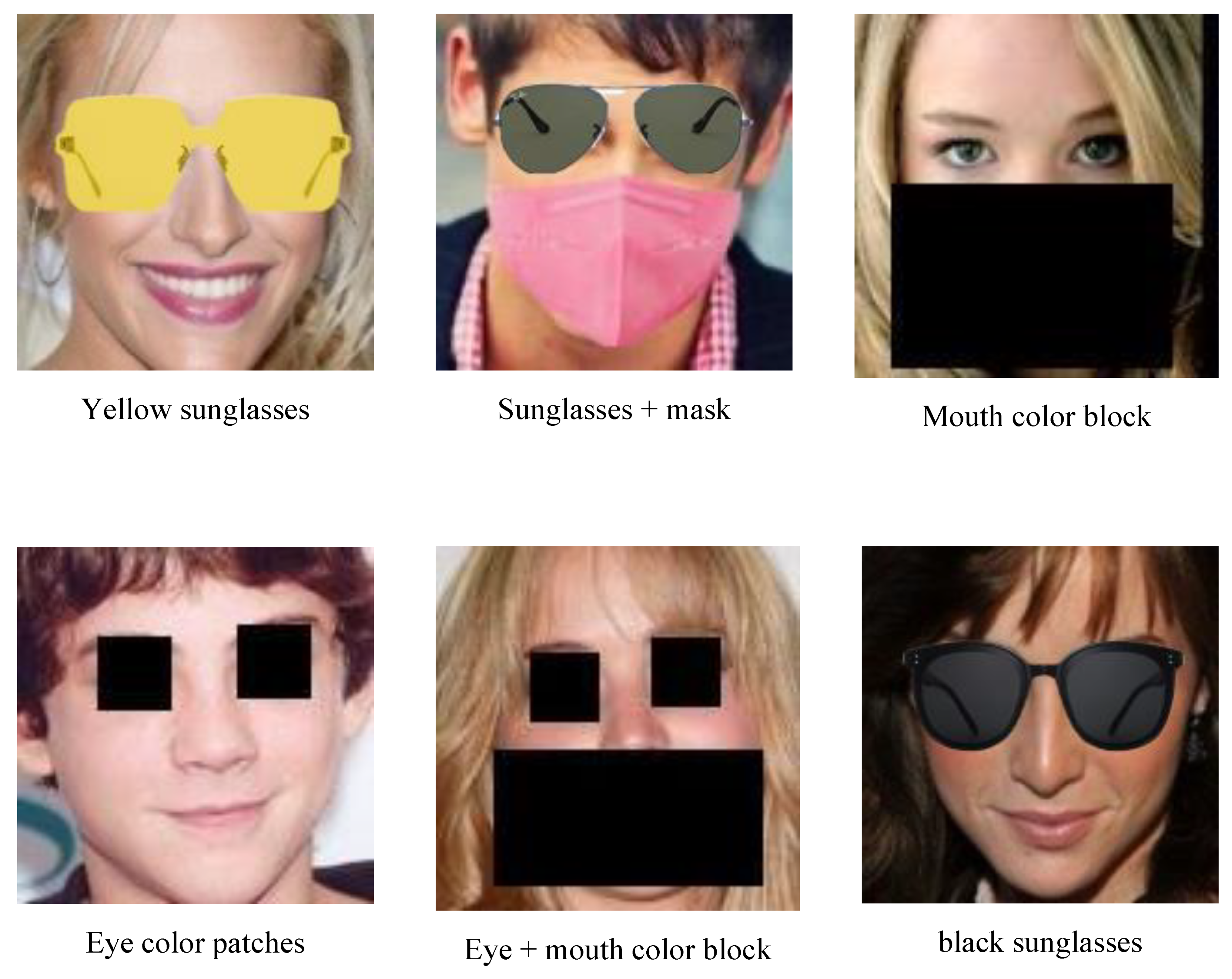
Figure 4.
Examples of partially occluded images are shown. In the actual experiments, 10 different types of sunglasses and 10 types of face masks were used.
Figure 4.
Examples of partially occluded images are shown. In the actual experiments, 10 different types of sunglasses and 10 types of face masks were used.
4.2. Performance Verification Experiment
4.2.1. Neural Network Architectures
In the model design of this paper, we first use an age estimation network pre-trained on an unoccluded dataset as the teacher model to guide the student model’s learning. The teacher model selects three models that perform well in the age estimation task: CORAL, DLDL, and MWR:
The CORAL (Cumulative Ordinal Regression) model effectively utilizes the ordinal relationship of age labels by converting the age estimation task into multiple sequential binary classification problems. This model divides the age labels into binary classification tasks, where the k-th binary task determines whether the sample’s age reaches or exceeds the threshold . For example, for K age levels, CORAL contains binary classifiers, each sharing the same weight parameters but with independent bias terms, ensuring consistency and monotonicity of the predictions. The loss function for CORAL is defined as:
where is the true label of sample i in the k-th binary classification task, indicating whether the sample’s age reaches the threshold , and is the probability predicted by the model for sample i in the k-th task, calculated by the Sigmoid function:
where is the output of the shared weight layer, and is the bias for the k-th task. To ensure ordering consistency, the CORAL model requires:
ensuring that the predicted probabilities for each task satisfy monotonicity:
DLDL (Deep Label Distribution Learning) transforms the age estimation task into label distribution learning by constructing the probability distribution of age labels to capture the uncertainty of age. The output layer of DLDL contains the probability for each age label, representing the probability distribution over ages. By predicting a probability distribution instead of a single age value, DLDL reflects the ambiguity in age estimation, leading to higher robustness when processing real-world data, especially when age labels are vague or hard to annotate accurately. The label distribution is modeled using a Gaussian distribution, with the distribution center at the true age and standard deviation , defined as follows:
where
The optimization goal of DLDL is to minimize the Kullback-Leibler (KL) divergence between the predicted age distribution and the true label distribution y, so that the predicted distribution is as close as possible to the true label distribution:
where is the true label distribution probability at age label k, and is the predicted probability by the model. By learning the probability distributions between different ages, DLDL better captures the ambiguity of age, thus improving robustness in the presence of sparse data or imprecise labels.
MWR (Moving Window Regression) is an innovative ordinal regression algorithm that achieves precise estimation of ordered data by predicting relative ranks (-rank). Traditional ordinal regression typically predicts the absolute value of the target, whereas MWR uses the concept of -rank, transforming the prediction task into estimating the relative position with respect to reference points. The definition of -rank is as follows:
where is the absolute rank of the input instance x, is the mean rank of reference points and , and is half the difference in their ranks. By predicting the -rank, the model can reconstruct the absolute rank of the input using the following formula:
The MWR algorithm first selects several reference points using a nearest-neighbor approach and calculates their average rank as the initial estimate. Then, using this initial estimate as the center, it forms a search window by iteratively selecting two reference points, optimizing the -rank, and progressively approaching the target value. In the t-th iteration, the update rule is:
where is the predicted -rank in the t-th iteration, and is the window size. This optimization process continues until the predicted value converges or the maximum number of iterations is reached.
The loss function for MWR is defined as the squared error of the -rank:
where is the predicted -rank by the model, and is the true value.
4.2.2. Implementation Details
The architectures of the three age estimation models consist of an encoder and a regression prediction module. To avoid introducing empirical bias by designing our own CNN architecture for comparing ordinal regression methods, we unify the encoders of all three models as the standard architecture ResNet-34[42] and retain the original regression module structure and loss function to train the teacher network. During training, we use a batch size of 128, train for 50 epochs, and optimize with the Adam optimizer, with an initial learning rate of , which is gradually reduced based on the validation set performance. In the backpropagation process, we freeze the feature extraction network parameters for the first 20 epochs, optimizing only the output layer for the age estimation task; after 20 epochs, we unfreeze the feature extraction network parameters and globally optimize the entire network, allowing the model to learn features useful for the output layer’s age estimation, with the best model selected based on MAE performance on the validation set.
In the training of the student model, the student model extracts features from a dataset with occlusions, while the feature maps from each layer of the teacher model are used as supervisory signals to guide the student model in optimizing the same layer of the network. Since the core task of this study is to reconstruct the features of occluded images rather than model compression, we maintain the structural consistency between the student and teacher networks during training. The training process follows a layer-wise learning approach: first, the parameters of the student model’s current layer are frozen, and the next layer is gradually learned until all hidden layers’ features are reconstructed. Initially, only the student model’s bottom feature layer (layer1) is unfrozen, with the remaining three residual blocks frozen. L2 loss is used to bring the student model’s low-level feature map closer to that of the teacher model, trained for 40 epochs with a learning rate of . Next, the second feature layer (layer2) is unfrozen, while the others remain frozen, and L2 loss is used to optimize feature differences, trained for 40 epochs with a learning rate of . Then, the middle (layer3) and high layers (layer4) are sequentially unfrozen, each trained for 40 epochs, continuing to optimize feature differences with L2 loss, with the learning rate gradually reduced to and . Through this sequential unfreezing and training approach, the student model can approximate the teacher model’s feature expression in a layer-wise learning process, starting with simple low-level features and gradually building up to complex high-level features, ultimately achieving high-quality feature reconstruction.
However, features reconstructed through this method may still retain some meaningless or even harmful noisy features. Therefore, the final step of training involves unfreezing all network layers and performing global fine-tuning for 50 epochs using the original age labels to further eliminate noisy features and retain valuable ones. During the global fine-tuning process, the loss function should remain consistent with the teacher model’s loss function during pre-training to ensure the student model learns the teacher model’s feature expression to the greatest extent.
4.2.3. Ablation Study
As presented in Equation (1), we employed the mean absolute error (MAE), which is the most commonly used metric[43,44], to assess the accuracy of age estimation. A lower MAE value indicates a higher accuracy in age estimation performance. where N is the total number of samples, represents the actual age, and denotes the predicted age. A lower MAE value indicates better performance in age estimation.
The MAE values for the CORAL, DLDL, and MWR models, when directly tested on the unoccluded dataset, were 3.12, 3.23, and 3.39, respectively. However, upon testing on a dataset with 50% randomly occluded images, the MAE values increased to 5.62, 5.82, and 5.89, respectively. While all three models exhibited strong performance on the unoccluded dataset, the tests on the dataset with random occlusions revealed a substantial increase in the MAE for all models, indicating that facial occlusion significantly impairs the models’ ability to estimate age accurately. Figure 5 visually illustrates the extent of the effect of random occlusion on model performance.
In order to analyze the specific impact of different occlusion methods on model accuracy, we evaluated the performance of the three pre-trained baseline models under various occlusion conditions. The results demonstrated that the MAE values of the CORAL, DLDL, and MWR models, under different occlusion scenarios, reflect the varying effects of different occlusion types on model performance. For single occlusions, the MAE values when wearing a mask were 5.51 (CORAL), 5.72 (DLDL), and 6.44 (MWR); and when wearing sunglasses, the MAE values were 6.21 (CORAL), 6.44 (DLDL), and 6.32 (MWR). When both a mask and sunglasses were simultaneously worn, the MAE values increased to 7.52 (CORAL), 7.71 (DLDL), and 7.82 (MWR). It was observed that occlusion of the eyes had a more pronounced impact on model performance compared to the occlusion of the mouth and nose. When both types of occlusion were present, the performance of the models declined markedly. Figure 6 presents the impact of various occlusion methods on model performance. Furthermore, we examined the effect of using color blocks as a direct occlusion technique instead of physical occlusion objects. The experimental results indicated that the use of color block occlusion also led to a reduction in model accuracy, although the impact was slightly less severe compared to using physical occlusion objects. Our analysis suggests that the color block occlusion method introduces less complexity, whereas the use of diverse physical occlusion objects, with varying colors, textures, and shapes, introduces greater uncertainty, thereby introducing more complex noise to the model. Table 3 provides a comparison of the impact of all occlusion methods on model performance.
To validate the impact of layer-wise feature reconstruction on the performance of age estimation models, we tested the MAE values of three baseline models on the MORPH-2 dataset with 100% random occlusion. The experimental results show that after layer-wise feature reconstruction, all three models achieved varying degrees of MAE reduction. This demonstrates that reconstructing occluded features provides age estimation models with more informative facial features, thereby effectively improving the accuracy of age estimation. Table 4 shows the effect of feature reconstruction on model accuracy.
To further validate the impact of using original age labels on the accuracy of age estimation models, we compared the accuracy of three baseline models after layer-wise feature reconstruction, both before and after fine-tuning with age labels. Table 5 presents the MAE values of the models after global fine-tuning. The results indicate that all three models achieved further accuracy improvements, demonstrating that fine-grained tuning better adapts to the age distribution within the dataset, enabling the models to provide more accurate estimations across different age groups.
Table 4.
MAE of the models with and without layer-wise feature reconstruction on the MORPH-2 dataset with random occlusion.
Table 4.
MAE of the models with and without layer-wise feature reconstruction on the MORPH-2 dataset with random occlusion.
| Model | MAE | |
|---|---|---|
| Baseline | Layer-wise Feature Reconstruction | |
| CORAL | 6.62 | 4.59 ↓ 2.03 |
| DLDL | 6.88 | 4.91 ↓ 1.97 |
| MWR | 6.85 | 5.08 ↓ 1.77 |
Note: Lower MAE values indicate higher accuracy in age estimation. The red arrows show the reduction in MAE after layer-wise feature reconstruction.
Although feature reconstruction enhances the model’s capability, it still retains some noisy features. By incorporating age labels for global fine-tuning, the models effectively eliminate these noise features, resulting in more precise final estimations. Therefore, the fine-tuning process not only improves model performance but also significantly enhances the model’s adaptability to complex data characteristics, thereby boosting overall model accuracy.
Table 5.
MAE of the models before and after global fine-tuning with original age labels.
| Model | MAE | |
|---|---|---|
| Layer-wise Feature Reconstruction | Layer-wise Feature Reconstruction + Age Label Fine-tuning | |
| CORAL | 4.59 | 4.27 ↓ 0.32 |
| DLDL | 4.91 | 4.43 ↓ 0.48 |
| MWR | 5.08 | 4.87 ↓ 0.21 |
Note: Lower MAE values indicate higher accuracy in age estimation. The red arrows show the reduction in MAE after fine-tuning with age labels.
4.2.4. Comparison Experiment
To test the impact of different backbone networks on model performance, we tested six backbone networks: ResNet-34, ResNet-50, ResNet-101, VGG16[45], EfficientNet-B0 [46], and InceptionV4 [47], evaluating their performance after layer-wise feature reconstruction and age label fine-tuning, as shown in Table 6. EfficientNet employs a compound scaling method. By simultaneously adjusting the network’s width, depth, and resolution, it balances model accuracy and computational efficiency. The design goal of EfficientNet is to achieve more efficient utilization of parameters and computational resources, so it generally delivers better performance with lower computational resources compared to the ResNet series architectures. However, when computational resources are abundant, ResNet networks can achieve better performance as the network depth increases. Although VGG16 performs well in traditional classification tasks, age estimation is a regression task rather than a simple classification task. Its relatively simple structure may not be sufficient to capture the complex features needed, and the excessive number of fully connected layers makes the VGG16 network parameter-heavy, resulting in lower computational efficiency and requiring more computational resources during training. Figure 7 visually demonstrates the impact of different backbone networks on the performance of the age estimation task.
To fully demonstrate the effectiveness of the layer-by-layer distillation approach, we directly trained and fine-tuned three baseline models on the MORPH-2 dataset with multiple occlusion types. The occlusion types in the dataset are shown in Table 7, and we compare the experimental results with those of our student model.
The results in Table 8 show that the layer-wise feature reconstruction combined with fine-tuning significantly outperforms the baseline model trained directly on the occluded dataset. This is because the model trained directly on the occluded dataset relies solely on visible features, failing to fully exploit the relationship between the occluded and unoccluded regions, which results in suboptimal feature representations. Additionally, the model learns a substantial amount of noise features introduced by occlusions, further degrading its performance. In contrast, layer-wise feature reconstruction allows the model to progressively reconstruct features from low-level to high-level, ensuring that it can learn more informative and accurate facial features while gradually mitigating the impact of noise features.
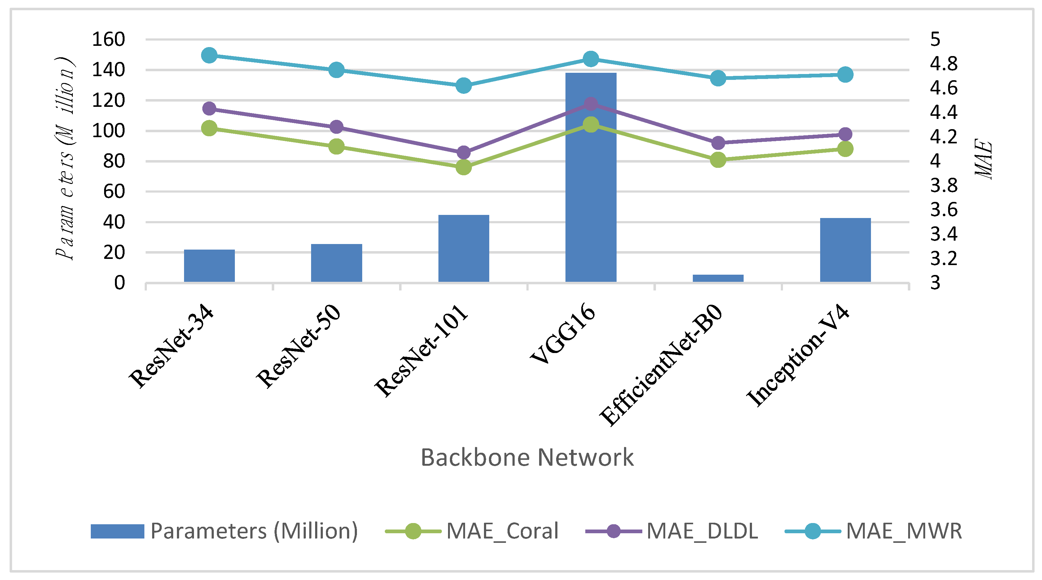
Table 6.
Comparison of Models with Parameters, Layers, and MAE under different regression methods.
| Model | Parameters (Millions) | Layers | MAE | ||
|---|---|---|---|---|---|
| CORAL | DLDL | MWR | |||
| ResNet-34 | 21.8 | 34 | 4.27 | 4.43 | 4.87 |
| ResNet-50 | 25.6 | 50 | 4.12 | 4.28 | 4.75 |
| ResNet-101 | 44.5 | 101 | 3.95 | 4.07 | 4.62 |
| VGG16[45] | 138.0 | 16 | 4.30 | 4.47 | 4.84 |
| EfficientNet-B0 [46] | 5.3 | 237 | 4.01 | 4.15 | 4.68 |
| InceptionV4 [47] | 42.5 | 48 | 4.10 | 4.22 | 4.71 |
Figure 7.
Performance comparison of six backbone networks—ResNet-34, ResNet-50, ResNet-101, VGG16, EfficientNet-B0, and InceptionV4—on three age estimation tasks: CORAL, DLDL, and MWR.
Figure 7.
Performance comparison of six backbone networks—ResNet-34, ResNet-50, ResNet-101, VGG16, EfficientNet-B0, and InceptionV4—on three age estimation tasks: CORAL, DLDL, and MWR.
Table 7.
Proportion of Six Occlusion Types in the MORPH-2 Dataset
| Occlusion Type | Proportion (%) |
|---|---|
| Mask | 15% |
| Sunglasses | 15% |
| Mask + Sunglasses | 20% |
| Mouth Color Block | 15% |
| Eyes Color Block | 15% |
| Mouth + Eyes Color Block | 20% |
4.2.5. Cross-Dataset Comparison with Multiple Advanced Models
To ensure the model can correctly route the images, we trained a binary classification convolutional neural network for occlusion detection. The model’s class labels were set to “face” and “occluded_face” to allow the model to effectively distinguish between faces with and without occlusions. In the network architecture, the input layer accepts color face images of size 224x224 pixels. Features are then extracted through multiple convolutional and pooling layers, followed by a global average pooling layer that converts the feature map into a one-dimensional vector. The output layer contains two neurons, using the Sigmoid activation function to output the probability for each class.
During training, binary cross-entropy was used as the loss function to optimize the model’s ability to distinguish between the two classes. The optimizer was Adam with an initial learning rate of 0.001, a training batch size of 32, and 50 epochs. To enhance the model’s generalization ability, we applied various data augmentations, including random rotations, flips, and color jittering. The performance on the validation set was monitored during training, and an early stopping strategy was applied to prevent overfitting. In this way, the trained detector was able to accurately identify whether the face region in the input image had occlusion, achieving good classification results.
To validate the cross-dataset performance of the model, we conducted random occlusion tests on the AFAD, CACD, and IMDB-WIKI datasets, comparing the results with several mainstream occluded face age estimation models. A group of human workers, who manually estimated ages from occluded facial images, served as the baseline for the age regression task. We compared the performance of human workers, DLP-CNN [48], Pix2Pix [49], DeepFill v2 [50], LCA-GAN [1], MCGRL[6], and our methods (using CORAL, DLDL, and MWR as the underlying models) for occlusion-aware facial age estimation in terms of MAE and CS(%).All comparison models were retrained on the MORPH-2 dataset, with the occlusion types divided according to Table 7, ensuring consistency in the training conditions.For all methods, we performed tests on different datasets where the test set randomly applied various mixed occlusions to 50% of the facial images, while the other 50% remained unchanged.
Table 9 shows that the KD-CORAL model, using CORAL as the age regressor, achieves the best performance in our experiments across multiple datasets. Additionally, we observed significant differences in MAE and CS performance among the various models across the three datasets. For all methods, the overall performance on different datasets follows the order: AFAD > CACD > IMDB-WIKI. We attribute this to the fact that the CACD dataset includes some low-quality images (e.g., 20×20 pixels) and has a wide age range (14-62 years), requiring the model to consider a broader age span. The IMDB-WIKI dataset, on the other hand, uses an automated labeling process, resulting in lower annotation quality and significant label noise. We found many photos where the apparent age did not match the labeled age, and some images even lacked faces. Additionally, there is a data imbalance issue, with a severe lack of images in younger age groups. As a result, the model performance showed a noticeable decline when tested on this dataset.Due to LCA-GAN employing a more complex attention mechanism for pixel-level de-occlusion reconstruction, it exhibited the best performance on the high-quality AFAD dataset. However, its performance showed significant degradation on the lower-quality CACD and IMDB-WIKI datasets. Experimental results show that our method still performs well under lower image quality, as the layer-by-layer detailed feature reconstruction allows the model to focus on different feature dimensions of the image, which maximizes the model’s robustness.
5. Conclusions
This paper proposes a knowledge distillation-based framework for facial feature reconstruction, effectively recovering critical features lost due to occlusion. Experimental results show that the method significantly enhances the robustness of age estimation models under various occlusion conditions. Future work will focus on reducing data biases, handling more complex occlusion patterns, and extending the framework to tasks such as facial expression recognition and pose estimation. Additionally, developing a more representative occlusion dataset will be key to improving practical applications.
Author Contributions
Conceptualization, Qilu Zhao; methodology, Qilu Zhao; software, Qilu Zhao and Shuangfei Yu; formal analysis, Qilu Zhao and Shuangfei Yu; investigation, Qilu Zhao; resources, Qilu Zhao; data curation, Shuangfei Yu; visualization, Qilu Zhao; writing—original draft preparation, Shuangfei Yu; writing—review and editing, Qilu Zhao. All authors have read and agreed to the published version of the manuscript.
Funding
This work was supported by the Shandong Provincial Natural Science Foundation, China (No. ZR2023MF106).
References
- Nam, S.H.; Kim, Y.H.; Choi, J.; Park, C.; Park, K.R. LCA-GAN: Low-Complexity Attention-Generative Adversarial Network for Age Estimation with Mask-Occluded Facial Images. Mathematics 2023, 11, 1926. [Google Scholar] [CrossRef]
- Angulu, R.; Tapamo, J.R.; Adewumi, A.O. Age estimation via face images: a survey. EURASIP Journal on Image and Video Processing 2018, 2018, 1–35. [Google Scholar]
- Zeng, D.; Veldhuis, R.; Spreeuwers, L. A survey of face recognition techniques under occlusion. IET biometrics 2021, 10, 581–606. [Google Scholar] [CrossRef]
- Song, L.; Gong, D.; Li, Z.; Liu, C.; Liu, W. Occlusion robust face recognition based on mask learning with pairwise differential siamese network. In Proceedings of the Proceedings of the IEEE/CVF international conference on computer vision; 2019; pp. 773–782. [Google Scholar]
- Farkas, J.P.; Pessa, J.E.; Hubbard, B.; Rohrich, R.J. The science and theory behind facial aging. Plastic and Reconstructive Surgery–Global Open 2013, 1, e8–e15. [Google Scholar] [CrossRef]
- Shou, Y.; Cao, X.; Liu, H.; Meng, D. Masked contrastive graph representation learning for age estimation. Pattern Recognition 2025, 158, 110974. [Google Scholar] [CrossRef]
- Wang, H.; Sanchez, V.; Li, C.T. Improving face-based age estimation with attention-based dynamic patch fusion. IEEE Transactions on Image Processing 2022, 31, 1084–1096. [Google Scholar] [CrossRef] [PubMed]
- Li, W.; Lu, J.; Wuerkaixi, A.; Feng, J.; Zhou, J. MetaAge: Meta-learning personalized age estimators. IEEE Transactions on Image Processing 2022, 31, 4761–4775. [Google Scholar] [CrossRef]
- Antipov, G.; Baccouche, M.; Berrani, S.A.; Dugelay, J.L. Apparent age estimation from face images combining general and children-specialized deep learning models. In Proceedings of the Proceedings of the IEEE conference on computer vision and pattern recognition workshops; 2016; pp. 96–104. [Google Scholar]
- He, M.; Zhang, J.; Shan, S.; Liu, X.; Wu, Z.; Chen, X. Locality-aware channel-wise dropout for occluded face recognition. IEEE Transactions on Image Processing 2021, 31, 788–798. [Google Scholar] [CrossRef]
- Cho, Y.; Cho, H.; Hong, H.G.; Ahn, J.; Cho, D.; Chang, J.; Kim, J. Localization using multi-focal spatial attention for masked face recognition. In Proceedings of the 2023 IEEE 17th International Conference on Automatic Face and Gesture Recognition (FG); IEEE, 2023; pp. 1–6. [Google Scholar]
- Li, H.; Zhang, Y.; Wang, W.; Zhang, S.; Zhang, S. Recovery-Based Occluded Face Recognition by Identity-Guided Inpainting. Sensors 2024, 24, 394. [Google Scholar] [CrossRef]
- Buolamwini, J.; Gebru, T. Gender shades: Intersectional accuracy disparities in commercial gender classification. In Proceedings of the Conference on fairness, accountability and transparency; PMLR, 2018; pp. 77–91. [Google Scholar]
- Hiba, S.; Keller, Y. Hierarchical attention-based age estimation and Bias estimation. arXiv preprint arXiv:2103.09882 2021. [CrossRef]
- Nimhed, C. Estimation of Height, Weight, Sex and Age from Magnetic Resonance Images Using 3D Convolutional Neural Networks, 2022.
- Yaman, D.; Eyiokur, F.I.; Ekenel, H.K. Multimodal soft biometrics: combining ear and face biometrics for age and gender classification. Multimedia Tools and Applications 2022, pp. 1–19. [CrossRef]
- Agbo-Ajala, O.; Viriri, S. Deep learning approach for facial age classification: a survey of the state-of-the-art. Artificial Intelligence Review 2021, 54, 179–213. [Google Scholar] [CrossRef]
- Duan, M.; Li, K.; Li, K. An ensemble CNN2ELM for age estimation. IEEE Transactions on Information Forensics and Security 2017, 13, 758–772. [Google Scholar] [CrossRef]
- Rothe, R.; Timofte, R.; Van Gool, L. Deep expectation of real and apparent age from a single image without facial landmarks. International Journal of Computer Vision 2018, 126, 144–157. [Google Scholar] [CrossRef]
- Niu, Z.; Zhou, M.; Wang, L.; Gao, X.; Hua, G. Ordinal regression with multiple output cnn for age estimation. In Proceedings of the Proceedings of the IEEE conference on computer vision and pattern recognition; 2016; pp. 4920–4928. [Google Scholar]
- Chen, S.; Zhang, C.; Dong, M.; Le, J.; Rao, M. Using ranking-CNN for age estimation. In Proceedings of the Proceedings of the IEEE conference on computer vision and pattern recognition; 2017; pp. 5183–5192. [Google Scholar]
- Shen, W.; Guo, Y.; Wang, Y.; Zhao, K.; Wang, B.; Yuille, A.L. Deep regression forests for age estimation. In Proceedings of the Proceedings of the IEEE conference on computer vision and pattern recognition; 2018; pp. 2304–2313. [Google Scholar]
- Cao, W.; Mirjalili, V.; Raschka, S. Rank consistent ordinal regression for neural networks with application to age estimation. Pattern Recognition Letters 2020, 140, 325–331. [Google Scholar] [CrossRef]
- Gao, B.B.; Xing, C.; Xie, C.W.; Wu, J.; Geng, X. Deep label distribution learning with label ambiguity. IEEE Transactions on Image Processing 2017, 26, 2825–2838. [Google Scholar] [CrossRef]
- Shin, N.H.; Lee, S.H.; Kim, C.S. Moving window regression: A novel approach to ordinal regression. In Proceedings of the Proceedings of the IEEE/CVF conference on computer vision and pattern recognition; 2022; pp. 18760–18769. [Google Scholar]
- Rothe, R.; Timofte, R.; Van Gool, L. Dex: Deep expectation of apparent age from a single image. In Proceedings of the Proceedings of the IEEE international conference on computer vision workshops; 2015; pp. 10–15. [Google Scholar]
- Li, W.; Lu, J.; Feng, J.; Xu, C.; Zhou, J.; Tian, Q. Bridgenet: A continuity-aware probabilistic network for age estimation. In Proceedings of the Proceedings of the IEEE/CVF conference on computer vision and pattern recognition; 2019; pp. 1145–1154. [Google Scholar]
- Gao, B.B.; Zhou, H.Y.; Wu, J.; Geng, X. Age Estimation Using Expectation of Label Distribution Learning. In Proceedings of the IJCAI; 2018; Vol. 1, p. 3. [Google Scholar]
- Dong, J.; Zhang, L.; Zhang, H.; Liu, W. Occlusion-aware gan for face de-occlusion in the wild. In Proceedings of the 2020 IEEE International conference on multimedia and expo (ICME); IEEE, 2020; pp. 1–6. [Google Scholar]
- Jabbar, A.; Li, X.; Assam, M.; Khan, J.A.; Obayya, M.; Alkhonaini, M.A.; Al-Wesabi, F.N.; Assad, M. AFD-StackGAN: Automatic mask generation network for face de-occlusion using StackGAN. Sensors 2022, 22, 1747. [Google Scholar] [CrossRef]
- Ju, Y.J.; Lee, G.H.; Hong, J.H.; Lee, S.W. Complete face recovery gan: Unsupervised joint face rotation and de-occlusion from a single-view image. In Proceedings of the Proceedings of the IEEE/CVF winter conference on applications of computer vision; 2022; pp. 3711–3721. [Google Scholar]
- Zhao, F.; Feng, J.; Zhao, J.; Yang, W.; Yan, S. Robust LSTM-autoencoders for face de-occlusion in the wild. IEEE Transactions on Image Processing 2017, 27, 778–790. [Google Scholar] [CrossRef] [PubMed]
- Hörmann, S.; Zhang, Z.; Knoche, M.; Teepe, T.; Rigoll, G. Attention-based partial face recognition. In Proceedings of the 2021 IEEE international conference on image processing (ICIP); IEEE, 2021; pp. 2978–2982. [Google Scholar]
- Wen, R.; Yao, L.; Wan, W.; Chen, S. Occluded Face Recognition Based on Attention Mechanism and Damaged Feature Masking. In Proceedings of the 2023 16th International Congress on Image and Signal Processing, BioMedical Engineering and Informatics (CISP-BMEI); IEEE, 2023; pp. 1–5. [Google Scholar]
- Din, N.U.; Javed, K.; Bae, S.; Yi, J. A novel GAN-based network for unmasking of masked face. IEEE Access 2020, 8, 44276–44287. [Google Scholar] [CrossRef]
- Hinton, G. Distilling the Knowledge in a Neural Network. arXiv preprint arXiv:1503.02531 2015. [CrossRef]
- Romero, A.; Ballas, N.; Kahou, S.E.; Chassang, A.; Gatta, C.; Bengio, Y. Fitnets: Hints for thin deep nets. arXiv preprint arXiv:1412.6550 2014. [CrossRef]
- Chen, B.C.; Chen, C.S.; Hsu, W.H. Cross-age reference coding for age-invariant face recognition and retrieval. In Proceedings of the Computer Vision–ECCV 2014: 13th European Conference, Zurich, Switzerland, 6–12 September 2014; Proceedings, Part VI 13. Springer, 2014; pp. 768–783. [Google Scholar]
- Ricanek, K.; Tesafaye, T. Morph: A longitudinal image database of normal adult age-progression. In Proceedings of the 7th international conference on automatic face and gesture recognition (FGR06); IEEE, 2006; pp. 341–345. [Google Scholar]
- Rothe, R.; Timofte, R.; Gool, L. IMDB-WIKI–500k+ face images with age and gender labels. Online] URL: https://data.vision.ee.ethz.ch/cvl/rrothe/imdb-wiki. 2015, 4. [Google Scholar]
- Zhang, K.; Zhang, Z.; Li, Z.; Qiao, Y. Joint face detection and alignment using multitask cascaded convolutional networks. IEEE signal processing letters 2016, 23, 1499–1503. [Google Scholar] [CrossRef]
- He, K.; Zhang, X.; Ren, S.; Sun, J. Deep residual learning for image recognition. In Proceedings of the Proceedings of the IEEE conference on computer vision and pattern recognition; 2016; pp. 770–778. [Google Scholar]
- Sharma, N.; Sharma, R.; Jindal, N. Face-based age and gender estimation using improved convolutional neural network approach. Wireless Personal Communications 2022, 124, 3035–3054. [Google Scholar] [CrossRef]
- Zhang, B.; Bao, Y. Age estimation of faces in videos using head pose estimation and convolutional neural networks. Sensors 2022, 22, 4171. [Google Scholar] [CrossRef] [PubMed]
- Simonyan, K.; Zisserman, A. Very deep convolutional networks for large-scale image recognition. arXiv preprint arXiv:1409.1556 2014. [CrossRef]
- Tan, M.; Le, Q. Efficientnet: Rethinking model scaling for convolutional neural networks. In Proceedings of the International conference on machine learning; PMLR, 2019; pp. 6105–6114. [Google Scholar]
- Szegedy, C.; Vanhoucke, V.; Ioffe, S.; Shlens, J.; Wojna, Z. Inception-v4, Inception-ResNet and the Impact of Residual Connections on Learning. In Proceedings of the Proceedings of the Thirty-First AAAI Conference on Artificial Intelligence; 2017; pp. 4278–4284. [Google Scholar]
- Li, S.; Deng, W.; Du, J. Reliable crowdsourcing and deep locality-preserving learning for expression recognition in the wild. In Proceedings of the Proceedings of the IEEE conference on computer vision and pattern recognition; 2017; pp. 2852–2861. [Google Scholar]
- Isola, P.; Zhu, J.Y.; Zhou, T.; Efros, A.A. Image-to-image translation with conditional adversarial networks. In Proceedings of the Proceedings of the IEEE conference on computer vision and pattern recognition; 2017; pp. 1125–1134. [Google Scholar]
- Yu, J.; Lin, Z.; Yang, J.; Shen, X.; Lu, X.; Huang, T.S. Free-form image inpainting with gated convolution. In Proceedings of the Proceedings of the IEEE/CVF international conference on computer vision; 2019; pp. 4471–4480. [Google Scholar]
Figure 2.
The dataset is divided into 50% randomly occluded and 50% non-occluded images. These are fed into a binary classification convolutional neural network, which labels the images as face and occluded_face. The images labeled as occluded faces are used as input for the feature reconstruction network to complete the missing features, while non-occluded images are directly sent to the original age estimation network.
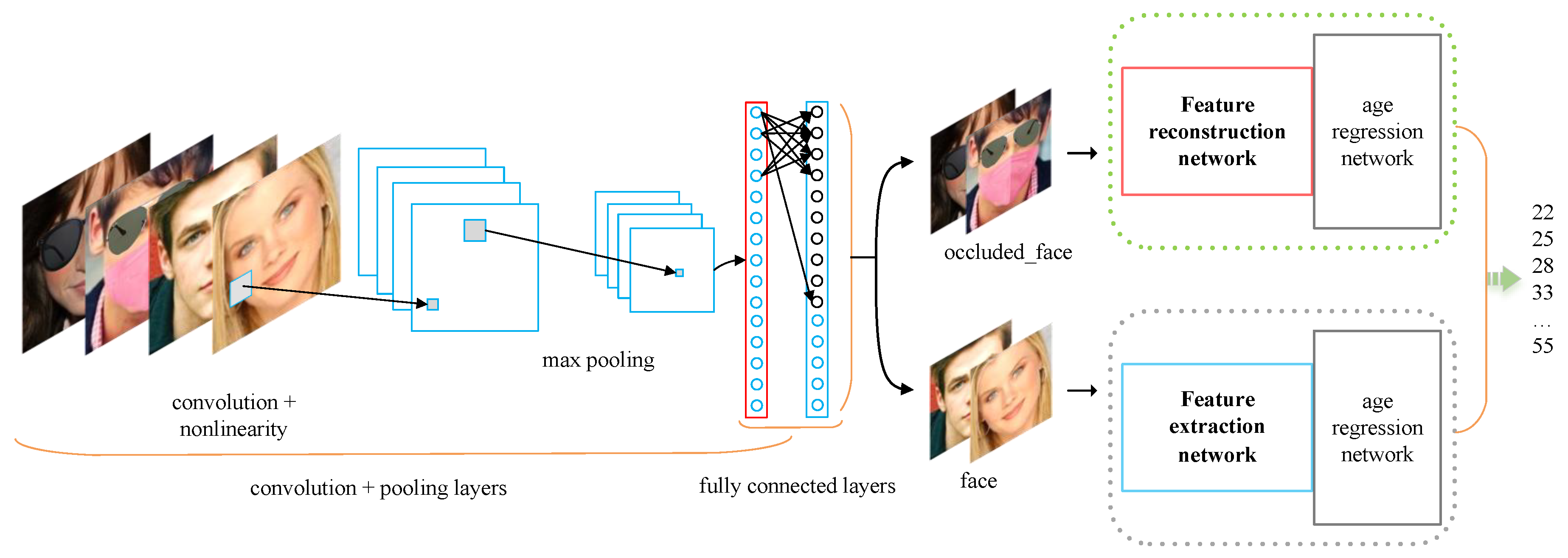
Figure 5.
The performance of the three baseline models on the original dataset and the occluded dataset.
Figure 5.
The performance of the three baseline models on the original dataset and the occluded dataset.
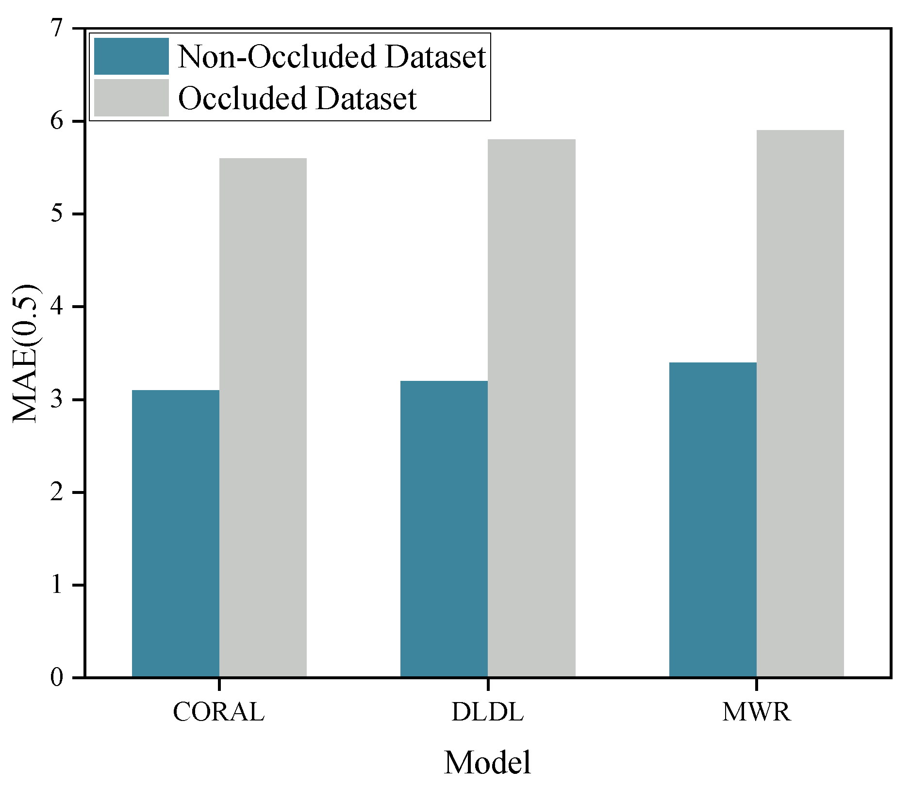
Figure 6.
We tested the impact of various occlusion types, including masks, sunglasses, and masks + glasses, on the age estimation model. The figure shows the MAE performance of the CORAL, DLDL, and MWR models under different occlusion conditions.
Figure 6.
We tested the impact of various occlusion types, including masks, sunglasses, and masks + glasses, on the age estimation model. The figure shows the MAE performance of the CORAL, DLDL, and MWR models under different occlusion conditions.
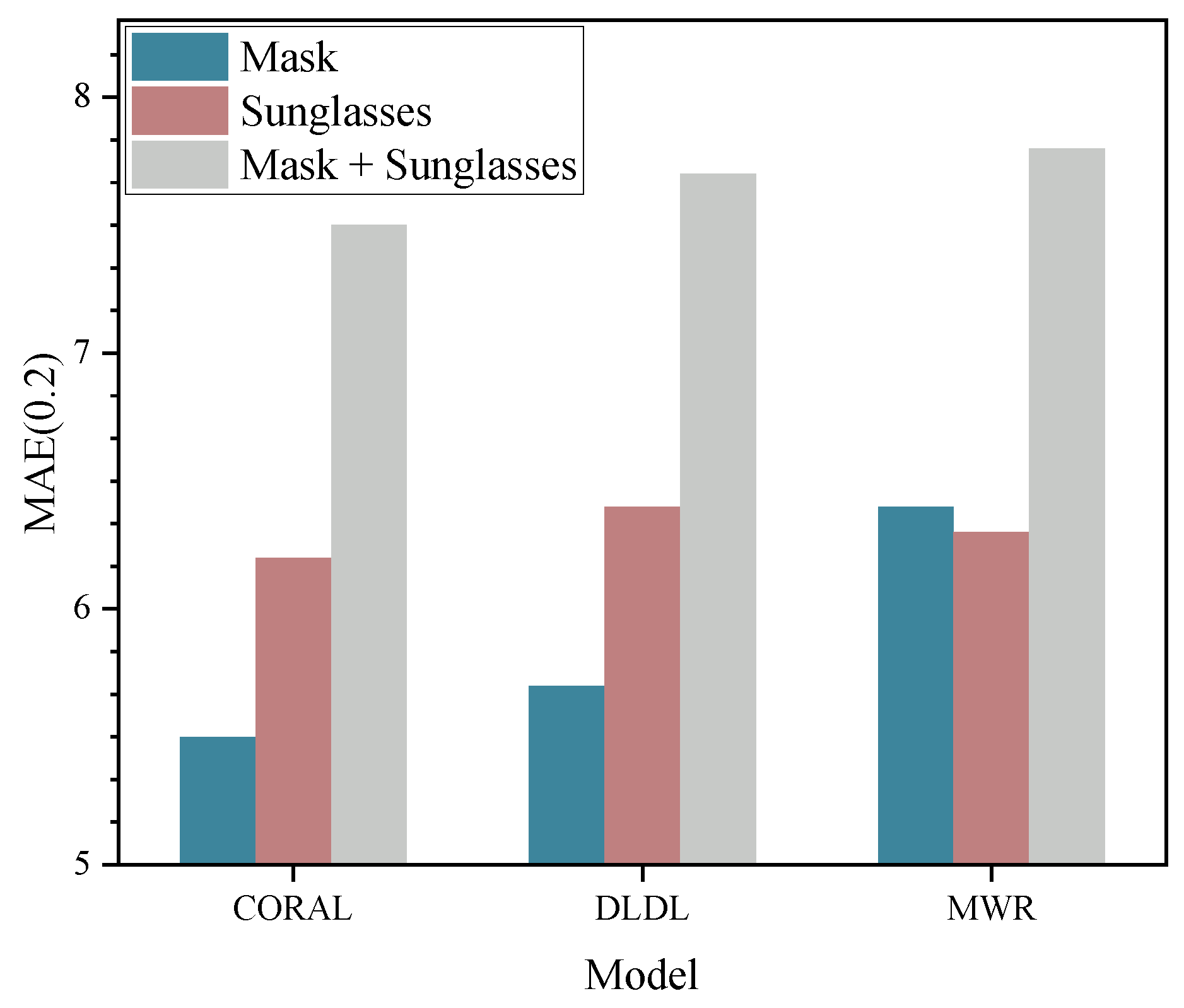
Table 2.
In the MORPH-2 dataset used for training, 77% are African, 19% are European, and the remaining 4% include Hispanic, Asian, Indian, and other ethnicities. The dataset includes 44,692 male images and 10,916 female images. The dataset is divided into 80% for the training set and 20% for the validation set.
| Age Group | 16-20 | 21-25 | 26-30 | 31-35 | 36-40 | 41-45 | 46-50 | 51-55 | 56-60 | 61-65 | 66-70 |
|---|---|---|---|---|---|---|---|---|---|---|---|
| Training Set | 7376 | 7189 | 5748 | 6477 | 6965 | 6914 | 4147 | 2903 | 2000 | 890 | 288 |
| Testing Set | 820 | 800 | 650 | 780 | 750 | 790 | 380 | 180 | 70 | 30 | 20 |
| Total | 8196 | 7989 | 6398 | 7257 | 7715 | 7704 | 4527 | 3083 | 2070 | 920 | 308 |
Note: The table shows the distribution of age groups across the training and testing sets.
Table 3.
Comparison of MAE under different occlusion types.
| Occlusion Type | MAE | ||
|---|---|---|---|
| CORAL | DLDL | MWR | |
| Mask | 5.51 | 5.72 | 6.44 |
| Sunglasses | 6.21 | 6.44 | 6.32 |
| Mask + Sunglasses | 7.52 | 7.71 | 7.82 |
| Mouth Color Block | 4.96 | 4.85 | 5.57 |
| Eyes Color Block | 5.09 | 5.22 | 5.98 |
| Mouth + Eyes Color Block | 6.62 | 6.31 | 7.02 |
Table 8.
MAE of the models before and after global fine-tuning with original age labels.
| Model | MAE | |
|---|---|---|
| Occlusion Dataset Direct Training | Layer-wise Feature Reconstruction + Age Label Fine-tuning | |
| CORAL | 5.61 | 4.27 |
| DLDL | 5.91 | 4.43 |
| MWR | 5.98 | 4.87 |
Table 9.
Cross-dataset evaluation method to verify the generalization performance of the model (Training data: MORPH-2). We count cumulative scores for age errors within a 5-year range.
Table 9.
Cross-dataset evaluation method to verify the generalization performance of the model (Training data: MORPH-2). We count cumulative scores for age errors within a 5-year range.
| Method | AFAD | CACD | IMDB-WIKI | Average | ||||
|---|---|---|---|---|---|---|---|---|
| MAE | CS(%) | MAE | CS(%) | MAE | CS(%) | MAE | CS(%) | |
| Human workers | 8.53 | 48.26 | 8.95 | 46.18 | 9.58 | 44.37 | 9.02 | 46.27 |
| DLP-CNN [48] | 7.86 | 56.58 | 7.98 | 52.33 | 8.92 | 49.37 | 8.25 | 52.76 |
| Pix2Pix [49] | 6.18 | 65.22 | 6.33 | 63.36 | 6.81 | 61.62 | 6.44 | 63.40 |
| DeepFill v2 [50] | 5.92 | 69.39 | 6.06 | 67.86 | 6.61 | 63.83 | 6.20 | 67.03 |
| LCA-GAN [1] | 4.72 | 79.69 | 5.21 | 75.25 | 5.98 | 70.83 | 5.30 | 75.26 |
| MCGRL[6] | 5.11 | 78.86 | 5.48 | 74.22 | 5.81 | 71.09 | 5.47 | 74.72 |
| KD-CORAL (ours) | 4.83 | 77.11 | 5.15 | 74.29 | 5.71 | 72.16 | 5.23 | 74.52 |
| KD-DLDL (ours) | 5.04 | 75.59 | 5.59 | 73.33 | 6.04 | 70.97 | 5.56 | 73.30 |
| KD-MWR (ours) | 5.28 | 74.68 | 5.66 | 72.85 | 6.37 | 70.03 | 5.77 | 72.52 |
Note: The best performance is highlighted in bold.
Disclaimer/Publisher’s Note: The statements, opinions and data contained in all publications are solely those of the individual author(s) and contributor(s) and not of MDPI and/or the editor(s). MDPI and/or the editor(s) disclaim responsibility for any injury to people or property resulting from any ideas, methods, instructions or products referred to in the content. |
© 2025 by the authors. Licensee MDPI, Basel, Switzerland. This article is an open access article distributed under the terms and conditions of the Creative Commons Attribution (CC BY) license (http://creativecommons.org/licenses/by/4.0/).
Copyright: This open access article is published under a Creative Commons CC BY 4.0 license, which permit the free download, distribution, and reuse, provided that the author and preprint are cited in any reuse.


