New Three Different Generators for Constructing New Three Different Bivariate Copulas

Iman Attia

doi:10.20944/preprints202504.1456.v1

Submitted:

16 April 2025

Posted:

17 April 2025

Read the latest preprint version here

Abstract

In this paper, the author introduces new methods to construct Archimedean copulas. The generator of each copula fulfills the sufficient conditions as regards the boundary and being continuous, decreasing, and convex. Each inverse generator also fulfills the necessary conditions as regards the boundary conditions, marginal uniformity, and 2-increasing properties. Although these copulas satisfy these conditions, they have some limitations. They do not cover the entire dependency spectrum, ranging from perfect negative dependency to perfect positive dependency, passing through the independence state. Even the third copula has a fixed constant Kendall tau measure and fixed values for both the joint CDF and PDF copula, but the generator output changes with the changing value of the dependency parameter. For each copula, the author discusses the derivation, the properties, whether it has a singular part or not, and the Kendall tau measure for dependency. The article shows figures for depicting the generator function, joint CDF, and joint PDF for each copula.

Keywords:

Archimedean copula

;

generator

;

inverse generator

;

MBUR

;

Kendall tau

Subject:

Computer Science and Mathematics - Applied Mathematics

Introduction

Copula can express the nonlinear dependency between two or more variables, in comparison with correlation that can capture linear dependency between variables. It is a technique used to implement the joint distribution of the many variables (two or more). This has many wide applications in modern era of science like hydrology and geophysics (Valle & Kaplan, 2019) (Liu et al., 2018) (Salvadori et al., 2007), transportation research(Ma et al., 2017) (Bhat & Eluru, 2009) , medicine (Kuss et al., 2014) (Lapuyade-Lahorgue et al., 2017) (Gomes et al., 2019) , engineering (Kilgore & Thompson, 2011), biology (Konigorski et al., 2014) (Dokuzoğlu & Purutçuoğlu, 2017), climate research (Schölzel & Friederichs, 2008) (Oppenheimer et al., 2016), economics (Oh & Patton, 2018) (Kole et al., 2007) (De Lira Salvatierra & Patton, 2015). Sklar (Abe Sklar, 1973) showed that a copula exists for any multivariate distribution, such that the joibt distribution equals the copula applied to the marginal.

Definition 1

(Sklar’s theorem 1): For any bivariate distribution function F with marginal

F_{1}

and

F_{2}

, there exists a copula such that

F (x, y) = C (F_{1} (x), F_{2} (y)), x, y \in \bar{R} = R \cup \{- \infty, \infty\}

If F is continuous, then the copula C is unique. Otherwise, it is uniquely determined on the

F_{1} (\bar{R}) \times F_{2} (\bar{R})

. The converse is also true, for any copula and univariate distribution functions

F_{1}

and

F_{2}

, the function

C (F_{1} (x), F_{2} (y))

is a bivariate distribution function with margins

F_{1}

and

F_{2}

.

A bivariate distribution function

C (u, v)

with marginal

u = F_{X} (x)

and

v = F_{Y} (y)

is said to be generated by an Archimedean copula, if it can be written in the form of equation (1)

C (u, v) = φ^{- 1} (φ (u) + φ (v))

(1)

The generator

φ (u)

should satisfy the following conditions (sufficient conditions):

(1): $φ (u)$ is continuous, strictly decreasing and convex function mapping $[0,1]$ onto $[0, \infty)$ , in other words , $φ^{'} (u) < 0$ ( decreasing) and $φ^{''} (u) > 0$ ( convex)
(2): $φ (0) = \infty$
(3): $φ (1) = 0$

Definition 2

: a bivariate copula is a non-decreasing and a right-continuous bivariate function mapping

C : [0,1] \times [0,1] \to [0,1]

which satisfies the following conditions

(1): $C (0, v) = C (u, 0) = 0, \forall (u, v) \in {[0,1]}^{2}$ ( Grounded)
(2): $C (1, v) = v$ and $C (u, 1) = u$ $\forall (u, v) \in {[0,1]}^{2}$ ( uniform marginal)
(3): $C (u_{1}, v_{1}) - C (u_{1}, v_{2}) - C (u_{2}, v_{1}) + C (u_{2}, v_{2}) \geq 0, f o r u_{1} > u_{2} a n d v_{1} > v_{2}$ $\forall (u_{1}, u_{2}, v_{1}, v_{2}) \in {[0,1]}^{4}$ (2- increasing) . This last property is equal to $\frac{\partial C (u, v)}{\partial u \partial v} \geq 0$ $\frac{\partial C (u, v)}{\partial u \partial v} = c (u, v)$ the joint PDF of the copula.

So the copula links the marginal distributions through the dependency parameter.

The singular part of the copula is defined by (Genest & Mackay, 1986) in the following Theorem 2: the ratio between the generator and the first derivative of the generator evaluated at zero does not equal zero.

Theorem: the distribution

C (u, v)

generated by

φ

has a singular component iff

\frac{φ (0)}{φ^{'} (0)} \neq 0

in that case,

φ (u) + φ (v) = φ (0)

with probability =

- \frac{φ (0)}{φ^{'} (0)}

This paper is structured in 4 sections. Section 1 discusses the first copula, its derivation, properties and figures for its PDF and CDF. Section 2 explains the second copula with the same items. Section 3 explore the third copula in the same manner. Section 4 illustrate the discussion and conclusion with future work

Section 1: (First Copula)

Let’s say the inverse generator is

{C (φ (u) + φ (v)) = Φ}^{- 1} (t) = z = e x p (\frac{{- t}^{α}}{α})

The generator is the:

\ln Φ^{- 1} (t) = \ln \{e x p (\frac{{- t}^{α}}{α})\} = \frac{{- t}^{α}}{α} - α l n Φ^{- 1} (t) = t^{α} {φ (z) = (- α l n Φ^{- 1} (t))}^{\frac{1}{α}} = {(- α l n (z))}^{\frac{1}{α}} = t, z \in (0,1)

The generator should fulfill the sufficient conditions:

(1): $φ (0) = {(- α ln 0)}^{\frac{1}{α}} = \infty$
(2): $φ (1) = {(- α ln 1)}^{\frac{1}{α}} = 0$
(3): $φ^{'} (z) = \frac{1}{α} {(- α \ln z)}^{\frac{1}{α} - 1} (\frac{- α}{z}) = {(- α \ln z)}^{\frac{1}{α} - 1} (\frac{- 1}{z}) < 0$

This ensures that the generator is a decreasing function.
(4): $φ^{''} (z) = (\frac{1}{α} - 1) {(- α \ln z)}^{\frac{1}{α} - 2} (\frac{- α}{z}) (\frac{- 1}{z}) + {(- α \ln z)}^{\frac{1}{α} - 1} (\frac{1}{z^{2}}) > 0$

This ensures that the generator is convex for

0 < α \leq 1

.

for bivariate distribution:

{φ (u) = (- α ln u)}^{\frac{1}{α}} {φ (v) = (- α ln v)}^{\frac{1}{α}} φ (w) = φ (u) + φ (v) = {(- α ln u)}^{\frac{1}{α}} + {(- α ln v)}^{\frac{1}{α}} C (φ (u) + φ (v)) = e x p ({- \frac{1}{α} [{(- α ln u)}^{\frac{1}{α}} + {(- α ln v)}^{\frac{1}{α}}]}^{α}) C (u, v) = C (F_{X} (x), F_{Y} (y))

For a copula to be valid copula it should fulfill the boundary condition, the marginal uniformity and 2- increasing condition. And this is equivalent for the inverse generator the necessary conditions to be fulfilled are the following:

Proposition 1

: The boundary conditions and marginal uniformity:

C (0, v) = C (u, 0) = 0

, boundary condition.

C (1, v) = v a n d C (u, 1) = u

, the marginal uniformity.

Proof :

C (1, v) = e x p ({- \frac{1}{α} [{(- α ln (1))}^{\frac{1}{α}} + {(- α ln v)}^{\frac{1}{α}}]}^{α}) C (1, v) = e x p ({- \frac{1}{α} [0 + {(- α ln v)}^{\frac{1}{α}}]}^{α}) C (1, v) = e x p ({- \frac{1}{α} [{(- α ln v)}^{\frac{1}{α}}]}^{α}) = e x p (\frac{- α ln v}{- α}) = v C (u, 1) = e x p ({- \frac{1}{α} [{(- α ln u)}^{\frac{1}{α}}]}^{α}) = e x p (\frac{- α ln u}{- α}) = u

Proposition 2

: for copula to be valid it should be 2-increasing, in other words,

\frac{\partial^{2} C (u, v)}{\partial u \partial v} \geq 0

Proof:

\frac{\partial C (u, v)}{\partial u} = e x p ({- \frac{1}{α} [{(- α ln (u))}^{\frac{1}{α}} + {(- α ln v)}^{\frac{1}{α}}]}^{α}) \times (\frac{- 1}{α}) (α) {[{(- α ln (u))}^{\frac{1}{α}} + {(- α ln v)}^{\frac{1}{α}}]}^{α - 1} (\frac{1}{α} {(- α ln (u))}^{\frac{1}{α} - 1} (\frac{- α}{u})) \frac{\partial C (u, v)}{\partial u} = e x p ({- \frac{1}{α} [{(- α ln (u))}^{\frac{1}{α}} + {(- α ln v)}^{\frac{1}{α}}]}^{α}) \times {[{(- α ln (u))}^{\frac{1}{α}} + {(- α ln v)}^{\frac{1}{α}}]}^{α - 1} ({(- α ln (u))}^{\frac{1}{α} - 1} (\frac{1}{u})) \frac{\partial}{\partial v} (\frac{\partial C (u, v)}{\partial u}) = e x p ({- \frac{1}{α} [{(- α ln (u))}^{\frac{1}{α}} + {(- α ln v)}^{\frac{1}{α}}]}^{α}) \times (\frac{- 1}{α}) (α) {[{(- α \ln (u))}^{\frac{1}{α}} + {(- α ln v)}^{\frac{1}{α}}]}^{α - 1} (\frac{1}{α} {(- α \ln (v))}^{\frac{1}{α} - 1} (\frac{- α}{v})) \times {[{(- α \ln (u))}^{\frac{1}{α}} + {(- α ln v)}^{\frac{1}{α}}]}^{α - 1} ({(- α ln (u))}^{\frac{1}{α} - 1} (\frac{1}{u})) + e x p ({- \frac{1}{α} [{(- α ln (u))}^{\frac{1}{α}} + {(- α ln v)}^{\frac{1}{α}}]}^{α}) ({(- α ln (u))}^{\frac{1}{α} - 1} (\frac{1}{u})) \times {(α - 1) [{(- α ln (u))}^{\frac{1}{α}} + {(- α ln v)}^{\frac{1}{α}}]}^{α - 2} (\frac{1}{α} {(- α ln (v))}^{\frac{1}{α} - 1} (\frac{- α}{v})) = e x p ({- \frac{1}{α} [{(- α ln (u))}^{\frac{1}{α}} + {(- α ln v)}^{\frac{1}{α}}]}^{α}) {[{(- α ln (u))}^{\frac{1}{α}} + {(- α ln v)}^{\frac{1}{α}}]}^{2 α - 2} ({(- α ln (v))}^{\frac{1}{α} - 1} (\frac{1}{v})) \times ({(- α ln (u))}^{\frac{1}{α} - 1} (\frac{1}{u})) + e x p ({- \frac{1}{α} [{(- α ln (u))}^{\frac{1}{α}} + {(- α ln v)}^{\frac{1}{α}}]}^{α}) ({(- α ln (u))}^{\frac{1}{α} - 1} (\frac{1}{u})) \times {(α - 1) [{(- α ln (u))}^{\frac{1}{α}} + {(- α ln v)}^{\frac{1}{α}}]}^{α - 2} ({(- α ln (v))}^{\frac{1}{α} - 1} (\frac{- 1}{v})) = e x p ({- \frac{1}{α} [{(- α ln (u))}^{\frac{1}{α}} + {(- α ln v)}^{\frac{1}{α}}]}^{α}) {[{(- α ln (u))}^{\frac{1}{α}} + {(- α ln v)}^{\frac{1}{α}}]}^{α - 2} [\frac{{(α^{2} \ln v \ln u)}^{\frac{1}{α} - 1}}{v u}] \times \{{[{(- α ln (u))}^{\frac{1}{α}} + {(- α ln v)}^{\frac{1}{α}}]}^{α} - (α - 1)\} = e x p ({- \frac{1}{α} [{(- α ln (u))}^{\frac{1}{α}} + {(- α ln v)}^{\frac{1}{α}}]}^{α}) {[{(- α ln (u))}^{\frac{1}{α}} + {(- α ln v)}^{\frac{1}{α}}]}^{α - 2} [\frac{{(α^{2} \ln v \ln u)}^{\frac{1}{α} - 1}}{v u}] \times \{{[{(- α ln (u))}^{\frac{1}{α}} + {(- α ln v)}^{\frac{1}{α}}]}^{α} + 1 - α\}

Although the second derivative is positive at the following intervals:

(0,1]

so alpha can be defined on the interval

0 < α \leq 1

.

Proposition 3

: this copula is absolutely continuous copula and it has no singular part.

Proof:

to test for singularity:

\frac{φ (0)}{φ^{'} (0)} = 0

\frac{φ (u)}{φ^{'} (u)} = \frac{{(- α ln u)}^{\frac{1}{α}}}{{\frac{1}{α} (- α ln u)}^{\frac{1}{α} - 1} (\frac{- α}{u})} = \frac{- α ln u}{\frac{- 1}{u}} \lim_{u \to 0} \frac{φ (u)}{φ^{'} (u)} = \frac{{(- α ln u)}^{\frac{1}{α}}}{{\frac{1}{α} (- α ln u)}^{\frac{1}{α} - 1} (\frac{- α}{u})} = \frac{- α ln u}{\frac{- 1}{u}}

Using L’Hopital

\lim_{u \to 0} \frac{φ (u)}{φ^{'} (u)} = \underset{u \to 0}{l i m} \frac{{(- α ln u)}^{\frac{1}{α}}}{{\frac{1}{α} (- α ln u)}^{\frac{1}{α} - 1} (\frac{- α}{u})} = \underset{u \to 0}{l i m} \frac{\frac{α}{u}}{\frac{- 1}{u^{2}}} = \underset{u \to 0}{l i m} (- α u) = - α (0) = 0

As long as this limit is zero at u=0 so it has no singular part and it is absolutely continuous copula.

Proposition 4

: Kendall tau for this copula is τ = 1 − α

Proof:

τ = 4 \int_{0}^{1} \frac{φ (u)}{φ^{'} (u)} d u + 1 \int_{0}^{1} \frac{φ (u)}{φ^{'} (u)} d u = \int_{0}^{1} α u \ln (u) d u = \frac{- α}{4}, i n t e g r a t i o n b y p a r t s τ = 4 \int_{0}^{1} \frac{φ (u)}{φ^{'} (u)} d u + 1 = 4 (\frac{- α}{4}) + 1 = 1 - α

If

α = 1 τ = 0

indicating independence.

Although the second derivative is positive at the following intervals:

(0,1]

considering that tau is defined within the interval

[- 1,1]

so alpha can be defined on the interval

0 < α \leq 1

. In this interval the Kendall tau can show positive dependency and independency.

Preposition 5

: This copula is product copula at alpha =1, in other word, if alpha=1,

C (u, v) = u v

, this is the product copula indicating independency.

Proof:

C (u, v) = e x p ({- \frac{1}{α} [{(- α ln u)}^{\frac{1}{α}} + {(- α ln v)}^{\frac{1}{α}}]}^{α}) = e x p (- [- \ln u - \ln v]) e x p ([\ln u + \ln v]) = e x p ([\ln u v]) = u v C (u, v) = u v

The following figures illustrates the Copula surface with different alpha values

Figure 1. shows the generator function (decreasing and convex) at alpha = 0.6.

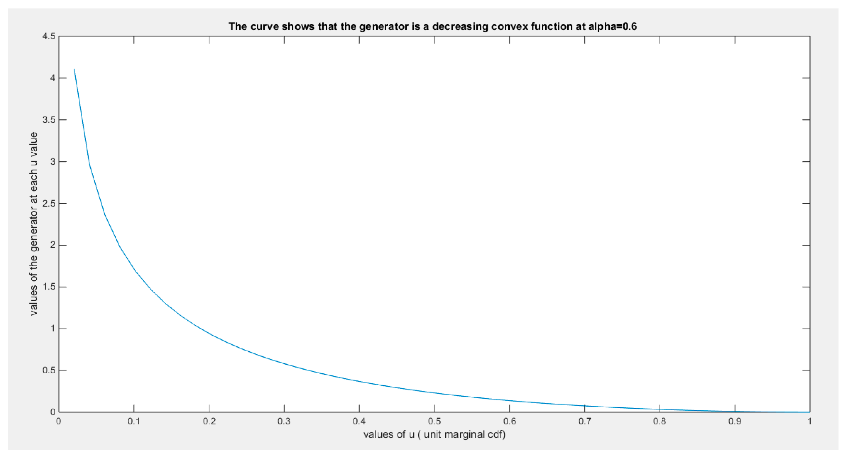
Figure 2. shows the joint PDF copula (copula density) at alpha=0.1.

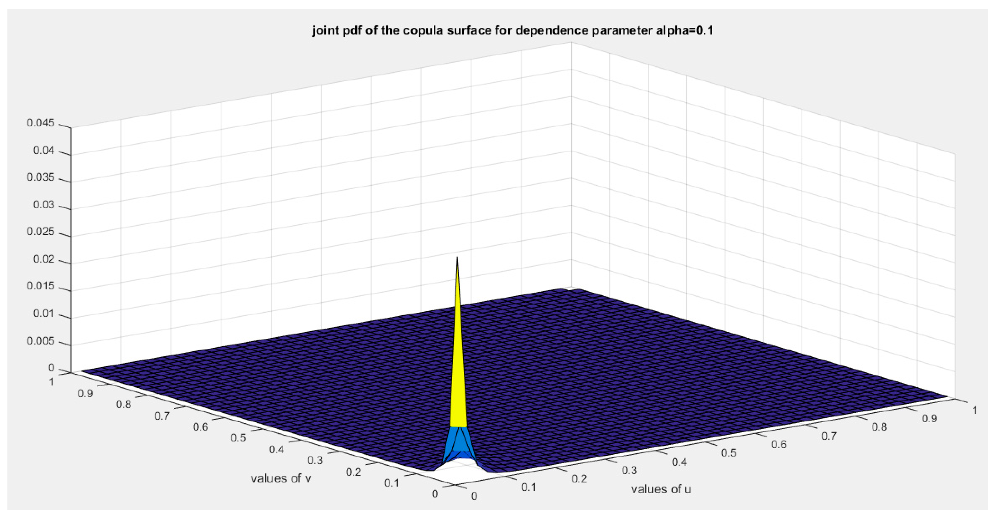
Figure 3. shows the joint CDF copula (Copula) at alpha =0.1.

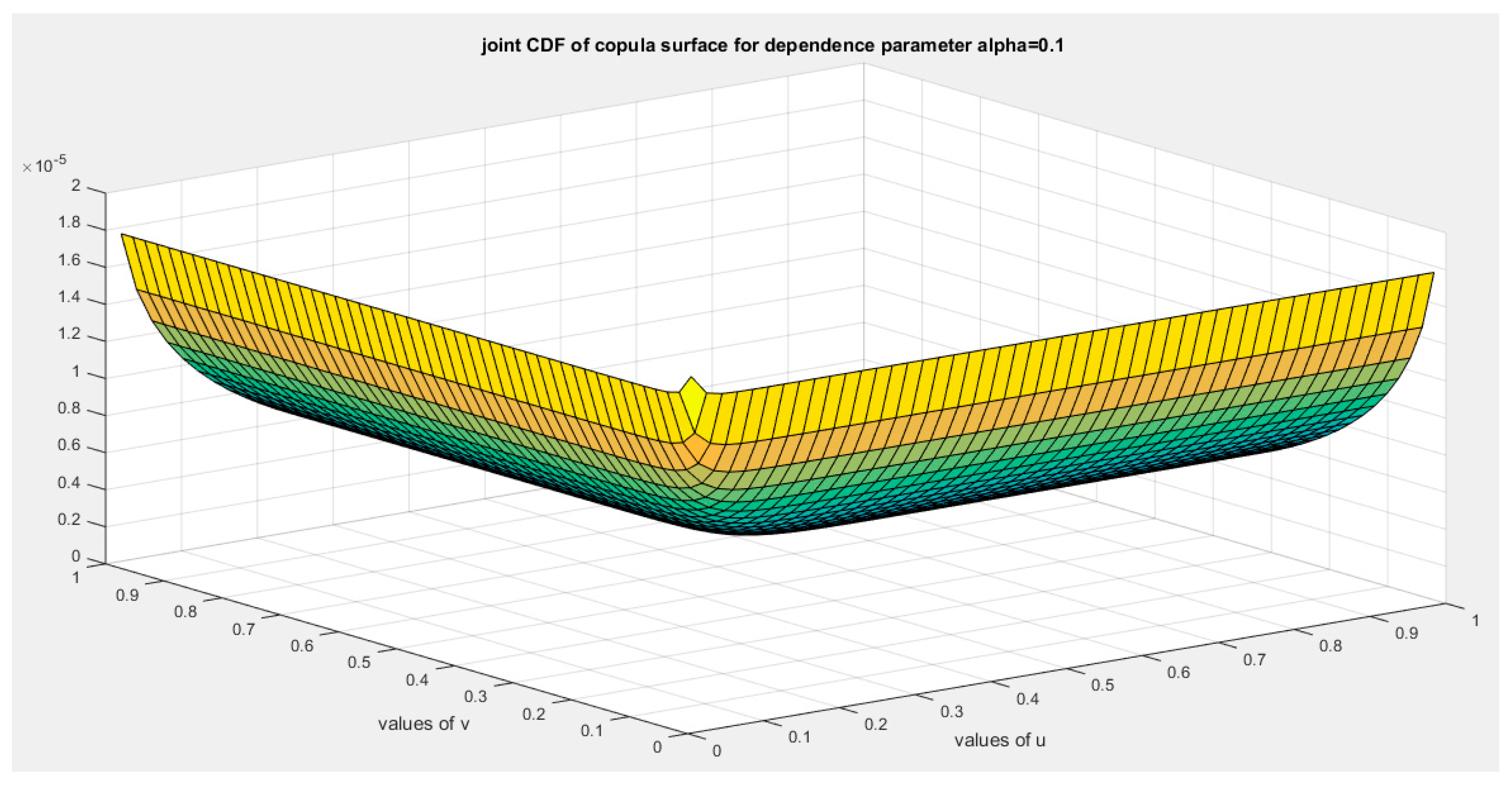
Figure 4. shows the joint pdf copula ( copula density) at alpha=0.6.

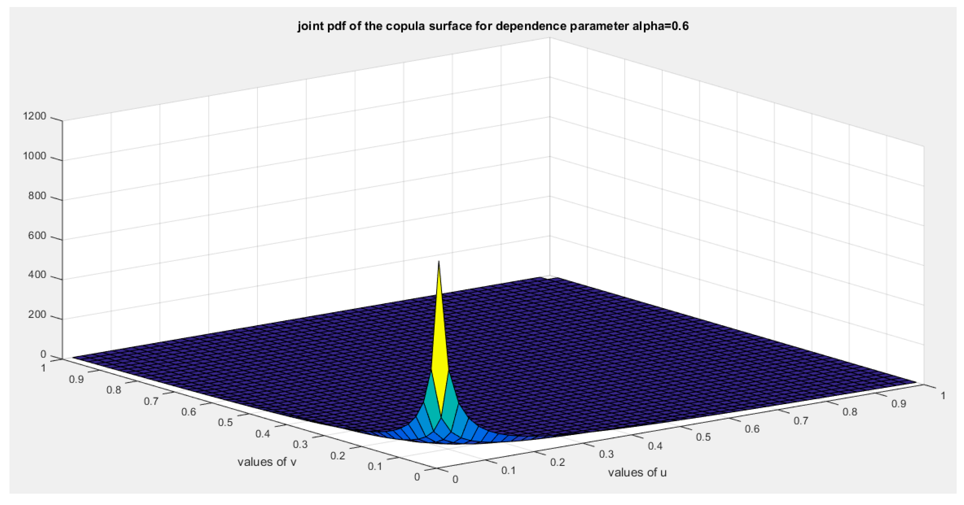
Figure 5. shows the joint cdf copula ( Copula) at alpha=0.6.

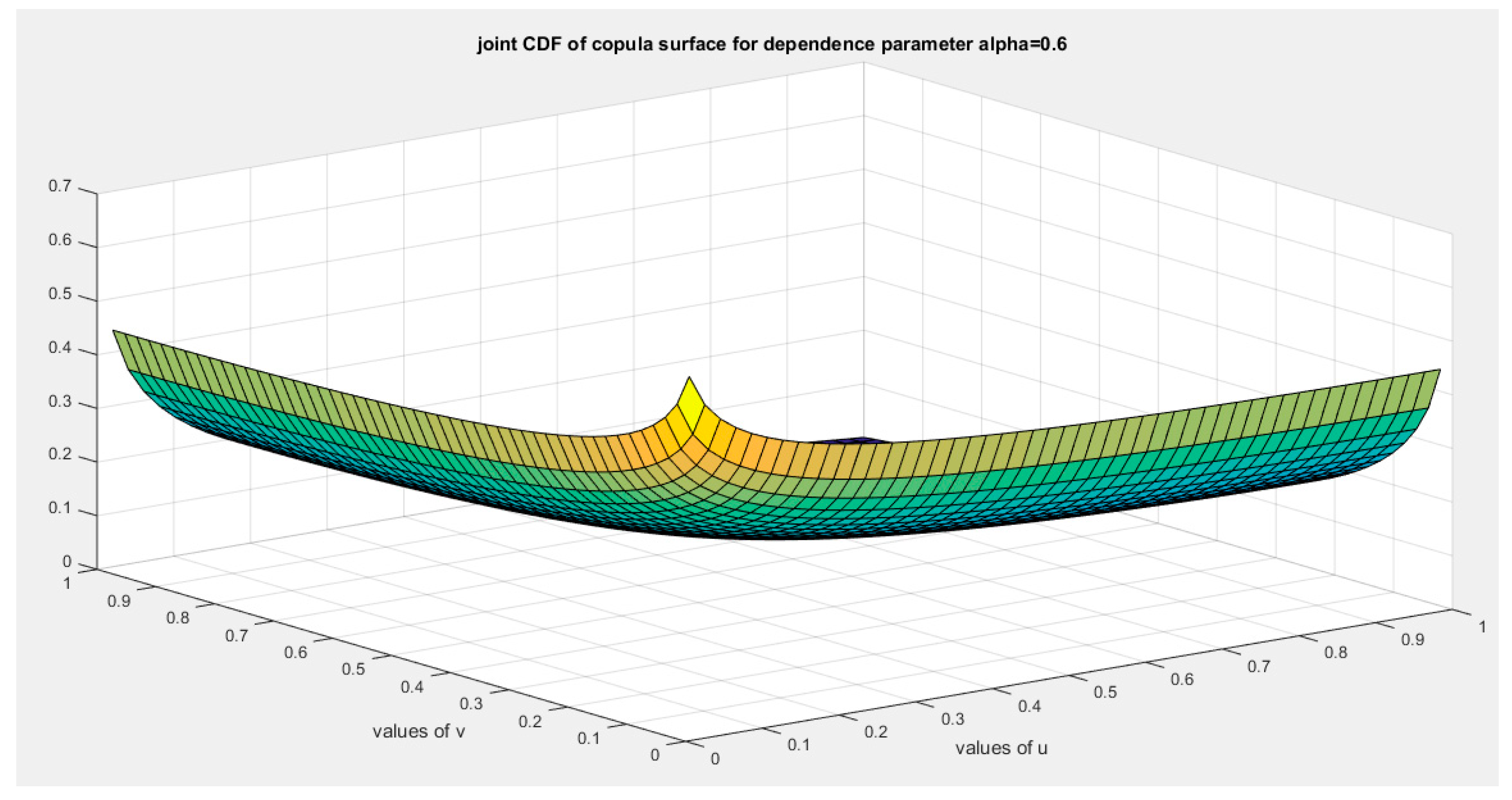
Figure 6. shows the joint pdf copula ( copula density) at alpha =1.

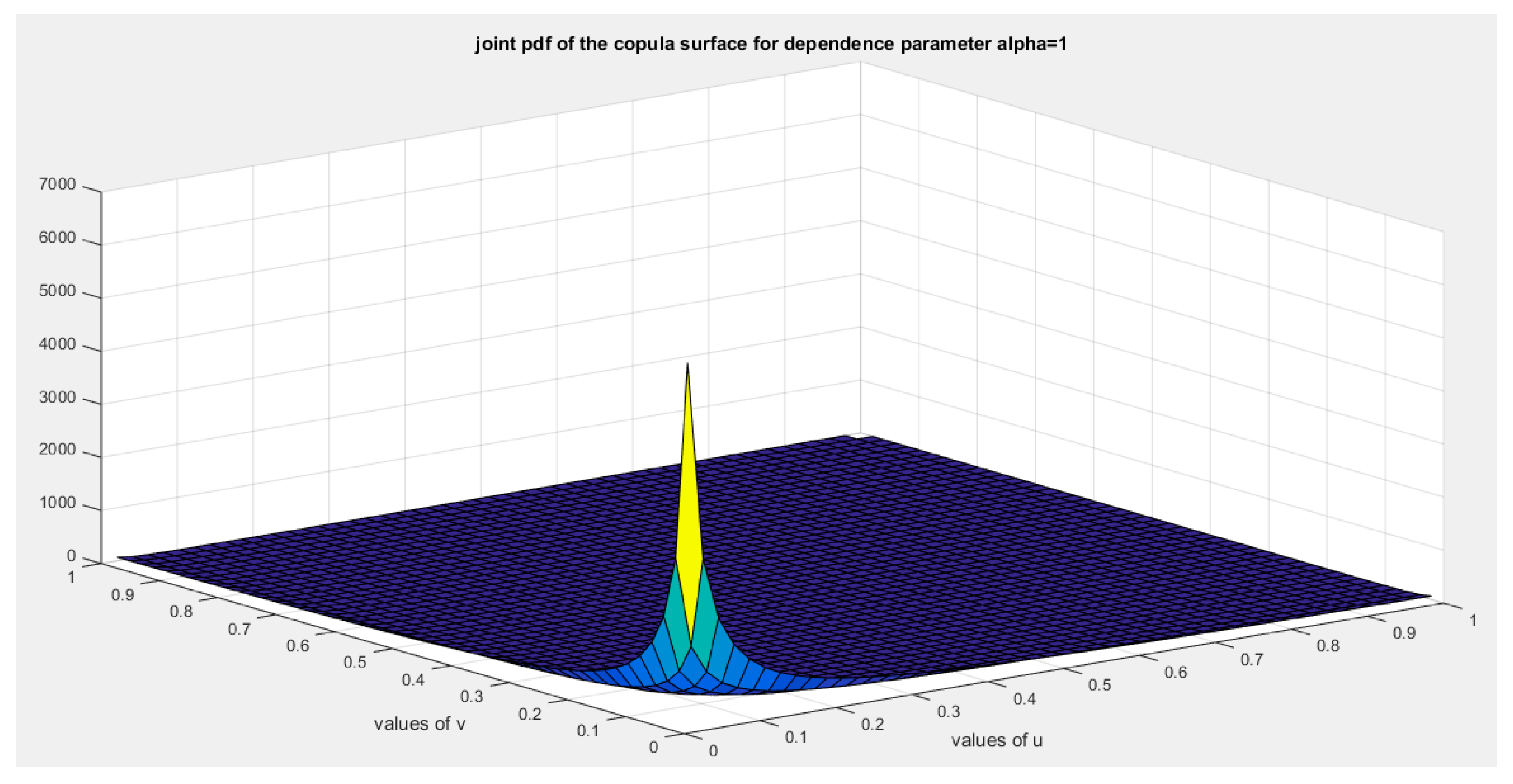
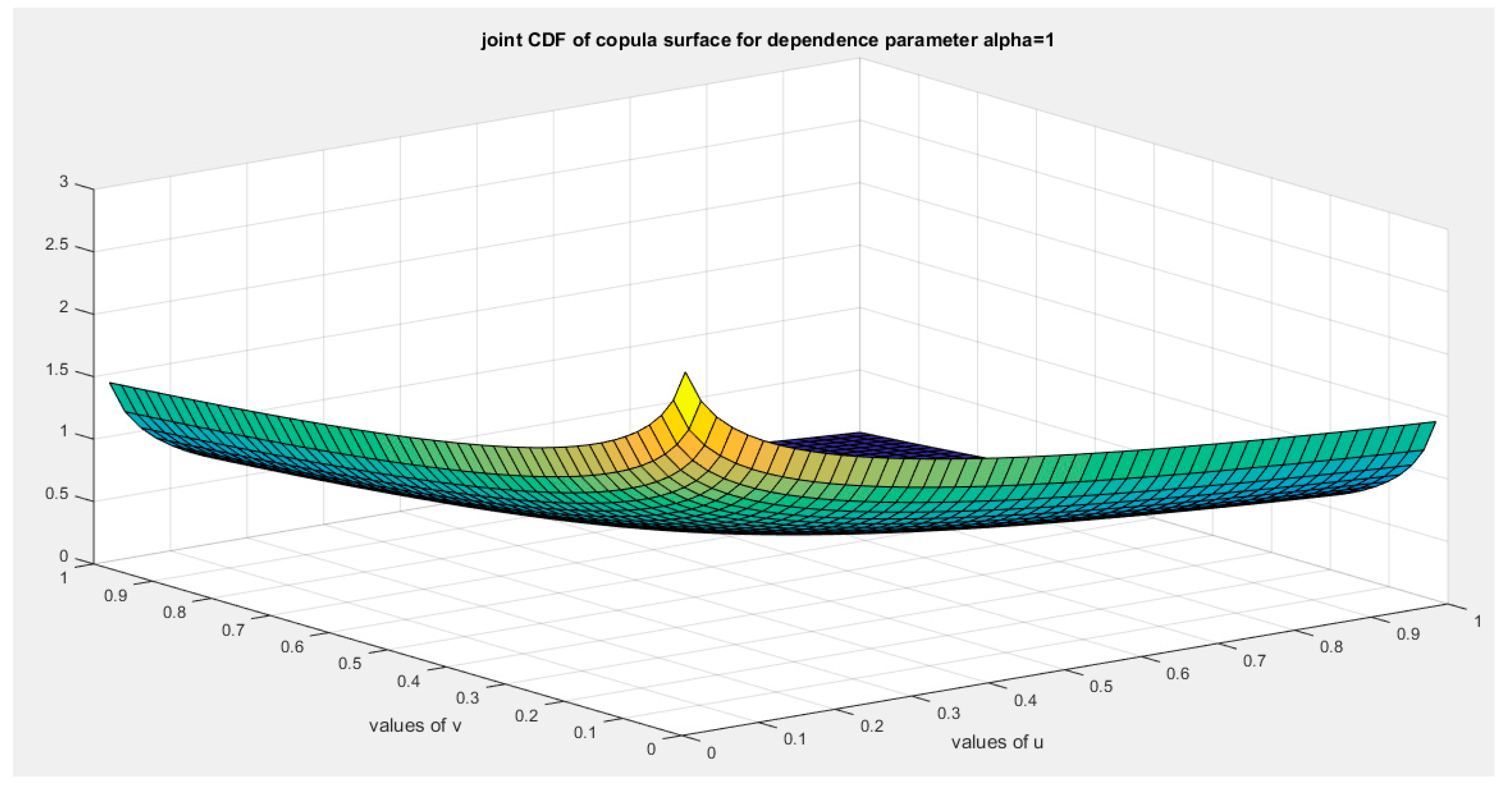
Figure 7. shows joint cdf Copula ( Copula) at alpha=1.

The limitation for this copula is that it does not cover the negative dependency between variables.

Section 2: (Second Copula)

Let’s say the inverse generator is

{C (φ (u) + φ (v)) = Φ}^{- 1} (t) = z = e x p ({- t}^{α^{2}})

The generator is:

\ln z = \ln \{e x p ({- t}^{α^{2}})\} = {- t}^{α^{2}} - \ln z = t^{α^{2}} {φ (z) = (- \ln z)}^{α^{- 2}} = t, z \in (0,1)

The generator should fulfill the sufficient conditions:

(1): $φ (0) = {(- \ln 0)}^{α^{- 2}} = \infty$
(2): $φ (1) = {(- \ln 1)}^{α^{- 2}} = 0$
(3): $φ^{'} (z) = α^{- 2} {(- \ln z)}^{α^{- 2} - 1} (\frac{- 1}{z}) < 0$

This ensures that the generator is a decreasing function.
(4): $φ^{''} (z) = \frac{1}{α^{2}} (\frac{1}{α^{2}} - 1) {(- \ln z)}^{α^{- 2} - 2} (\frac{- 1}{z}) (\frac{- 1}{z}) + α^{- 2} {(- \ln z)}^{α^{- 2} - 1} (\frac{1}{z^{2}}) > 0$

This ensures that the generator is convex at

0 < α \leq 1

for bivariate distribution:

{φ (u) = (- \ln u)}^{\frac{1}{α^{2}}} {φ (v) = (- \ln v)}^{\frac{1}{α^{2}}} φ (w) = φ (u) + φ (v) = {(- \ln u)}^{\frac{1}{α^{2}}} + {(- \ln v)}^{\frac{1}{α^{2}}} C (φ (u) + φ (v)) = e x p ({- [{(- \ln u)}^{\frac{1}{α^{2}}} + {(- \ln v)}^{\frac{1}{α^{2}}}]}^{α^{2}}) C (u, v) = C (F_{X} (x), F_{Y} (y))

For a copula to be a valid copula it should fulfill the boundary condition, the marginal uniformity and 2- increasing condition. And this is equivalent for necessary conditions of the inverse generator to be fulfilled which are the following:

Proposition 6

: The boundary conditions and marginal uniformity:

C (0, v) = C (u, 0) = 0

, boundary condition.

C (1, v) = v a n d C (u, 1) = u

, the marginal uniformity.

Proof:

C (1, v) = e x p ({- [{(- \ln 1)}^{\frac{1}{α^{2}}} + {(- \ln v)}^{\frac{1}{α^{2}}}]}^{α^{2}}) C (1, v) = e x p ({- [0 + {(- \ln v)}^{\frac{1}{α^{2}}}]}^{α^{2}}) C (1, v) = e x p ({- [{(- \ln v)}^{\frac{1}{α^{2}}}]}^{α^{2}}) = e x p (- [- \ln v]) = v C (u, 1) = e x p ({- [{(- \ln u)}^{\frac{1}{α^{2}}}]}^{α^{2}}) = e x p (- [- \ln u]) = u

Proposition 7

: for copula to be valid it should be 2-increasing, in other words

\frac{\partial^{2} C (u, v)}{\partial u \partial v} \geq 0

Proof:

\frac{\partial C (u, v)}{\partial u} = e x p ({- [{(- \ln u)}^{\frac{1}{α^{2}}} + {(- \ln v)}^{\frac{1}{α^{2}}}]}^{α^{2}}) \times (- α^{2}) {[{(- \ln u)}^{\frac{1}{α^{2}}} + {(- \ln v)}^{\frac{1}{α^{2}}}]}^{α^{2} - 1} (\frac{1}{α^{2}} {(- \ln (u))}^{\frac{1}{α^{2}} - 1} (\frac{- 1}{u})) \frac{\partial C (u, v)}{\partial u} = {e x p ({- [{(- \ln u)}^{\frac{1}{α^{2}}} + {(- \ln v)}^{\frac{1}{α^{2}}}]}^{α^{2}}) [{(- \ln u)}^{\frac{1}{α^{2}}} + {(- \ln v)}^{\frac{1}{α^{2}}}]}^{α^{2} - 1} ({(- \ln (u))}^{\frac{1}{α^{2}} - 1} (\frac{1}{u})) \frac{\partial}{\partial v} (\frac{\partial C (u, v)}{\partial u}) = e x p ({- [{(- \ln u)}^{\frac{1}{α^{2}}} + {(- \ln v)}^{\frac{1}{α^{2}}}]}^{α^{2}}) \times (- α^{2}) {[{(- \ln u)}^{\frac{1}{α^{2}}} + {(- \ln v)}^{\frac{1}{α^{2}}}]}^{α^{2} - 1} (\frac{1}{α^{2}} {(- \ln (v))}^{\frac{1}{α^{2}} - 1} (\frac{- 1}{v})) \times {[{(- \ln u)}^{\frac{1}{α^{2}}} + {(- \ln v)}^{\frac{1}{α^{2}}}]}^{α^{2} - 1} ({(- \ln (u))}^{\frac{1}{α^{2}} - 1} (\frac{1}{u})) + e x p ({- [{(- \ln u)}^{\frac{1}{α^{2}}} + {(- \ln v)}^{\frac{1}{α^{2}}}]}^{α^{2}}) ({(- \ln (u))}^{\frac{1}{α^{2}} - 1} (\frac{1}{u})) \times (α^{2} - 1) {[{(- \ln u)}^{\frac{1}{α^{2}}} + {(- \ln v)}^{\frac{1}{α^{2}}}]}^{α^{2} - 2} (\frac{1}{α^{2}} {(- \ln (v))}^{\frac{1}{α^{2}} - 1} (\frac{- 1}{v})) = e x p ({- [{(- \ln u)}^{\frac{1}{α^{2}}} + {(- \ln v)}^{\frac{1}{α^{2}}}]}^{α^{2}}) \times {[{(- \ln u)}^{\frac{1}{α^{2}}} + {(- \ln v)}^{\frac{1}{α^{2}}}]}^{α^{2} - 1} ({(- \ln (v))}^{\frac{1}{α^{2}} - 1} (\frac{1}{v})) \times {[{(- \ln u)}^{\frac{1}{α^{2}}} + {(- \ln v)}^{\frac{1}{α^{2}}}]}^{α^{2} - 1} ({(- \ln (u))}^{\frac{1}{α^{2}} - 1} (\frac{1}{u})) + e x p ({- [{(- \ln u)}^{\frac{1}{α^{2}}} + {(- \ln v)}^{\frac{1}{α^{2}}}]}^{α^{2}}) ({(- \ln (u))}^{\frac{1}{α^{2}} - 1} (\frac{1}{u})) \times (α^{2} - 1) {[{(- \ln u)}^{\frac{1}{α^{2}}} + {(- \ln v)}^{\frac{1}{α^{2}}}]}^{α^{2} - 2} (\frac{1}{α^{2}} {(- \ln (v))}^{\frac{1}{α^{2}} - 1} (\frac{- 1}{v})) = = e x p ({- [{(- \ln u)}^{\frac{1}{α^{2}}} + {(- \ln v)}^{\frac{1}{α^{2}}}]}^{α^{2}}) {[{(- \ln u)}^{\frac{1}{α^{2}}} + {(- \ln v)}^{\frac{1}{α^{2}}}]}^{2 α^{2} - 2} [\frac{{(\ln (v) \ln (u))}^{\frac{1}{α^{2}} - 1}}{u v}] + (α^{2} - 1) (\frac{- 1}{α^{2}}) [\frac{{(\ln (v) \ln (u))}^{\frac{1}{α^{2}} - 1}}{u v}] e x p ({- [{(- \ln u)}^{\frac{1}{α^{2}}} + {(- \ln v)}^{\frac{1}{α^{2}}}]}^{α^{2}}) \times {[{(- \ln u)}^{\frac{1}{α^{2}}} + {(- \ln v)}^{\frac{1}{α^{2}}}]}^{α^{2} - 2} = e x p ({- [{(- \ln u)}^{\frac{1}{α^{2}}} + {(- \ln v)}^{\frac{1}{α^{2}}}]}^{α^{2}}) {[{(- \ln u)}^{\frac{1}{α^{2}}} + {(- \ln v)}^{\frac{1}{α^{2}}}]}^{α^{2} - 2} [\frac{{(\ln (v) \ln (u))}^{\frac{1}{α^{2}} - 1}}{u v}] \times \{{[{(- \ln u)}^{\frac{1}{α^{2}}} + {(- \ln v)}^{\frac{1}{α^{2}}}]}^{α^{2}} - (\frac{1}{α^{2}}) (α^{2} - 1)\}

The second derivative is positive at

(0,1]

Preposition 8

: this copula is absolutely continuous copula and it has no singular part.

Proof:

to test for singularity:

\frac{φ (0)}{φ^{'} (0)} = 0

\frac{φ (u)}{φ^{'} (u)} = \frac{{(- \ln u)}^{\frac{1}{α^{2}}}}{{\frac{1}{α^{2}} (- \ln u)}^{\frac{1}{α^{2}} - 1} (\frac{- 1}{u})} = \frac{α^{2} (- \ln u)}{\frac{- 1}{u}} \lim_{u \to 0} \frac{φ (u)}{φ^{'} (u)} = \underset{u \to 0}{l i m} \frac{{(- \ln u)}^{\frac{1}{α^{2}}}}{{\frac{1}{α^{2}} (- \ln u)}^{\frac{1}{α^{2}} - 1} (\frac{- 1}{u})} = \underset{u \to 0}{l i m} \frac{α^{2} (- \ln u)}{\frac{- 1}{u}}

Using L’Hopital

\lim_{u \to 0} \frac{φ (u)}{φ^{'} (u)} = \frac{α^{2} (\frac{- 1}{u})}{\frac{1}{u^{2}}} = - α^{2} u = - α^{2} (0) = 0

As long as this limit is zero at u=0 so the copula has no singular part and it is absolutely continuous copula.

Preposition 9

: Kendall tau for this copula is τ = 1 − 2α²

Proof:

τ = 4 \int_{0}^{1} \frac{φ (u)}{φ^{'} (u)} d u + 1 \int_{0}^{1} \frac{φ (u)}{φ^{'} (u)} d u = \int_{0}^{1} (- u) α^{2} d u = \frac{- α^{2}}{2} τ = 4 \int_{0}^{1} \frac{φ (u)}{φ^{'} (u)} d u + 1 = 4 (\frac{- α^{2}}{2}) + 1 = 1 - 2 α^{2}

If

α i s a p p r o a c h i n g 0 τ = 1

indicating positive dependency.

If

α = 1 s o τ = - 1

indicating negative dependency.

To be product copula indicating independency, the alpha parameter should be square root of 2 at which the copula is invalid. So this copula cannot represent independency.

The following figures illustrates the Copula surface with different alpha values

Figure 8. shows the generator function (decreasing and convex) at alpha = 1.

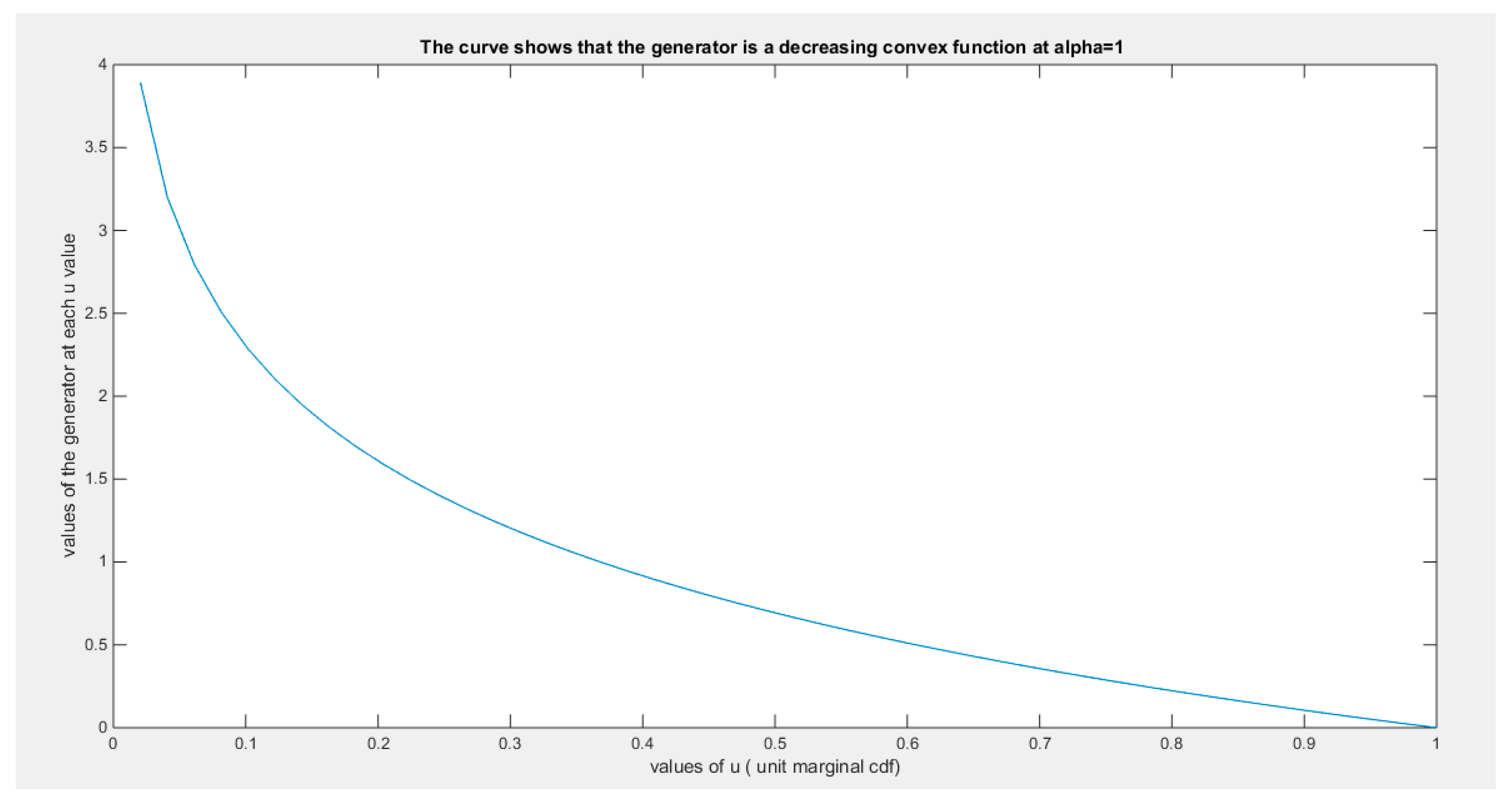
Figure 9. shows the joint CDF copula (copula) at alpha=0.1.

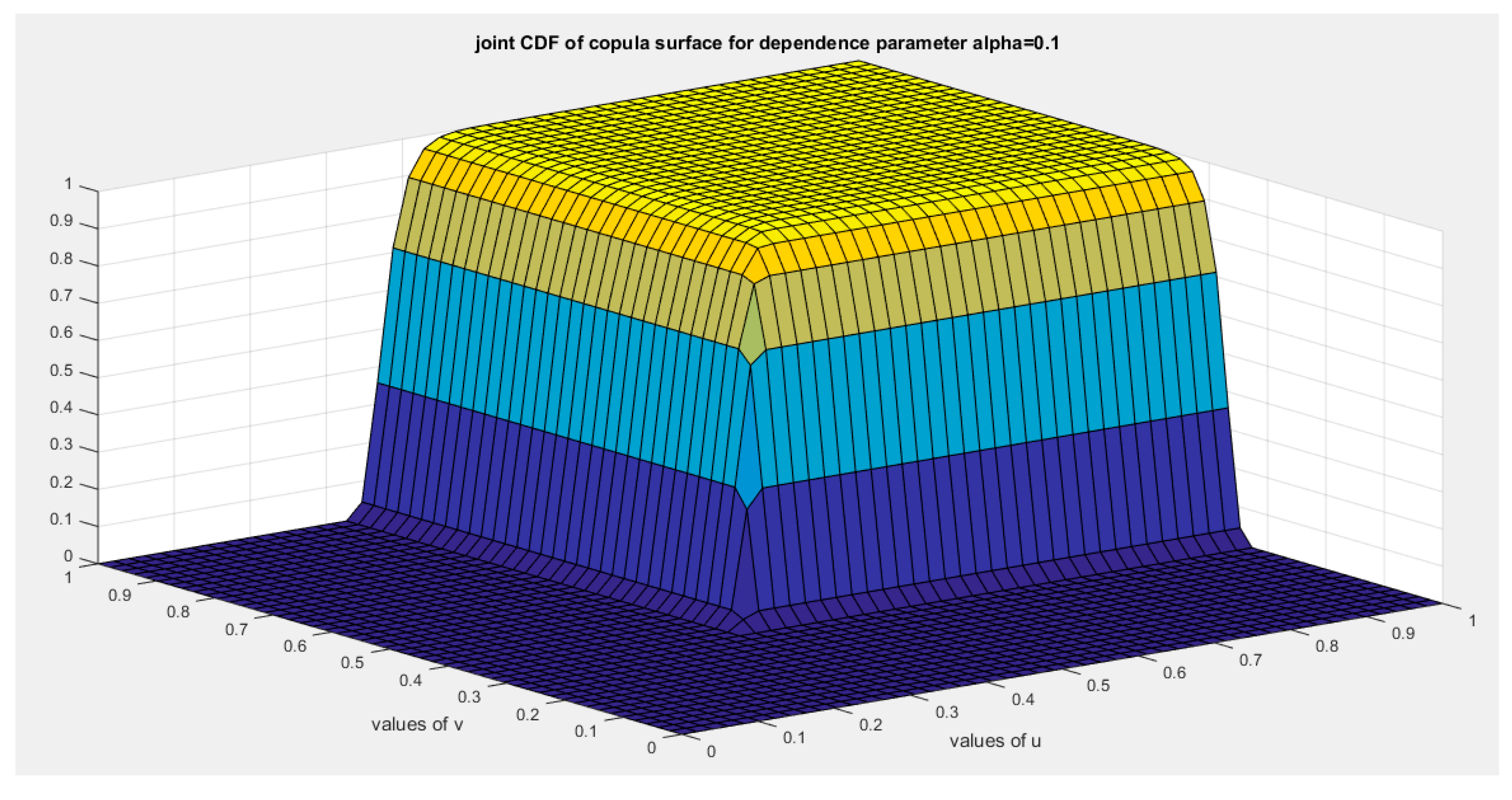
Figure 10. shows the joint PDF copula (copula density) at alpha =0.1.

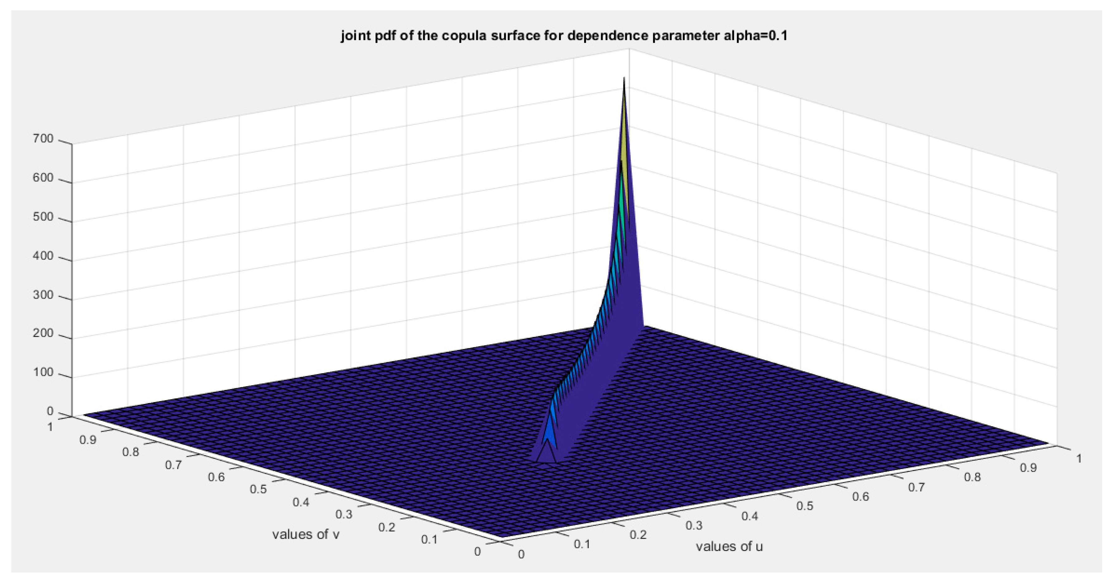
Figure 11. shows the joint CDF copula (copula) at alpha =0.4.

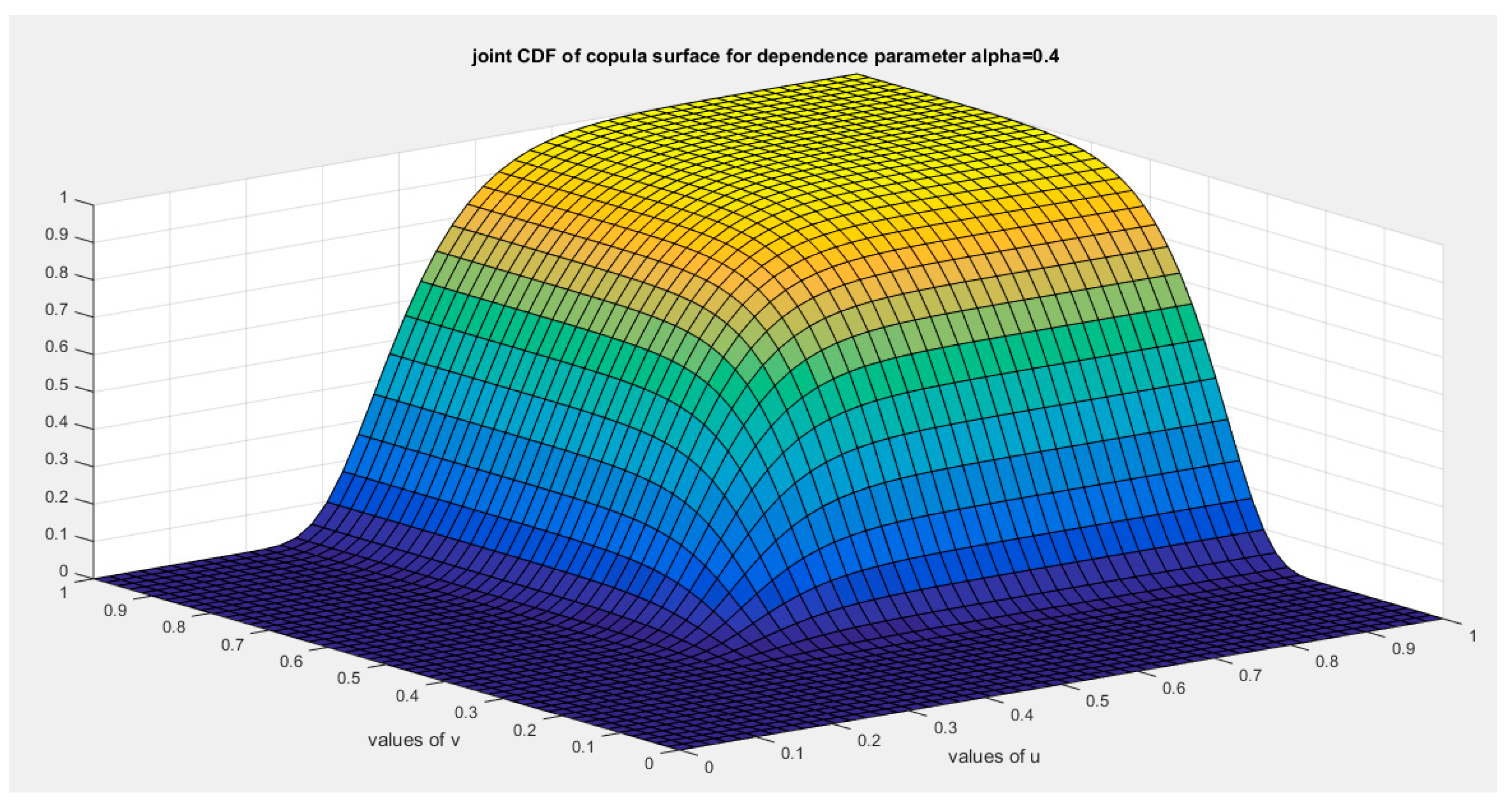
Figure 12. shows the joint PDF copula (copula density) at alpha =0.4.

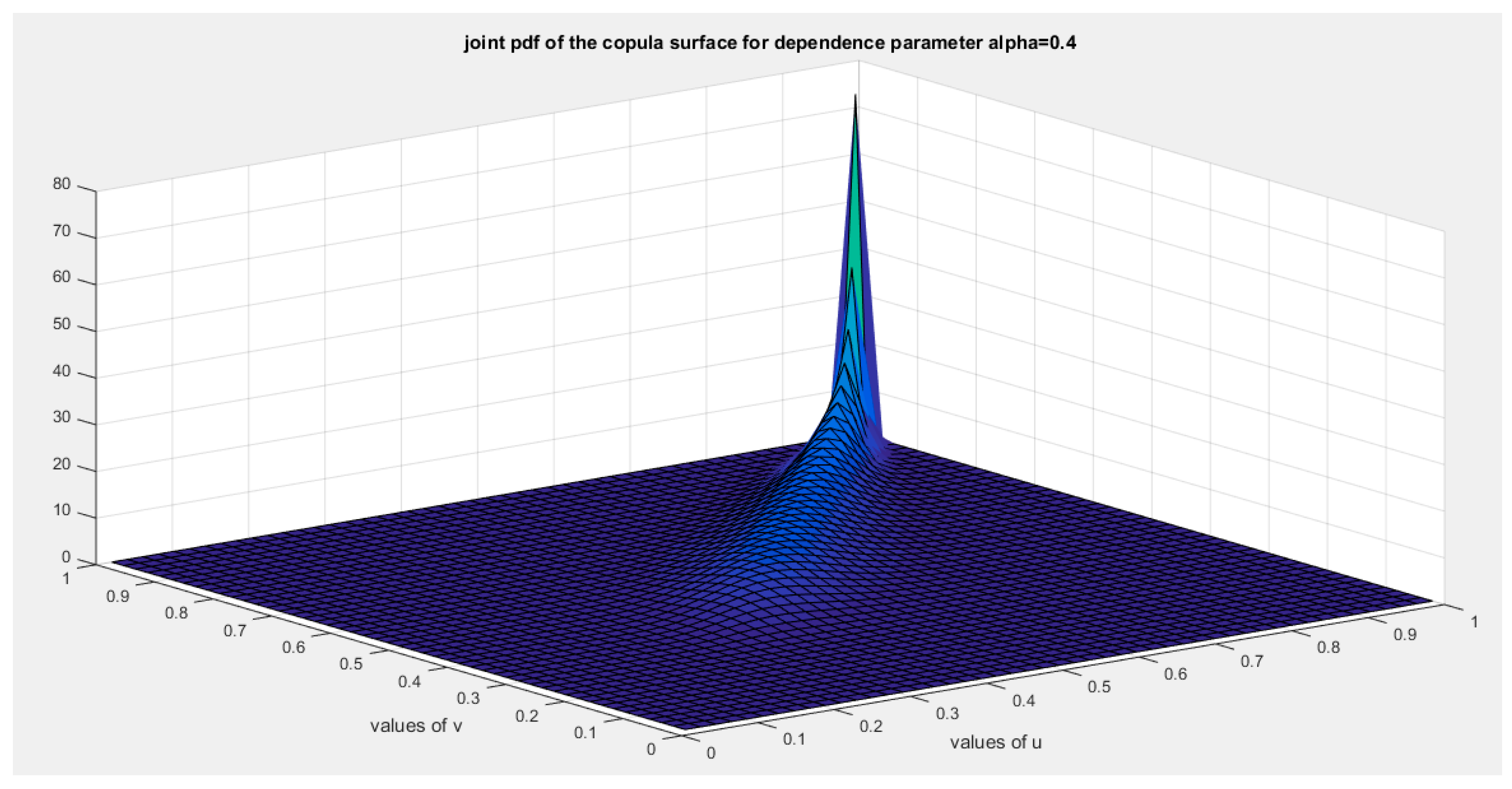
Figure 13. shows the joint CDF copula (copula) at alpha =0.6.

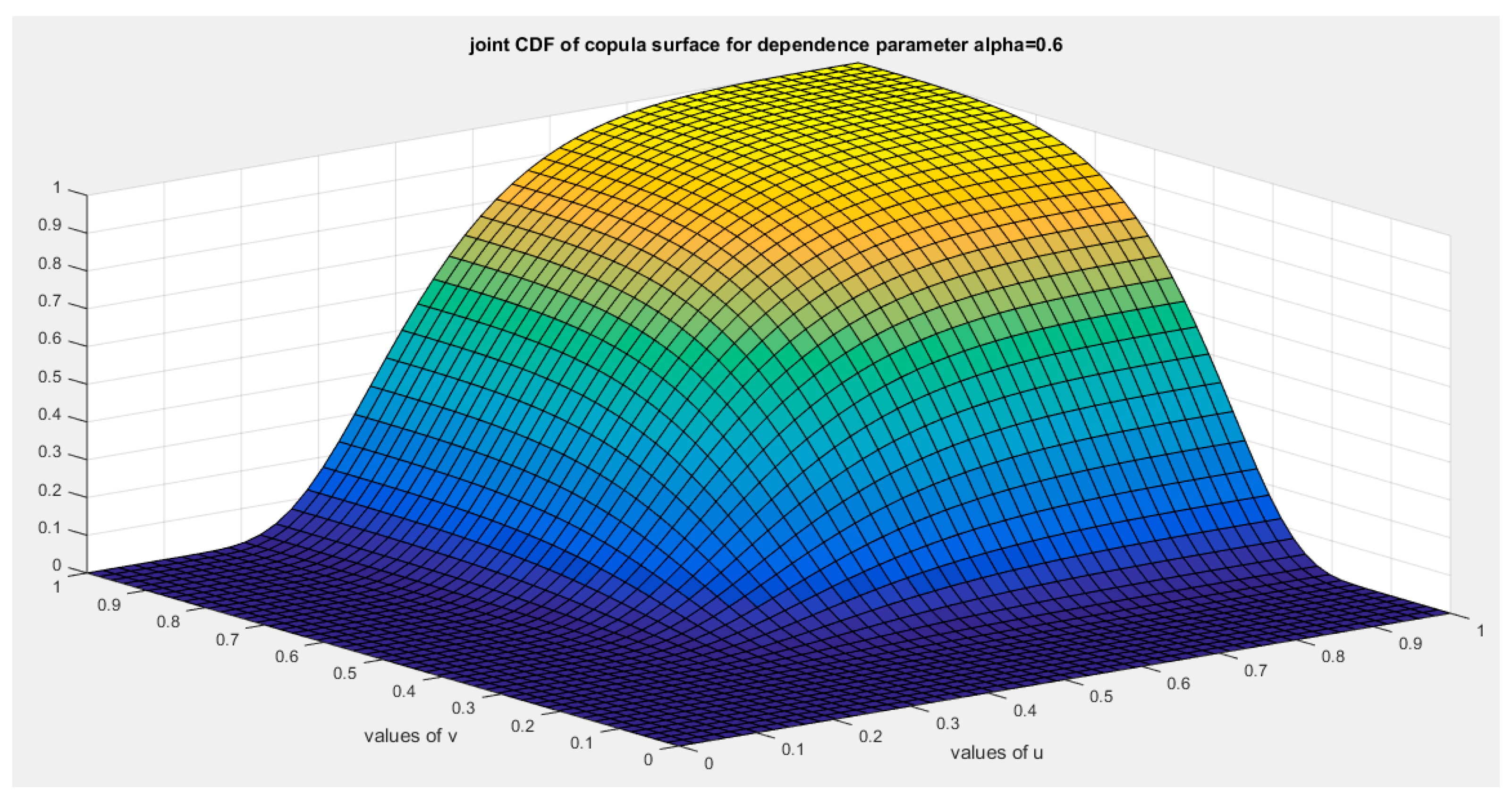
Figure 14. shows the joint PDF copula (copula density) at alpha =0.6.

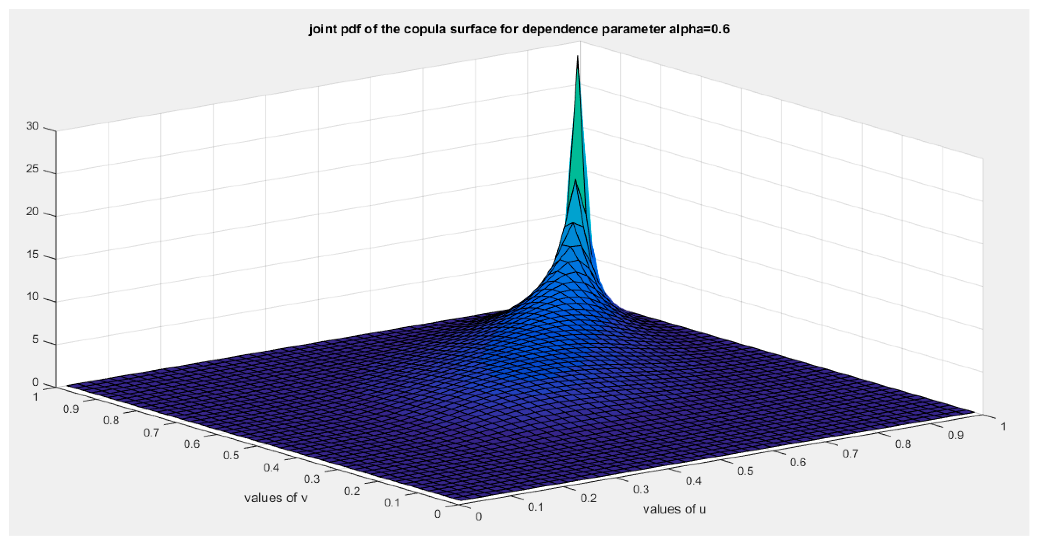
Figure 15. shows the joint CDF copula (copula) at alpha =0.888.

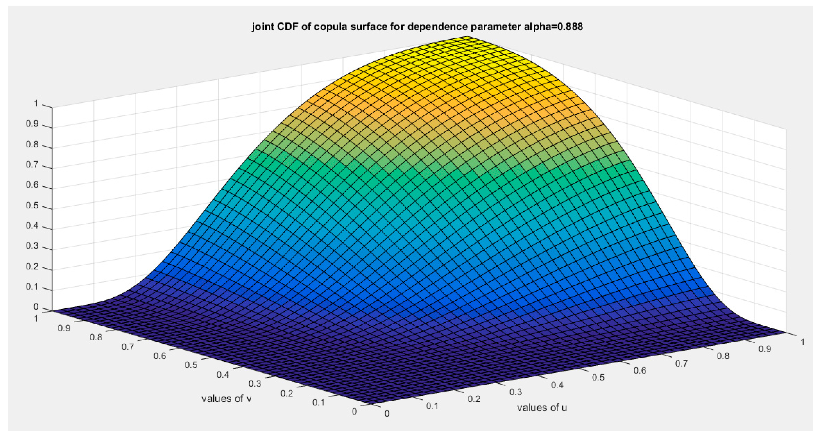
Figure 16. shows the joint PDF copula (copula density) at alpha =0.888.

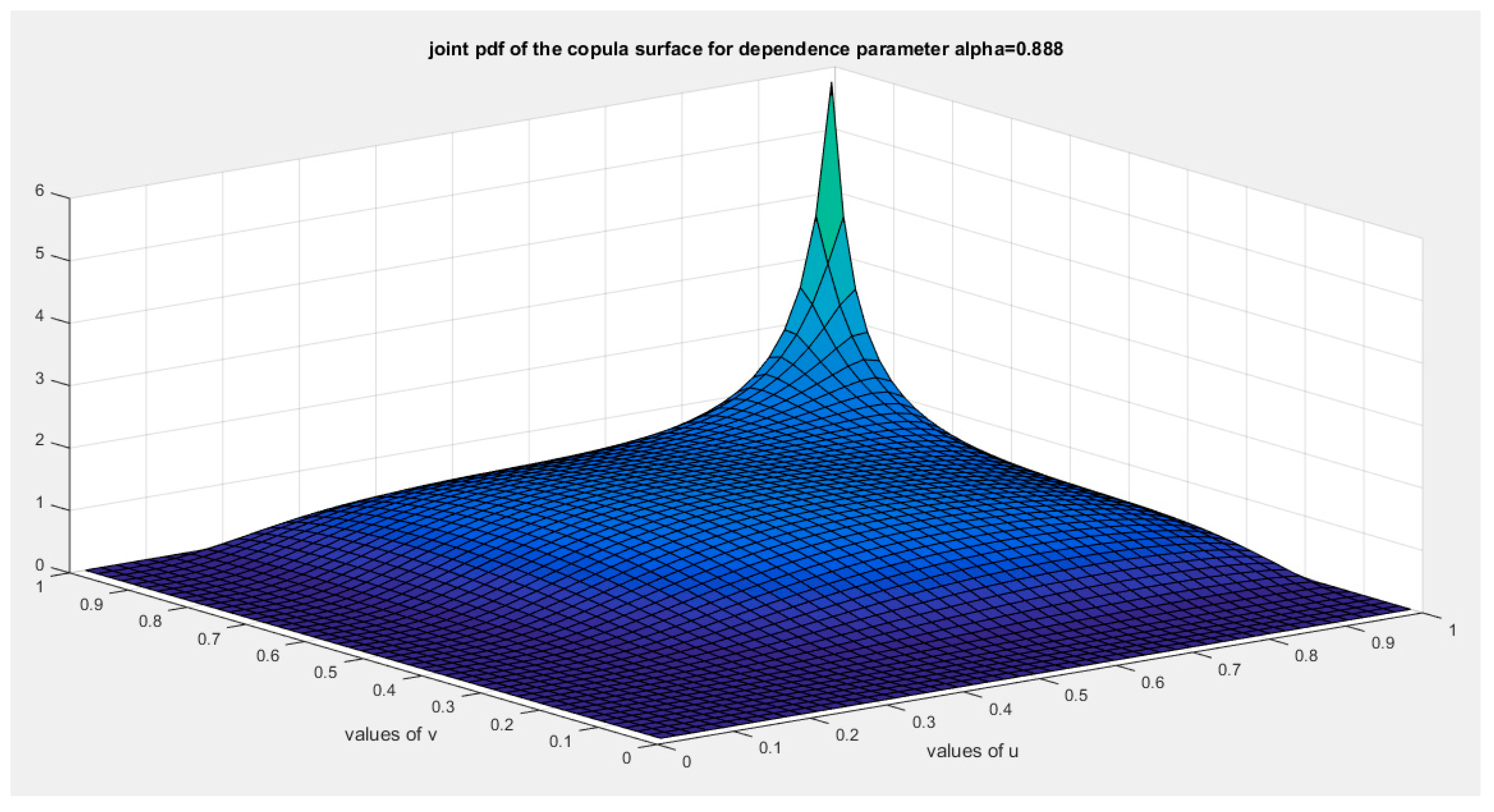
Figure 17. shows the joint CDF copula (copula) at alpha =0.988.

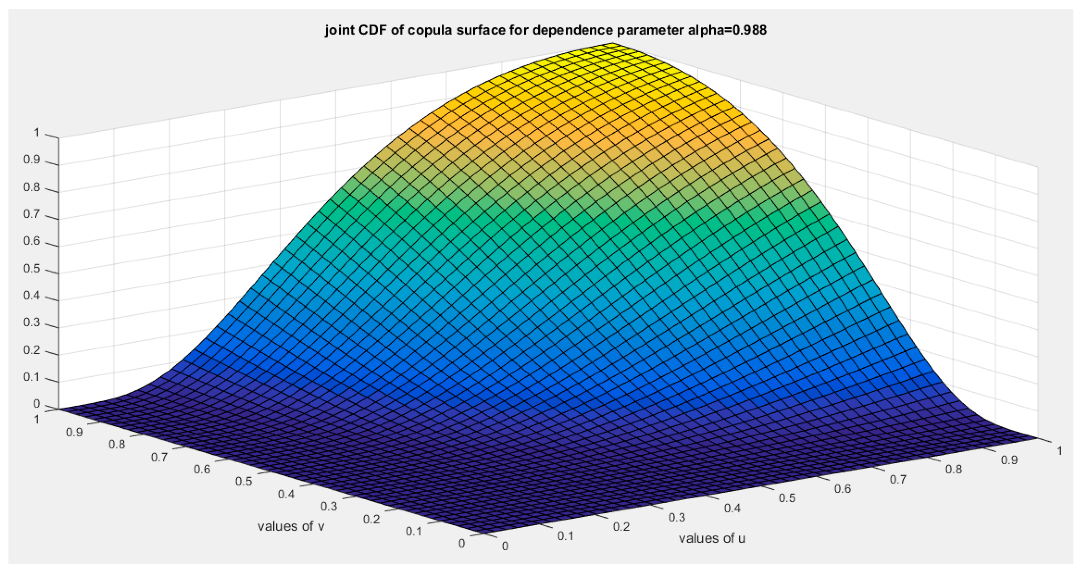
Figure 18. shows the joint PDF copula (copula density) at alpha =0.988.

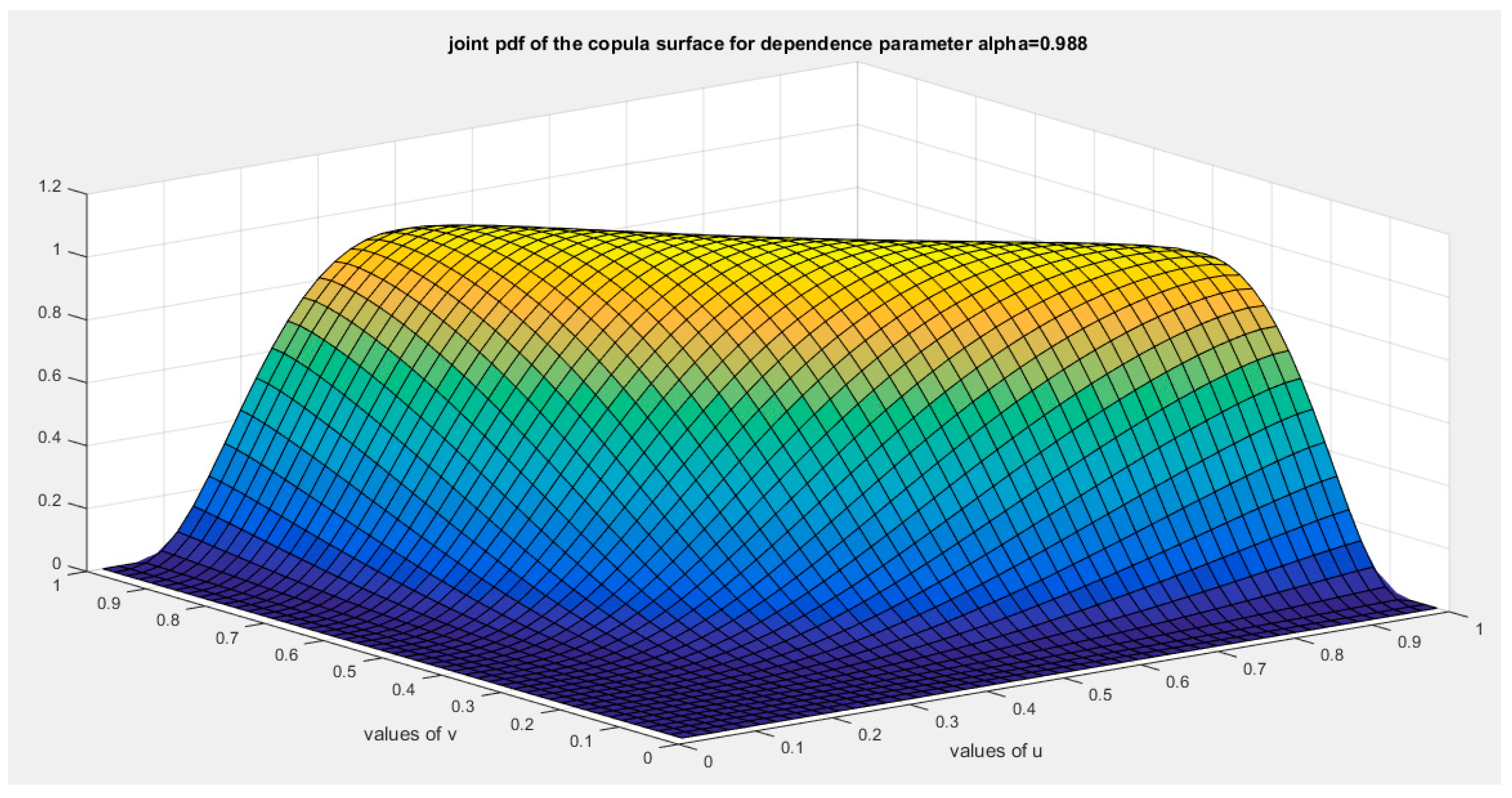
Figure 19. shows the joint CDF copula (copula) at alpha =1.

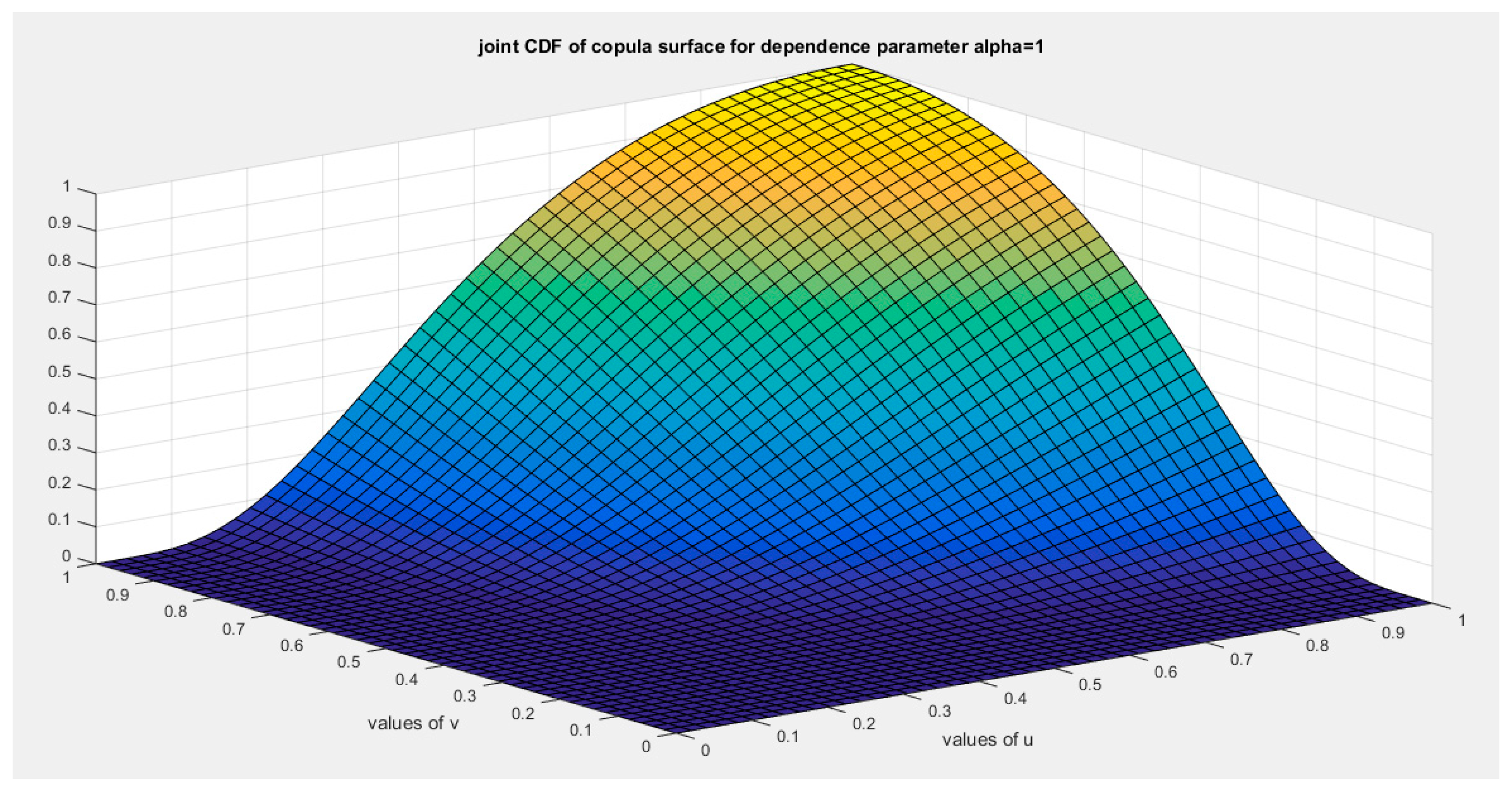
Figure 20. shows the joint PDF copula (copula density) at alpha =1.

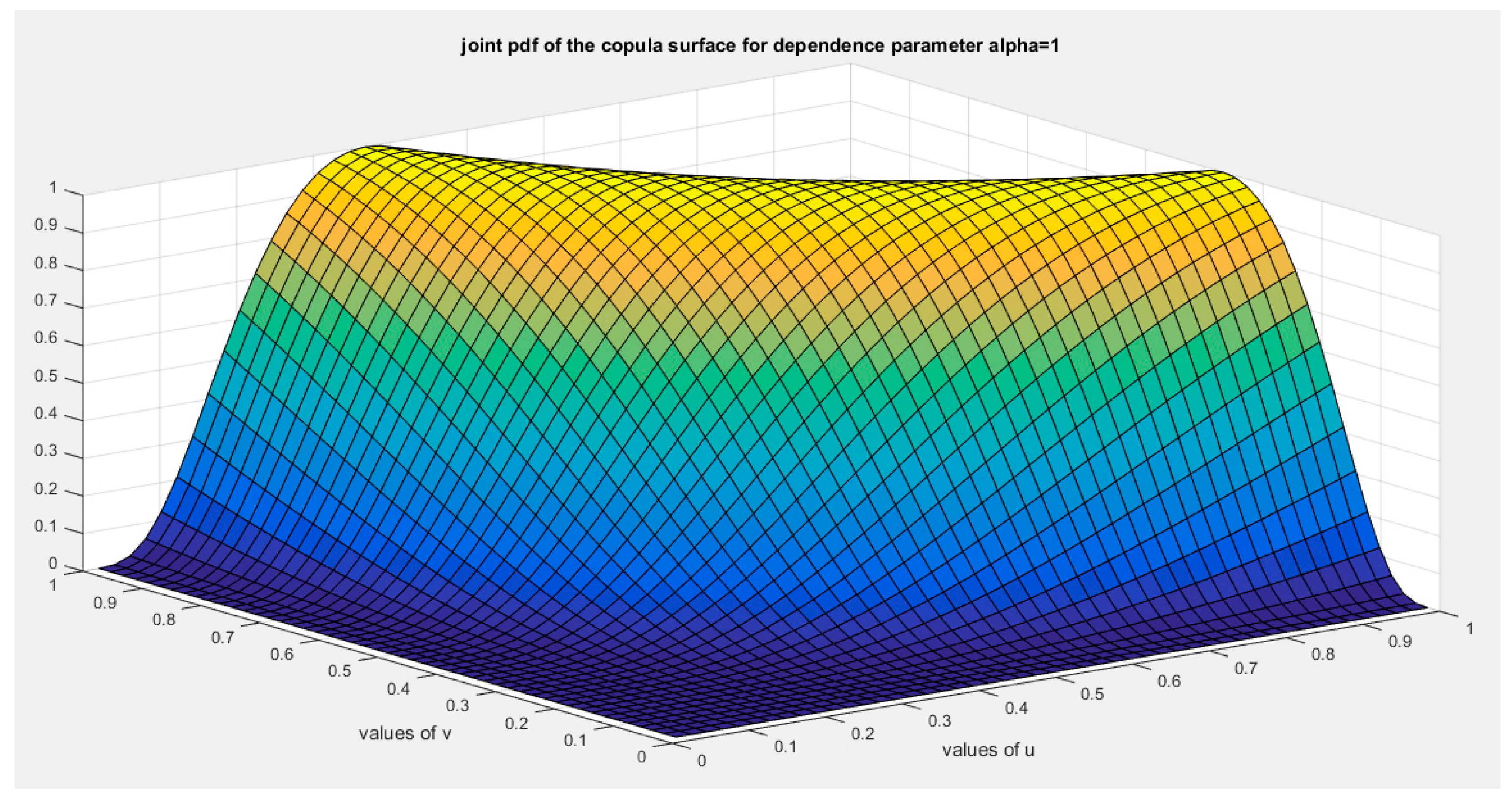
The limitation of this copula it does not cover independency.

Section 3: (Third Copula)

This copula depends on the frailty method for generating the copula. Assuming two individuals have survival time distributed as exponential

T_{1}

and

T_{2}

.They have exponential baseline hazard function with

λ_{1} = λ_{2} = 1

. The survival function is shown in equation (2) and the hazard function in equation ()

S (t) = P r o b (T > t) = 1 - F (t) \dots \dots \dots .

(2)

h (t) = - \frac{\partial \ln S (t)}{\partial t} = \frac{F (t)}{S (t)}

The Cox proportional hazard model uses the hazard function as shown in equation (3)

h (t, Z) = e^{β Z} b (t) \dots \dots \dots . .

(3)

where the Z are the explanatory variables in survival analysis and b(t) is the baseline hazard function. And B is the vector of regression coefficients. It is proportional because all information is contained in the multiplicative factor

γ = e^{B Z}

, this is called the frailty model when some explanatory variables (Z) and hence the factor

γ

are unobserved. And the factor

γ

is called the frailty parameter. Integrating and exponentiating the negative hazard

λ = e^{β_{0} + β_{1} Z_{1} + β_{2} Z_{2}} = e^{β_{0}} e^{β_{1} Z_{1} + β_{2} Z_{2}} = λ_{0} e^{β_{1} Z_{1} + β_{2} Z_{2}}

for 2 explanatory variables for example

S (t | γ) = e x p (- \int_{0}^{t} - \frac{\partial \ln S (t)}{\partial t}) d t = e x p (- \int_{0}^{t} h (t)) d t = e x p (- \int_{0}^{t} λ) d t e x p (- \int_{0}^{t} e^{β_{0} + β_{1} Z_{1} + β_{2} Z_{2}}) d t = e x p (- \int_{0}^{t} e^{β_{0} γ}) d t = e x p (- γ \int_{0}^{t} e^{β_{0}}) d t e^{(- γ \int_{0}^{t} e^{β_{0}} d t)} = {[e^{(- \int_{0}^{t} λ_{0} d t)}]}^{γ} = {[e^{- t λ_{0}}]}^{γ} w h e r e e^{β_{0}} = λ_{0} a s s u m e λ_{0} = 1

{[B (t)]}^{γ} w h e r e B (t) i s t h e b a s e l i n e h a z a r d

, to sum up

{[e^{- t λ_{0}}]}^{γ} = {[e^{- S_{0 (t)}}]}^{γ} = e^{- t γ} = S (t | γ)

The marginal distribution for a single life time T is obtained by taking expectation over the potential values of

γ

that is

E (e^{- t γ})

, assuming the

f (γ)

is the PDF of the frailty variable so

E (e^{- t γ}) = \int_{0}^{\infty} e^{- t γ} f (γ) d γ

Let y be a random variable distributed as Median Based Unit Rayleigh (BMUR)in equation (4) previously introduced by Iman Attia (Iman M. Attia, 2024), transform this variable to be defined on the interval from zero to infinity as shown below:

\frac{6}{α^{2}} [1 - y^{\frac{1}{α^{2}}}] y^{(\frac{2}{α^{2}} - 1)}, 0 < y < 1, α > 0

Let

w = - \ln {(y)}^{\frac{1}{α^{3}}} \to w = \frac{- \ln y}{α^{3}} \to - w α^{3} = \ln y \to y = e^{- α^{3} w}

d y = e^{- α^{3} w} (- α^{3}) d w \int_{0}^{\infty} \frac{6}{α^{2}} [1 - {(e^{- α^{3} w})}^{\frac{1}{α^{2}}}] {(e^{- α^{3} w})}^{(\frac{2}{α^{2}})} {(e^{- α^{3} w})}^{- 1} (α^{3}) e^{- α^{3} w} d w \int_{0}^{\infty} 6 α [1 - e^{- \frac{α^{3} w}{α^{2}}}] e^{- \frac{2 α^{3} w}{α^{2}}} d w f_{W} (w) = 6 α [1 - e^{- w α}] e^{- 2 α w}

Now this w is the frailty variable

γ

which is distributed as unbounded MBUR defined on the interval

(0, \infty)

.

E (e^{- t γ}) = \int_{0}^{\infty} e^{- t γ} f (γ) d γ = \int_{0}^{\infty} (e^{- t γ}) 6 α [1 - e^{- γ α}] e^{- 2 α γ} d γ = 6 α \int_{0}^{\infty} e^{- γ (t + 2 α)} d γ - 6 α \int_{0}^{\infty} e^{- γ (t + 3 α)} d γ = 6 α {[\frac{e^{- γ (t + 2 α)}}{- (t + 2 α)}]|}_{0}^{\infty} - 6 α {[\frac{e^{- γ (t + 3 α)}}{- (t + 3 α)}]|}_{0}^{\infty} = 6 α [(\frac{1}{t + 2 α}) - (\frac{1}{t + 3 α})] = E (e^{- t γ}) = E (S (t | γ)) = \frac{6 α^{2}}{(t + 2 α) (t + 3 α)} = \frac{6 α^{2}}{t^{2} + 5 α t + 6 α^{2}}

We can think of this expectation as a function of the frailty variable, it is averaging the probability to survive beyond specific time given that frailty. It is the expectation of a function of the frailty not the variable frailty itself so this function which is the baseline survival function should be multiplied by the PDF of the frailty variable. This way the frailty variable is integrated out. So this expectation is considered as the joint CDF of the two random variables T1 and T2. How to get this time? By inverting this expectation. Let us call this expectation u then solving second degree polynomial to get its root.

(u = \frac{6 α^{2}}{t^{2} + 5 α t + 6 α^{2}}) \to (\frac{6 α^{2}}{u} = t^{2} + 5 α t + 6 α^{2}) \to (t^{2} + 5 α t + 6 α^{2} - \frac{6 α^{2}}{u} = 0) t = \frac{- 5 α + \sqrt{25 α^{2} - 4 (1) (6 α^{2}) (1 - \frac{1}{u})}}{2} t = \frac{- 5 α + \sqrt{25 α^{2} - 24 α^{2} (1 - \frac{1}{u})}}{2} t = \frac{- 5 α + \sqrt{α^{2} (25 - 24 (1 - \frac{1}{u}))}}{2} = \frac{- 5 α + α \sqrt{(25 - 24 (1 - \frac{1}{u}))}}{2} t = \frac{α (- 5 + \sqrt{(25 - 24 + \frac{24}{u})})}{2} = \frac{α (- 5 + \sqrt{(1 + \frac{24}{u})})}{2}

This (t) is the generator and (u) is the inverse generator. So the time (t) is a function of (u)

The generator should fulfill the sufficient conditions:

(1): $φ (0) = \frac{α (- 5 + \sqrt{(1 + \frac{24}{0})})}{2} = \infty$
(2): $φ (1) = \frac{α (- 5 + \sqrt{(1 + \frac{24}{1})})}{2} = 0$
(3): $φ^{'} (u) = \frac{α}{4} {(1 + \frac{24}{u})}^{- 0.5} (\frac{- 24}{u^{2}}) = - 6 α {(1 + \frac{24}{u})}^{- 0.5} (\frac{1}{u^{2}}) < 0$

This ensures that the generator is a decreasing function.
(4): $φ^{''} (u) = \frac{12 α}{u^{3}} {(1 + \frac{24}{u})}^{- 0.5} + \frac{6 α}{2} {(1 + \frac{24}{u})}^{- 1.5} (\frac{- 24}{u^{2}}) (\frac{1}{u^{2}}) > 0$ $= \frac{12 α}{u^{3}} {(1 + \frac{24}{u})}^{- 0.5} - \frac{72 α}{u^{4}} {(1 + \frac{24}{u})}^{- 1.5} > 0 f o r α > 0$

This ensures that the generator is convex at

0 < α \leq 1

for bivariate distribution:

φ (u) = \frac{α (- 5 + \sqrt{(1 + \frac{24}{u})})}{2}, t h i s i s t h e g e n e r a t o r φ (v) = \frac{α (- 5 + \sqrt{(1 + \frac{24}{v})})}{2} φ (w) = φ (u) + φ (v) = \frac{α (- 5 + \sqrt{(1 + \frac{24}{u})})}{2} + \frac{α (- 5 + \sqrt{(1 + \frac{24}{v})})}{2} φ (w) = \frac{α}{2} \{- 10 + \sqrt{(1 + \frac{24}{u})} + \sqrt{(1 + \frac{24}{v})}\} C (φ (u) + φ (v)) = 6 α^{2} {({[φ (w)]}^{2} + 5 α [φ (w)] + 6 α^{2})}^{- 1} C (u, v) = C (F_{X} (x), F_{Y} (y))

For a copula to be a valid copula it should fulfill the boundary condition, the marginal uniformity and 2- increasing conditions. And this is equivalent for necessary conditions of the inverse generator to be fulfilled which are the following:

Proposition 10

: The boundary conditions and marginal uniformity:

C (0, v) = C (u, 0) = 0

, boundary condition.

C (1, v) = v a n d C (u, 1) = u

, the marginal uniformity.

Proof:

when u=1 so :

φ (w) = \frac{α}{2} \{- 10 + \sqrt{(1 + \frac{24}{1})} + \sqrt{(1 + \frac{24}{v})}\} = = \frac{α}{2} \{- 5 + \sqrt{(1 + \frac{24}{v})}\} C (1, v) = \frac{6 α^{2}}{(φ (w) + 2 α) (φ (w) + 3 α)} C (1, v) = \frac{6 α^{2}}{(\frac{α}{2} \{- 5 + \sqrt{(1 + \frac{24}{v})}\} + 2 α) (\frac{α}{2} \{- 5 + \sqrt{(1 + \frac{24}{v})}\} + 3 α)} C (1, v) = \frac{6 α^{2}}{(\frac{α}{2} \{- 5 + \sqrt{(1 + \frac{24}{v})}\} + \frac{4 α}{2}) (\frac{α}{2} \{- 5 + \sqrt{(1 + \frac{24}{v})}\} + \frac{6 α}{2})} C (1, v) = \frac{6 α^{2}}{(\frac{α}{2} (\{- 5 + \sqrt{(1 + \frac{24}{v})}\} + 4)) (\frac{α}{2} (\{- 5 + \sqrt{(1 + \frac{24}{v})}\} + 6))} C (1, v) = \frac{6 α^{2}}{(\frac{α}{2} [- 1 + \sqrt{(1 + \frac{24}{v})}]) (\frac{α}{2} [1 + \sqrt{(1 + \frac{24}{v})}])} C (1, v) = \frac{6 α^{2}}{(\frac{α^{2}}{4}) [- 1 + \sqrt{(1 + \frac{24}{v})} - \sqrt{(1 + \frac{24}{v})} + (1 + \frac{24}{v})]} C (1, v) = \frac{24}{[(\frac{24}{v})]} = v

The same is true for v , if v=1 so

C (u, 1) = \frac{24}{[(\frac{24}{u})]} = u

Proposition 11

: for copula to be valid it should be 2-increasing in other words

\frac{\partial^{2} C (u, v)}{\partial u \partial v} \geq 0 \frac{\partial C (u, v)}{\partial u} = - 6 α^{2} {[{(φ (w))}^{2} + 5 α φ (w) + 6 α^{2}]}^{- 2} [2 \{φ (w)\} (\frac{α}{2}) (\frac{1}{2}) {(1 + \frac{24}{u})}^{- 0.5} (\frac{- 24}{u^{2}})] + 5 α (\frac{α}{2}) (\frac{1}{2}) {(1 + \frac{24}{u})}^{- 0.5} (\frac{- 24}{u^{2}}) = \frac{36 α^{4}}{u^{2}} {(1 + \frac{24}{u})}^{- 0.5} \{- 5 + {(1 + \frac{24}{u})}^{0.5} + {(1 + \frac{24}{u})}^{0.5}\} {[{(φ (w))}^{2} + 5 α φ (w) + 6 α^{2}]}^{- 2} \frac{\partial}{\partial v} (\frac{\partial C (u, v)}{\partial u}) = \frac{(432) α^{4}}{u^{2} v^{2}} {(1 + \frac{24}{u})}^{- 0.5} {(1 + \frac{24}{v})}^{- 0.5} {[{(φ (w))}^{2} + 5 α φ (w) + 6 α^{2}]}^{- 2} \times \{α^{2} {[{(φ (w))}^{2} + 5 α φ (w) + 6 α^{2}]}^{- 1} {[- 5 + {(1 + \frac{24}{u})}^{0.5} + {(1 + \frac{24}{u})}^{0.5}]}^{2} - 1\}

Proposition 12

: this copula is absolutely continuous copula and it has no singular part.

Proof:

to test for singularity:

\frac{φ (0)}{φ^{'} (0)} = 0

φ (u) = \frac{α}{2} (- 5 + {(1 + \frac{24}{u})}^{0.5}) \frac{φ (u)}{φ^{'} (u)} = \frac{\frac{α}{2} (- 5 + {(1 + \frac{24}{u})}^{0.5})}{(\frac{α}{2}) (\frac{1}{2}) {(1 + \frac{24}{u})}^{- 0.5} (\frac{- 24}{u^{2}})} = \frac{(- 5 + {(1 + \frac{24}{u})}^{0.5})}{(\frac{1}{2}) {(1 + \frac{24}{u})}^{- 0.5} (\frac{- 24}{u^{2}})} \lim_{u \to 0} \frac{φ (u)}{φ^{'} (u)} = \underset{u \to 0}{l i m} \frac{(- 5 + {(1 + \frac{24}{u})}^{0.5})}{(\frac{1}{2}) {(1 + \frac{24}{u})}^{- 0.5} (\frac{- 24}{u^{2}})} = \underset{u \to 0}{l i m} \frac{- 5}{(\frac{1}{2}) {(1 + \frac{24}{u})}^{- 0.5} (\frac{- 24}{u^{2}})} + \underset{u \to 0}{l i m} \frac{{(1 + \frac{24}{u})}^{0.5}}{(\frac{1}{2}) {(1 + \frac{24}{u})}^{- 0.5} (\frac{- 24}{u^{2}})} = \underset{u \to 0}{l i m} \frac{- 10}{{(1 + \frac{24}{u})}^{- 0.5} (\frac{- 24}{u^{2}})} + \underset{u \to 0}{l i m} \frac{(1 + \frac{24}{u})}{(\frac{- 12}{u^{2}})} = \underset{u \to 0}{l i m} \frac{- 10}{{(\frac{u}{u} + \frac{24}{u})}^{- 0.5} (\frac{- 24}{u^{2}})} + \underset{u \to 0}{l i m} \frac{(1 + \frac{24}{u})}{(\frac{- 12}{u^{2}})} \underset{u \to 0}{l i m} \frac{- 10}{{(\frac{u}{u + 24})}^{0.5} (\frac{- 24}{u^{2}})} + \underset{u \to 0}{l i m} \frac{(\frac{24 + u}{u}) u^{2}}{- 12} \underset{u \to 0}{l i m} \frac{- 10 {(u + 24)}^{0.5} u^{2}}{- 24 u^{0.5}} + \underset{u \to 0}{l i m} \frac{u (24 + u)}{- 12} \underset{u \to 0}{l i m} \frac{10 {(u + 24)}^{0.5} u^{1.5}}{24} + \underset{u \to 0}{l i m} \frac{u (24 + u)}{- 12} = 0 + 0 = 0

As long as this limit is zero at u=0 so the copula has no singular part and it is absolutely continuous copula.

Proposition 13

: Kendall tau for this copula is τ = 1 − 2α²

Proof:

τ = 4 \int_{0}^{1} \frac{φ (u)}{φ^{'} (u)} d u + 1 \int_{0}^{1} \frac{φ (u)}{φ^{'} (u)} d u = \int_{0}^{1} (\frac{10 {(u + 24)}^{0.5} u^{1.5}}{24} + \frac{u (24 + u)}{- 12}) d u = = \frac{10}{24} \int_{0}^{1} {(u + 24)}^{0.5} u^{1.5} d u + \frac{- 1}{12} \int_{0}^{1} 24 u + u^{2} d u = = \frac{10}{24} (0.8286) - \frac{1}{12} (12 + \frac{1}{3}) = - 0.19917 τ = 4 \int_{0}^{1} \frac{φ (u)}{φ^{'} (u)} d u + 1 = 4 (- 0.19917) + 1 = 0.20332

The following figures show the generator and the CDF and PDF of this third copula

Figure 21. shows the generator function (decreasing and convex) at alpha = 0.1.

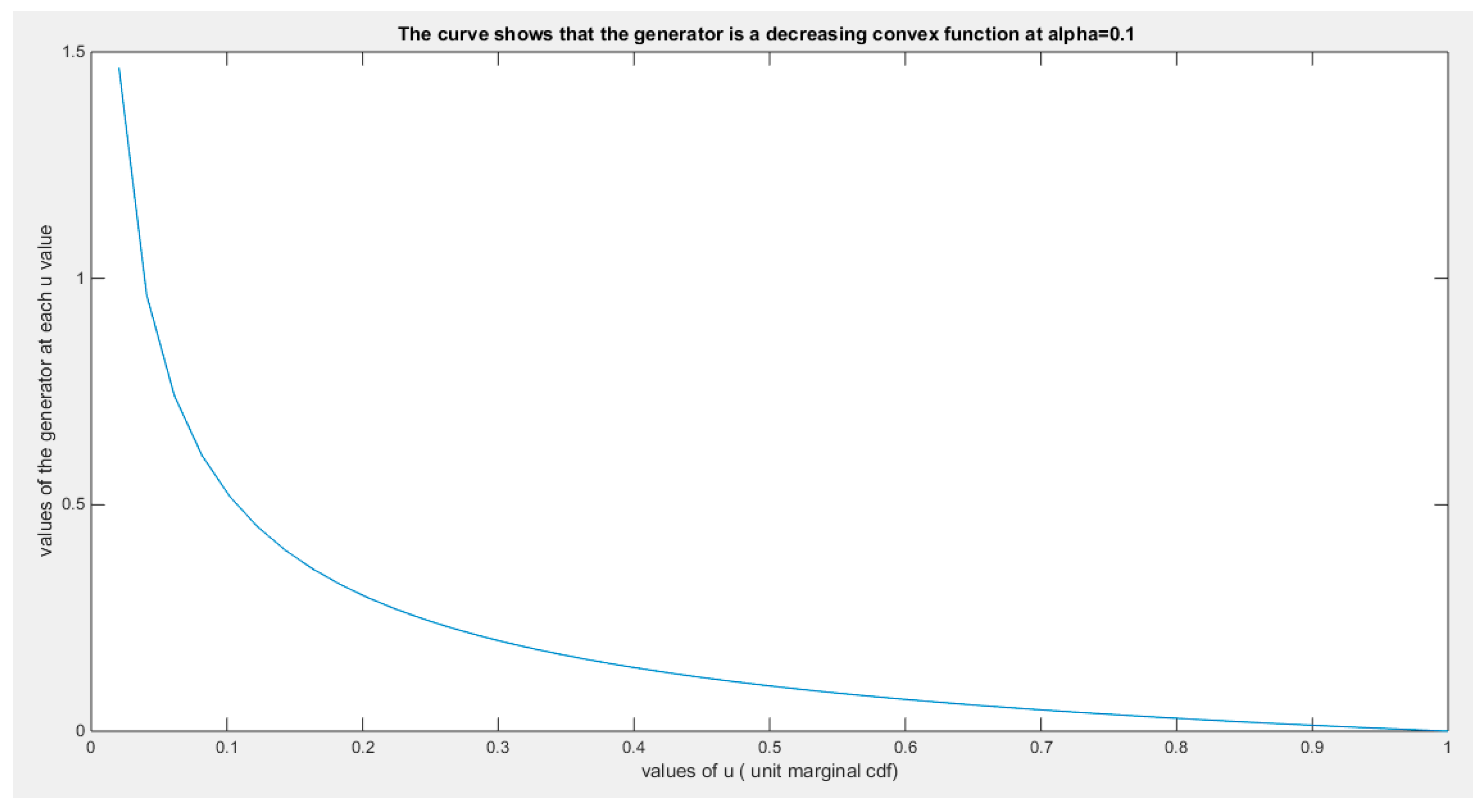
Figure 22. shows the joint CDF copula (copula density) at alpha =0.1.

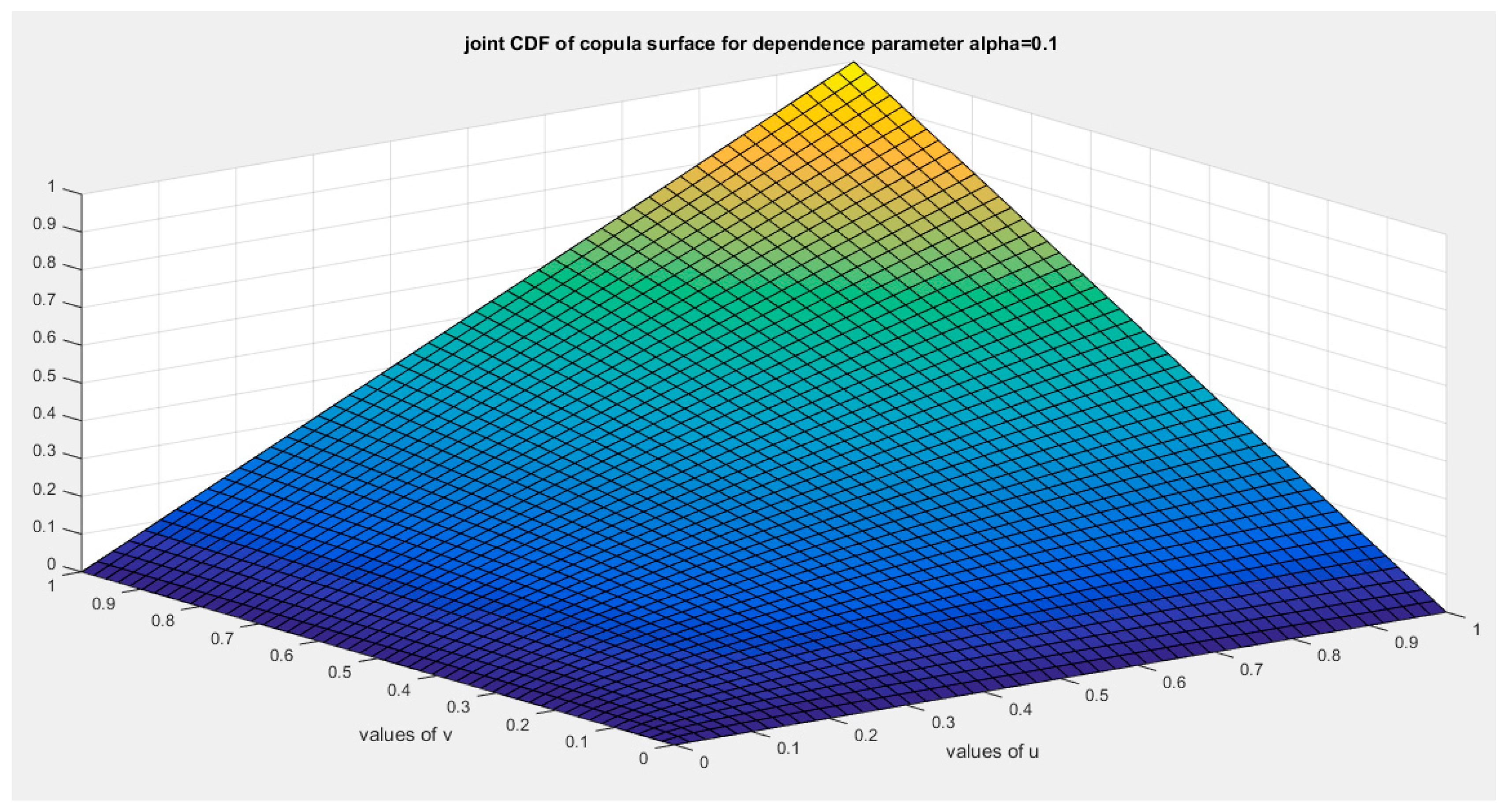
Figure 23. shows the joint PDF copula (copula density) at alpha =0.1.

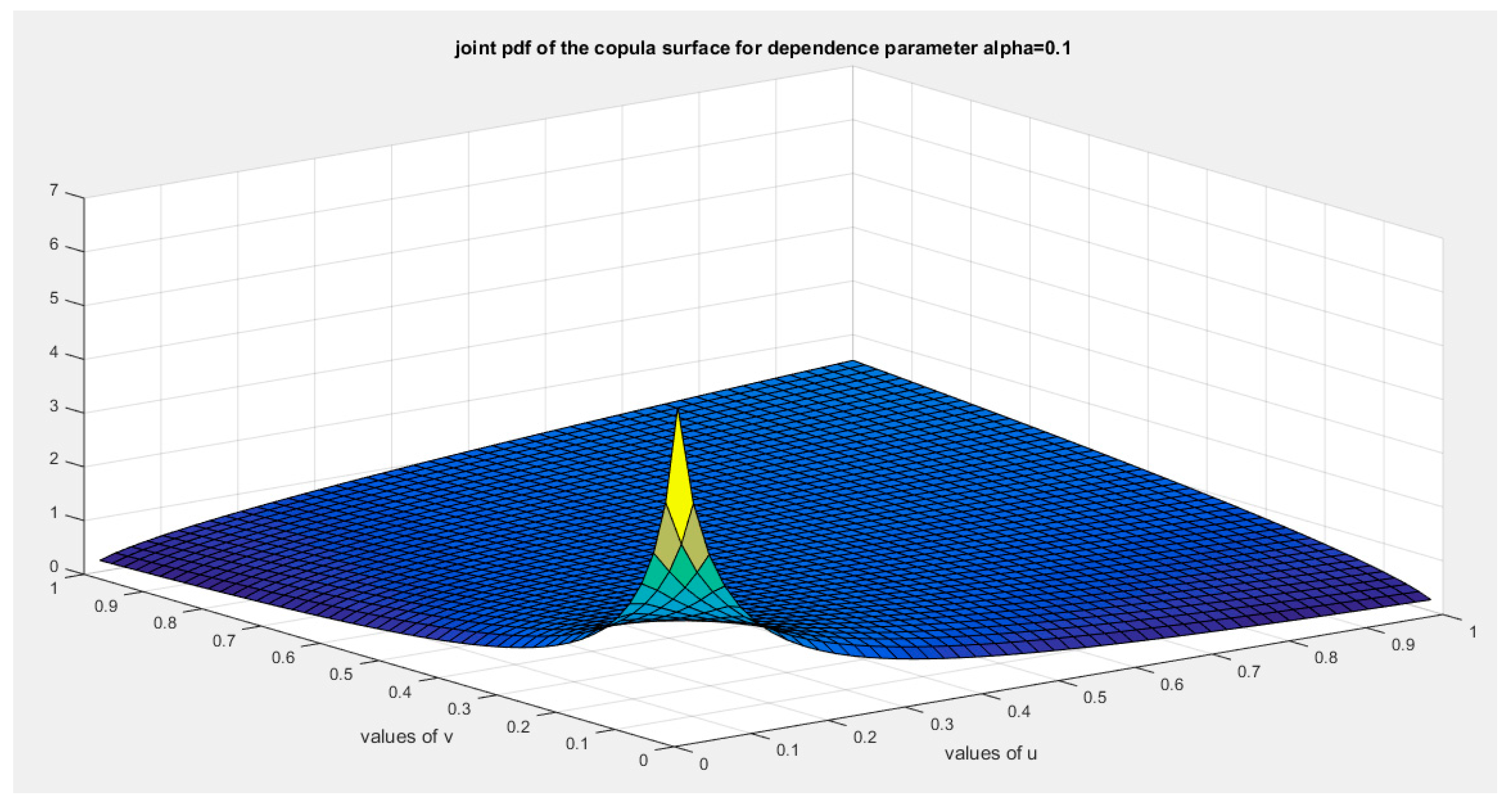
Figure 23. shows the joint CDF copula (copula) at alpha =0.6.

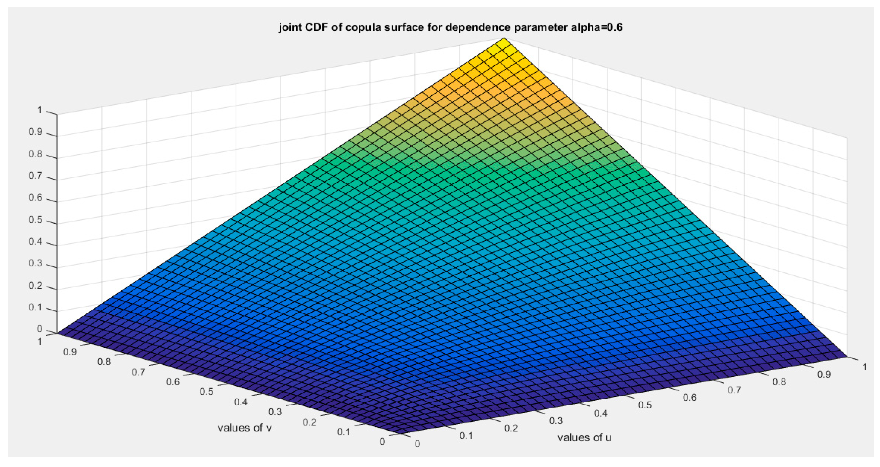
Figure 24. shows the joint PDF copula (copula density) at alpha =0.6.

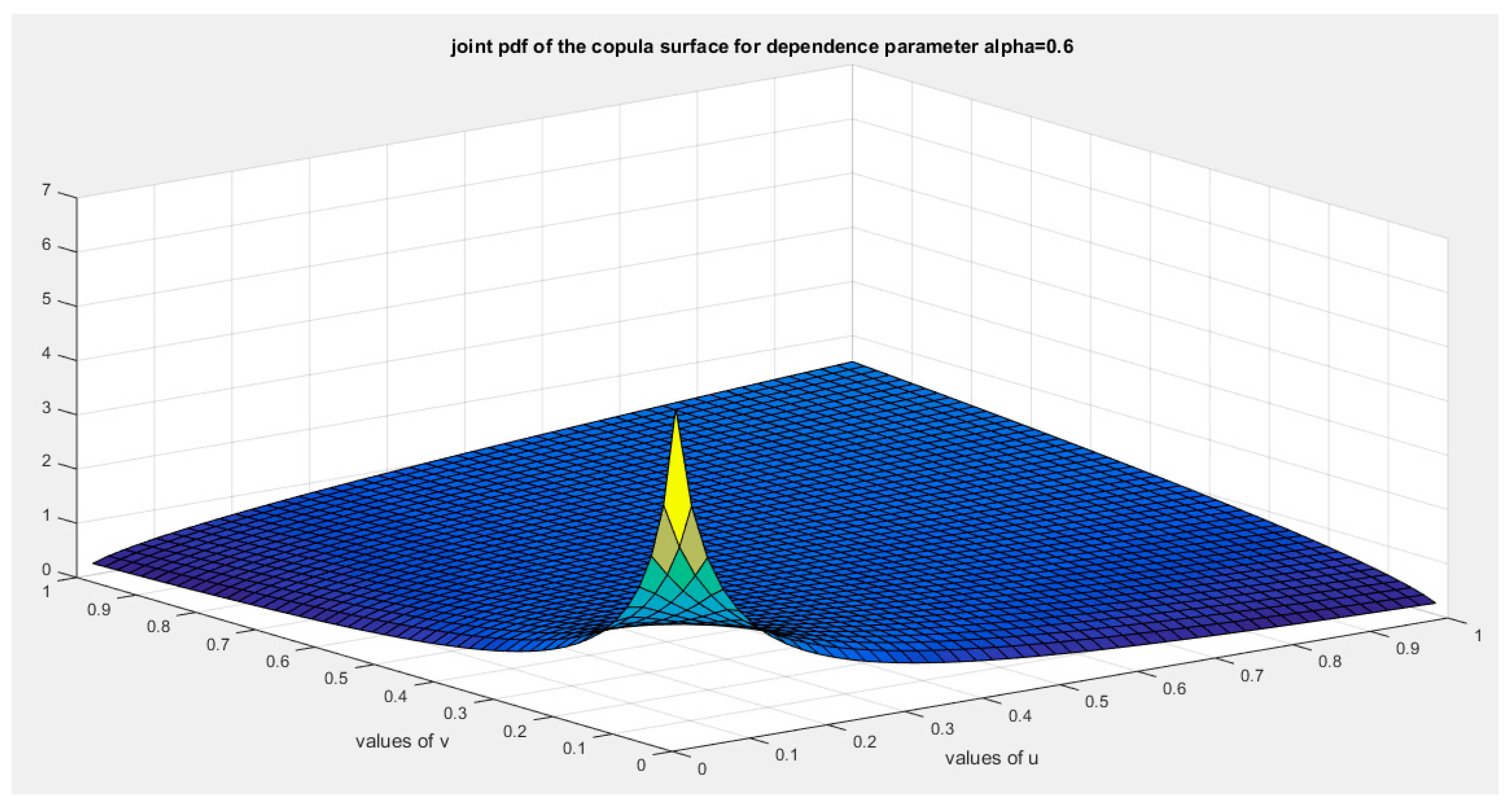
Figure 25. shows the joint CDF copula (copula) at alpha =1.

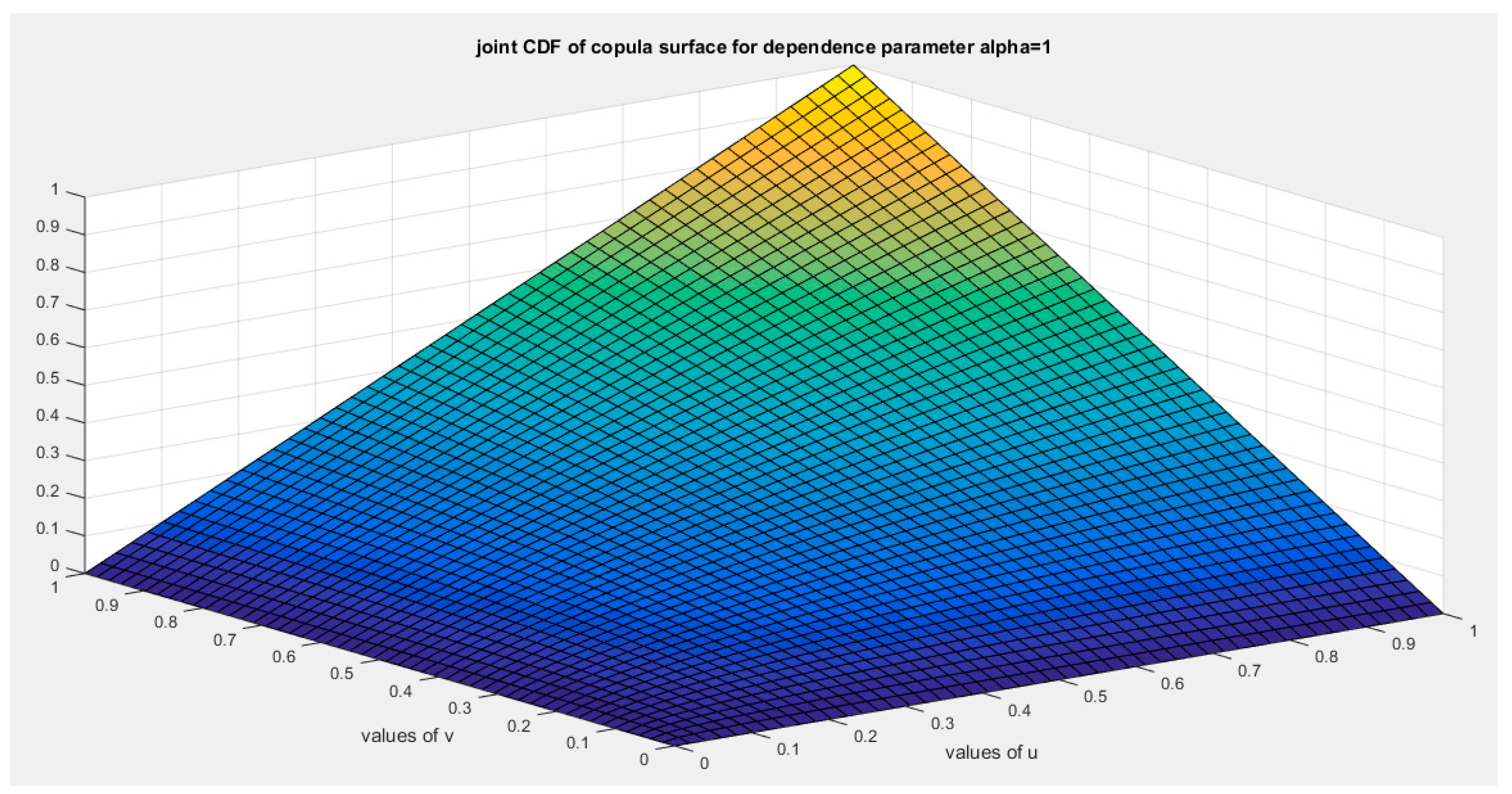
Figure 26. shows the joint PDF copula (copula density) at alpha =1.

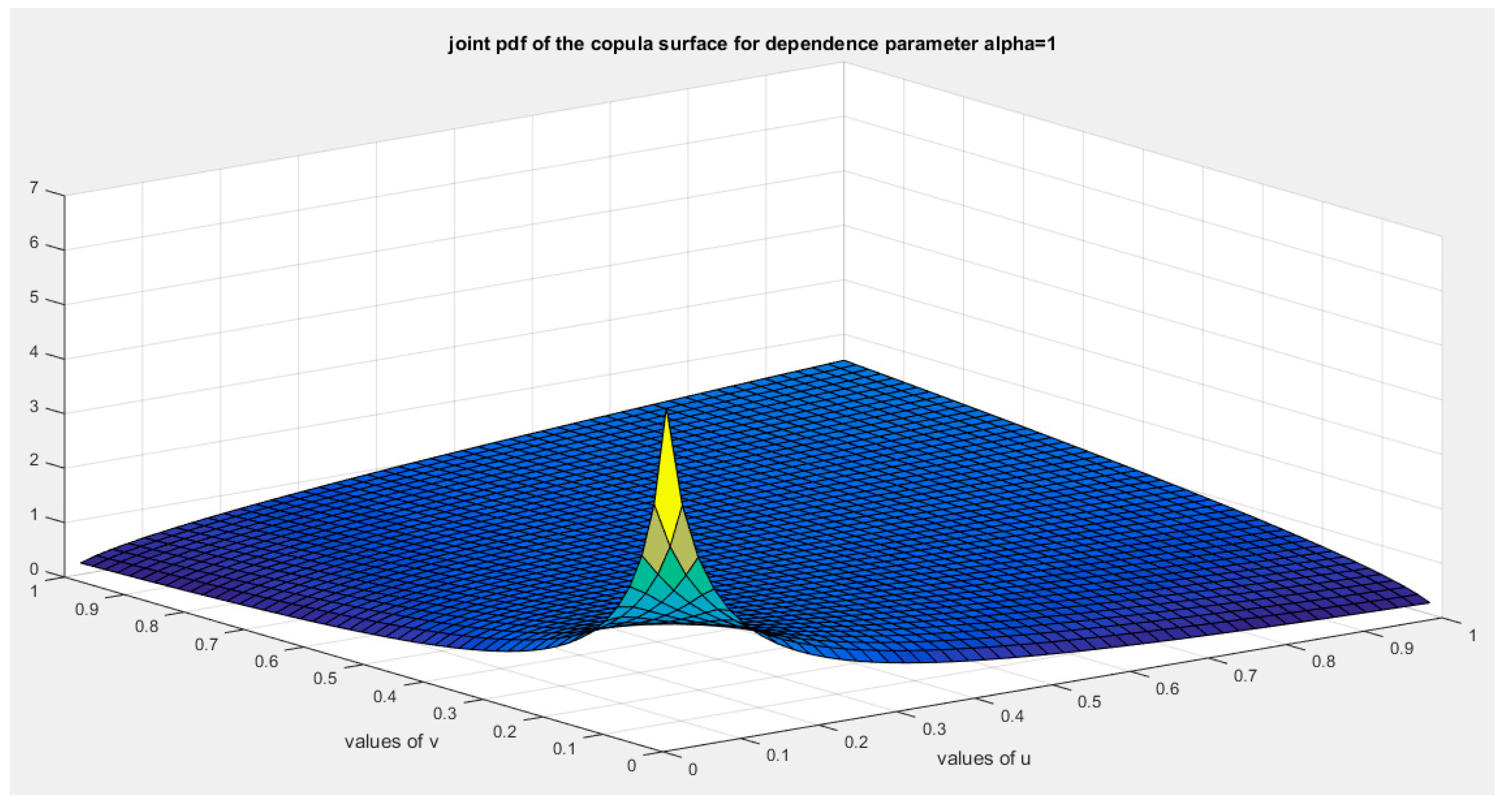
Figure 27. shows the joint CDF copula (copula) at alpha =10.

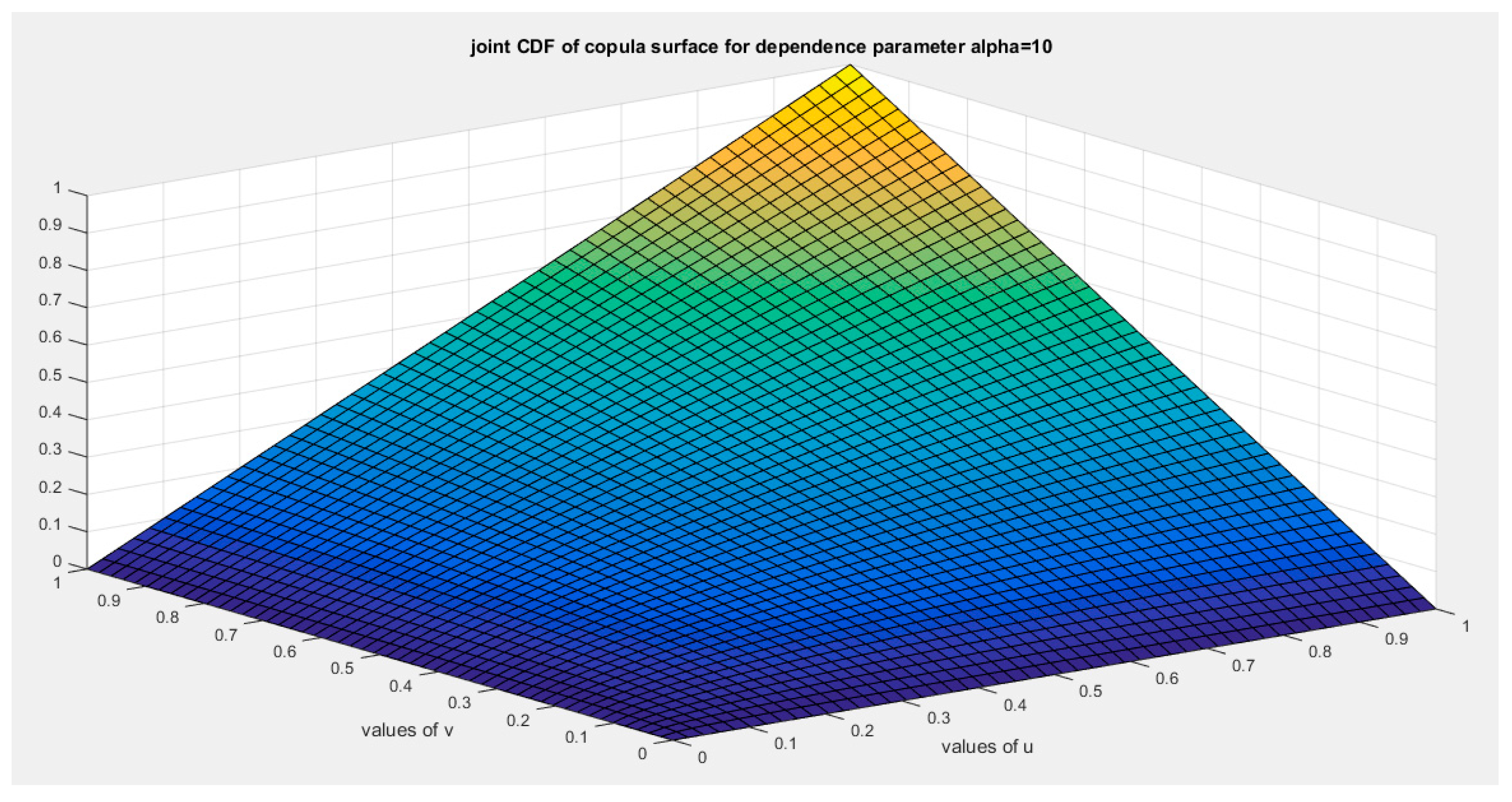
Figure 28. shows the joint PDF copula (copula density) at alpha =1.

To sum up for this copula, the generator and inverse generator fulfill the conditions. The copula density fulfills the criteria but the values of the joint CDF and DPF are the same for all values of the dependency parameter. Kendal tau is fixed at 0.32 and it does not depend on the dependency parameter.

Section 4: Conclusions and Future Work

Although the generator and inverse generator fulfilled the criteria as well as the copula density but for each copula discussed previously, there were limitations. These limitation may be solved by mixture of copulas or better re-parameterization of these copula once again.

Declarations:

Ethics Approval and Consent to Participate

Not applicable.

Consent for publication

Not applicable

Availability of Data and Material

Not applicable. Data sharing not applicable to this article as no datasets were generated or analyzed during the current study.

Competing Interests

The author declares no competing interests of any type.

Funding

No funding resource. No funding roles in the design of the study and collection, analysis, and interpretation of data and in writing the manuscript are declared.

Authors’ Contribution

AI carried the conceptualization by formulating the goals, aims of the research article, formal analysis by applying the statistical, mathematical and computational techniques to synthesize and analyze the hypothetical data, carried the methodology by creating the model, software programming and implementation, supervision, writing, drafting, editing, preparation, and creation of the presenting work.

References

Abe Sklar. Random Variables, Joint distribution functions, and copulas. Kybernetika 1973, 9, 449–460. [Google Scholar]
Bhat, C. R. , & Eluru, N. A copula-based approach to accommodate residential self-selection effects in travel behavior modeling. Transportation Research Part B: Methodological 2009, 43, 749–765. [Google Scholar] [CrossRef]
De Lira Salvatierra, I. , & Patton, A. J. Dynamic copula models and high frequency data. Journal of Empirical Finance 2015, 30, 120–135. [Google Scholar] [CrossRef]
Dokuzoğlu, D. , & Purutçuoğlu, V. Comprehensive Analyses of Gaussian Graphical Model under Different Biological Networks. Acta Physica Polonica A 2017, 132, 1106–1111. [Google Scholar] [CrossRef]
Genest, C. , & Mackay, J. The Joy of Copulas: Bivariate Distributions with Uniform Marginals. The American Statistician 1986, 40, 280–283. [Google Scholar] [CrossRef]
Gomes, M. , Radice, R., Camarena Brenes, J., & Marra, G. Copula selection models for non-Gaussian outcomes that are missing not at random. Statistics in Medicine 2019, 38, 480–496. [Google Scholar] [CrossRef] [PubMed]
Iman, M. Attia. A Novel Unit Distribution Named asMedian Based Unit Rayleigh (MBUR):Properties and Estimations. Preprints.Org, 7 October. [CrossRef]
Kilgore, R. T. , & Thompson, D. B. Estimating Joint Flow Probabilities at Stream Confluences by Using Copulas. Transportation Research Record: Journal of the Transportation Research Board 2011, 2262, 200–206. [Google Scholar] [CrossRef]
Kole, E. , Koedijk, K., & Verbeek, M. Selecting copulas for risk management. Journal of Banking & Finance 2007, 31, 2405–2423. [Google Scholar] [CrossRef]
Konigorski, S. , Yilmaz, Y. E., & Bull, S. B. Bivariate genetic association analysis of systolic and diastolic blood pressure by copula models. BMC Proceedings 2014, 8, S72. [Google Scholar] [CrossRef]
Kuss, O. , Hoyer, A., & Solms, A. Meta-analysis for diagnostic accuracy studies: A new statistical model using beta-binomial distributions and bivariate copulas. Statistics in Medicine 2014, 33, 17–30. [Google Scholar] [CrossRef] [PubMed]
Lapuyade-Lahorgue, J. , Xue, J.-H., & Ruan, S. Segmenting Multi-Source Images Using Hidden Markov Fields With Copula-Based Multivariate Statistical Distributions. IEEE Transactions on Image Processing 2017, 26, 3187–3195. [Google Scholar] [CrossRef] [PubMed]
Liu, Z. , Guo, S., Xiong, L., & Xu, C.-Y. Hydrological uncertainty processor based on a copula function. Hydrological Sciences Journal 2018, 63, 74–86. [Google Scholar] [CrossRef]
Ma, X. , Luan, S., Du, B., & Yu, B. Spatial Copula Model for Imputing Traffic Flow Data from Remote Microwave Sensors. Sensors 2017, 17, 2160. [Google Scholar] [CrossRef]
Oh, D. H. , & Patton, A. J. Time-Varying Systemic Risk: Evidence From a Dynamic Copula Model of CDS Spreads. Journal of Business & Economic Statistics 2018, 36, 181–195. [Google Scholar] [CrossRef]
Oppenheimer, M. , Little, C. M., & Cooke, R. M. Expert judgement and uncertainty quantification for climate change. Nature Climate Change 2016, 6, 445–451. [Google Scholar] [CrossRef]
Salvadori, G., Michele, C. D., Kottegoda, N. T., & Rosso, R. (2007). Extremes in Nature: An Approach Using Copulas (Vol. 56). Springer Netherlands. [CrossRef]
Schölzel, C. , & Friederichs, P. Multivariate non-normally distributed random variables in climate research – introduction to the copula approach. Nonlinear Processes in Geophysics 2008, 15, 761–772. [Google Scholar] [CrossRef]
Valle, D. , & Kaplan, D. Quantifying the impacts of dams on riverine hydrology under non-stationary conditions using incomplete data and Gaussian copula models. Science of The Total Environment 2019, 677, 599–611. [Google Scholar] [CrossRef] [PubMed]

Disclaimer/Publisher’s Note: The statements, opinions and data contained in all publications are solely those of the individual author(s) and contributor(s) and not of MDPI and/or the editor(s). MDPI and/or the editor(s) disclaim responsibility for any injury to people or property resulting from any ideas, methods, instructions or products referred to in the content.

© 2025 by the authors. Licensee MDPI, Basel, Switzerland. This article is an open access article distributed under the terms and conditions of the Creative Commons Attribution (CC BY) license (http://creativecommons.org/licenses/by/4.0/).

Copyright: This open access article is published under a Creative Commons CC BY 4.0 license, which permit the free download, distribution, and reuse, provided that the author and preprint are cited in any reuse.

New Three Different Generators for Constructing New Three Different Bivariate Copulas

Abstract

Keywords:

Subject:

Introduction

Section 1: (First Copula)

Section 2: (Second Copula)

Section 3: (Third Copula)

Section 4: Conclusions and Future Work

Declarations:

Ethics Approval and Consent to Participate

Consent for publication

Availability of Data and Material

Competing Interests

Funding

Authors’ Contribution

References

MDPI Initiatives

Important Links

Subscribe