Submitted:
16 April 2025
Posted:
17 April 2025
You are already at the latest version
Abstract
In the paper we suggest an algorithm of fuzzy clustering with uninorm-based distance measure. The algorithm follows a general scheme of fuzzy c-means (FCM) clustering, but in contrast to the existing algorithm it implements logical distance between data instances. The centers of the clusters calculated by the algorithm are less deviated and are concentrated in the areas of the actual centers of the clusters that results in more accurate recognition of the number of clusters and of data structure.
Keywords:
fuzzy c‐means clustering
; uninorm
; absorbing norm
MSC: 62A86; 62H30; 91C20
1. Introduction
In general, decision making starts with formulation of possible alternatives, collecting required data, data analysis, formulation of the decision criteria and choice of the alternatives based on the formulated criteria [1].
In simple cases of decision making with certain information and univariate data, decision making process is reduced to the choice of alternatives which minimize the payoff or maximize the reward. In cases of uncertain information, decision making is more complicated and deals with the expected payoffs and rewards using probabilistic or other methods for handling uncertainty. Finally, in cases of multivariate data and multicriteria choices, decision making is hardly solvable by exact methods and can be considered as a kind of art.
For example, Triantaphyllou in his book [2] describes several methods of multicriteria decision making without suggesting any preferred technique and indicates that each specific decision-making problem requires specific method for its solution. Such an approach is supported by the authors of the book [3] who stress “a growing need for methodologies that, on the basis of the ever-increasing wealth of data available, are able to take into account all the relevant points of view, technically called criteria, and all the actors involved” [3] (p. ix) and then present classification of the methods for solving different decision-making problems.
To apply the methods of decision making the raw data are preprocessed with the aim of recognition of possible patterns and consequently – to decrease the number of instances and, if it is possible, the number of dimensions [4]. The basic preprocessing procedure which decreases the number of instances used in the next steps of decision making is data classification [5,6] or, if any additional information is unavailable – data clustering [7,8].
The popular clustering method is the k-means algorithm suggested independently by Lloyd [9] and by Forgy [10] and is known as Lloyd-Forgy algorithm. This algorithm obtains instances and creates clusters such that each instance is included into a single cluster for which Euclidean distance between the instance and the cluster’s center is minimal. The clusters are formed from the instances for which the within-cluster variances are also minimal. The FORTRAN implementation of the algorithm was published by Hartigan and Wong [11]. Currently, this algorithm is implemented in most statistical and mathematical software tools; for example, in MATLAB® it is implemented in the Statistics and Machine Learning Toolbox™ in the function kmeans [12].
Main disadvantage of the k-means algorithm and its direct successors is an inclusion of each instance only in a single cluster that often restricts recognition of the data patterns and interpretation of the obtained clusters.
To overcome this disadvantage Bezdek [13,14] suggested the fuzzy clustering algorithm widely known as the fuzzy c-means (FCM) algorithm. Following this algorithm, the clusters are considered as fuzzy sets, and each instance is included in several clusters with certain degrees of membership. In its original version, the algorithm uses Euclidean distances between the instances and the degrees of membership are calculated based on these distances. The other versions of the algorithm follow its original structure but use the other distance measures. For example, the Fuzzy Logic Toolbox™ of MATLAB® includes the function fcm [15], which implements the c-means algorithm with three distance measures: Euclidean distance, distance measure based on Mahalanobis distance from the instances and the cluster centers [16] and exponential distance measure normalized by the probability of choosing the cluster [17]. For the overview of different versions of the c-means algorithm and the other fuzzy clustering methods see the paper [18] and the book [19].
Along with the advantages of the fuzzy c-means clustering techniques, it inherits the following disadvantage of the k-means algorithm: both algorithms search for the predefined number of clusters and separate the cluster centers even in cases where such separation does not follow from the data structures. For example, if the data is a set of normally distributed instances, then it is expected that the clustering algorithm will recognize a single cluster, and the centers of all clusters will be placed close to the center of distribution. However, the c-means algorithm with the known distance measures does not provide such a result.
The suggested c-means algorithm with the uninorm-based distance solves this problem. Similar to the other fuzzy c-means algorithms, the suggested algorithm has the same structure as original Bezdek algorithm, but, in contrast to the known methods, it considers the normalized instances as truth values of certain propositions and implements fuzzy logical distance between them. The suggested distance is based on the probability-based uninorm and absorbing norm [22] which already demonstrated their usefulness in a wide range of decision-making and control tasks [23].
The suggested algorithm can be used for recognition of the patterns in raw data and for data preprocessing in different decision-making problems.
The rest of the paper is organized as follows. In section 2.1 we briefly outline the Bezdek fuzzy c-means algorithm and in section 2.2 describe the uninorm and absorbing norm which will be used for construction the logical distance. Section 3 presents the main results: the distance measure based on the uninorm and absorbing norm (section 3.1) and the resulting algorithm for fuzzy clustering (section 3.2). In section 3.3 we illustrate the activity of the algorithm by numerical simulations with different data distributions and compare the obtained results with the results provided by the known fuzzy c-means algorithms. Section 4 includes some discussable issues.
2. Materials and Methods
The suggested algorithm follows the structure of the Bezdek fuzzy c-means algorithm [13,14] but, in contrast to the existing algorithms, it uses the logical distance based on the uninorm and absorbing norm [20]. Below we briefly describe this algorithm and the used norms.
2.1. Fuzzy c-Means Algorithm
Assume that the raw data is given by -dimensional vectors of real numbers
where , , , , stands for the observation or instance of the data.
Given a number , denote by
a vector of the cluster centers, where , , , , denotes the center of the th cluster.
The problem is to define the centers of the clusters and to define the membership degree of each instance to each cluster .
The fuzzy c-means algorithm which solves this problem is outlined as follows [13] (see also [14,15,17]).
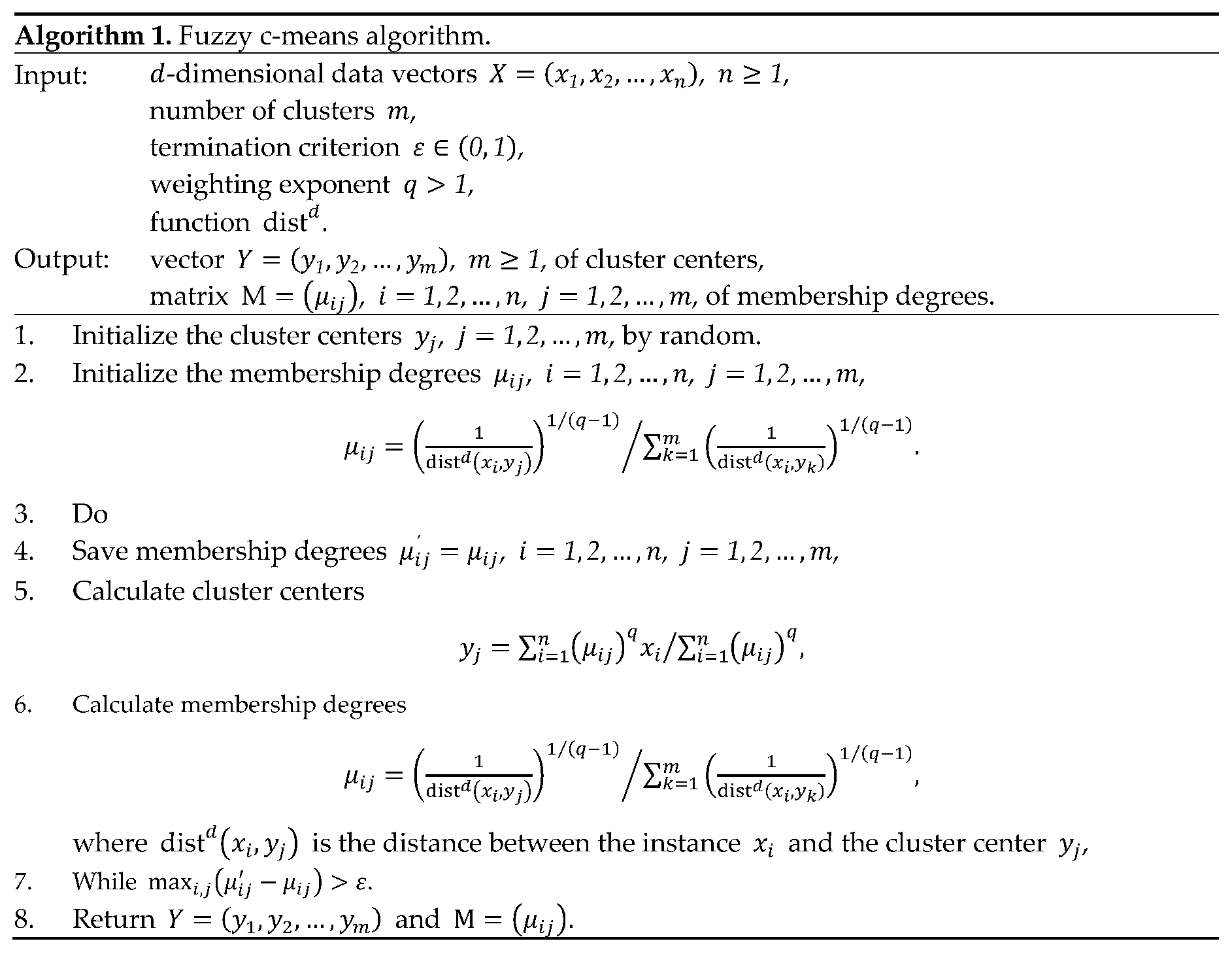
In the original version [13], the fuzzy c-means algorithm uses the Euclidean distance
and in the succeeding versions [16,17] the other distance measures were applied.
In this paper, we suggest to use the logical distance measure based on the uninorm and absorbing norm which results in more accurate recognition of the cluster centers.
2.2. Uninorm and Absorbing Norm
Uninorm [22] and absorbing norm [23] are the operators of fuzzy logic which extend Boolean operators and are used for aggregating truth values.
Uninorm aggregator with neutral element is a function satisfying the following properties [22]; :
- a.
- Commutativity: ,
- b.
- Associativity: ,
- c.
- Monotonicity: implies ,
- d.
- Identity: for some ,
and such that if , then is a conjunction operator and if , then is a disjunction operator.
An absorbing norm aggregator with absorbing element is a function satisfying the following properties [23]; :
- a.
- Commutativity: ,
- b.
- Associativity: ,
- c.
- Absorbing element: for any .
Operator is a fuzzy analog of the negated operator.
Let and be invertible, continuous, strictly monotonously increasing functions with the parameters such that
- a.
- , ,
- b.
- , ,
- c.
- , .
Then, for any hold [24]
and for the bounds and the values of the operators and are defined in correspondence to the results of Boolean operators.
If and , then the interval with the operators and form an algebra [20,25]
in which uninorm acts as a summation operator and absorbing norm acts as a multiplication operator. In this algebra, neutral element is zero value for summation and absorbing element is a unit value for multiplication. Note that in contrast to the algebra of real numbers, in the algebra holds despite different meanings of these values.
The inverse operators in this algebra are
In addition, negation operator is defined as
In the paper [20] it was demonstrated that the functions and satisfy the requirements of quantile functions of probability distributions. Along with that any function satisfying the indicated above requirements and its inverse are also applicable.
Here we will assume that the functions are equivalent. In the simulations, we will use the functions
where , .
3. Results
We start with the definition of logical distance based on the uninorm and absorbing norm and then present the suggested algorithm. In the last subsection we consider numerical simulations and compare the suggested algorithm with the known method.
3.1. Logical Distance Based on the Uninorm and Absorbing Norm
Let be two truth values. Given neutral element and absorbing element , fuzzy logical dissimilarity of the values and is defined as follows:
where the value
is a fuzzy logical similarity of the values and .
If , we will write instead of and instead of .
Lemma 1.
If , then the function is a semi-metric in the algebra .
Proof.
To prove the lemma, we need to check the following three properties:
- a.
- .
By commutativity and identity properties of the uninorm holds:
Then, by the property of absorbing element holds
and
- b.
- if .
If , then either
or
Thus,
and
- c.
- .
It follows directly from the commutativity of the absorbing norm.
Lemma is proven. □
Using the dissimilarity function, we define the fuzzy logical distance between the values as follows ():
Lemma 2.
If , then the function is a semi-metric in the algebra of real numbers on the interval .
Proof.
Since for any and any both , and , and by the properties a and b of semi-metric, holds
- a.
- If , then and
- b.
- If , then . So and
- c.
- Symmetryfollows directly from the symmetry of the dissimilarity . □
An example of the fuzzy logic distance between the values with is shown in Figure 1.a. For comparison, Figure 1.b shows the Euclidean distance between the values .
It is seen that the fuzzy logical distance better separates the close values and less sensitive to the far values than the Euclidean distance.
Now let us extend the introduced fuzzy logical distance to multidimensional variables.
Let
be -dimensional vectors such that each vector , , is a point in a -dimensional space.
The fuzzy logical dissimilarity of the points and , , is defined as follows:
where, as above, the value
is a fuzzy logical similarity of the points and .
Let . Then, as above, the fuzzy logical distance between the points and , , is
Lemma 3.
If , then the function is a semi-metric in the algebra , .
Proof.
This statement is a direct consequence of lemma 1 and the properties of the uninorm.
- a.
- .
If then for each
Then,
and finally
- b.
- if .
If , then for each
Then,
and
- c.
- .
It follows directly from the symmetry of the dissimilarity for each and commutativity of the uninorm. □
Lemma 4.
If , then the function is a semi-metric on the hypercube , .
Proof.
The proof is literally the same as the proof of lemma2. □
The suggested algorithm uses the introduced function as a distance measure between the instances of the data.
3.2. The c-Means Algorithm with Fuzzy Logical Distance
The suggested algorithm considers the instances of the data as truth values and uses Algorithm 1 with the fuzzy logical distance on these values.
As above, assume that the raw data is represented by the -dimensional vectors
where , , , , is a data instance.
Since function requires the values from the hypercube , , vector must be normalized
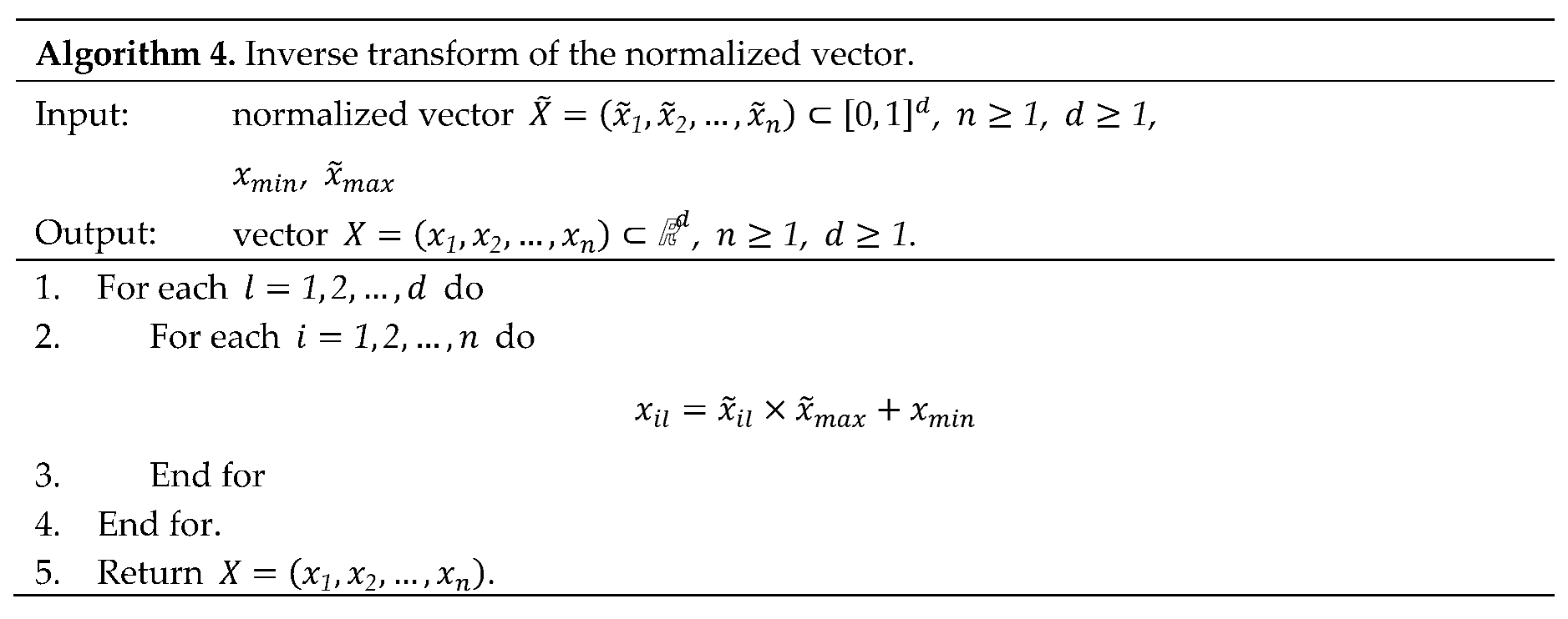
and the algorithm should be applied to the normalized data vector . After definition of the cluster centers , the inverse normalization must be applied to the vector
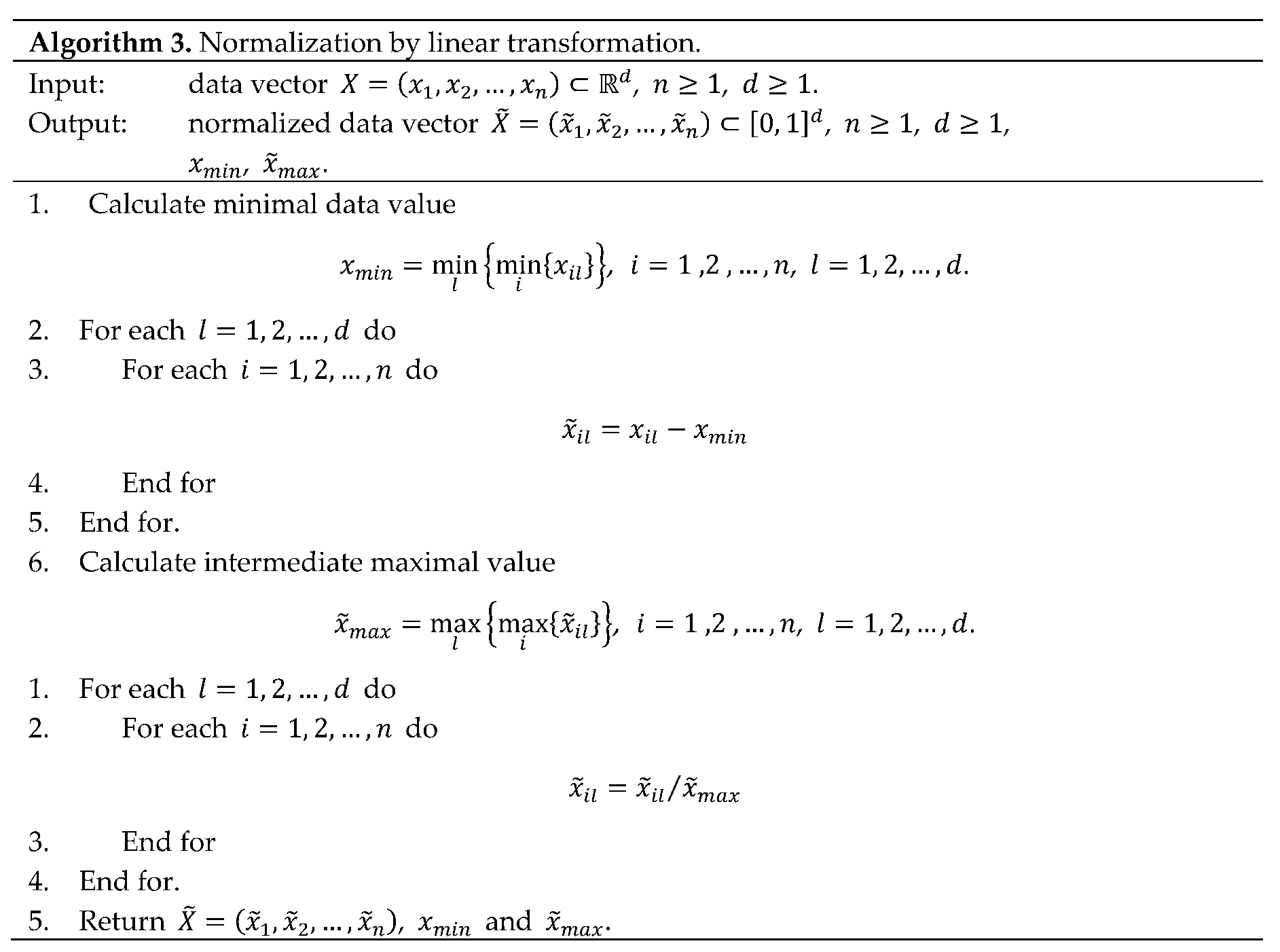
Normalization can be conducted by several methods; in Appendix A we present a simple Algorithm 3 of normalization by linear transformation. The inverse transformation is provided by the Algorithm 4 also presented in Appendix A.
In general, the suggested Algorithm 2 follows the Bezdek fuzzy c-means algorithm 1, however differs in the distance function and in the initialization of the cluster centers , , and, consequently, – in the definition of the number of clusters.
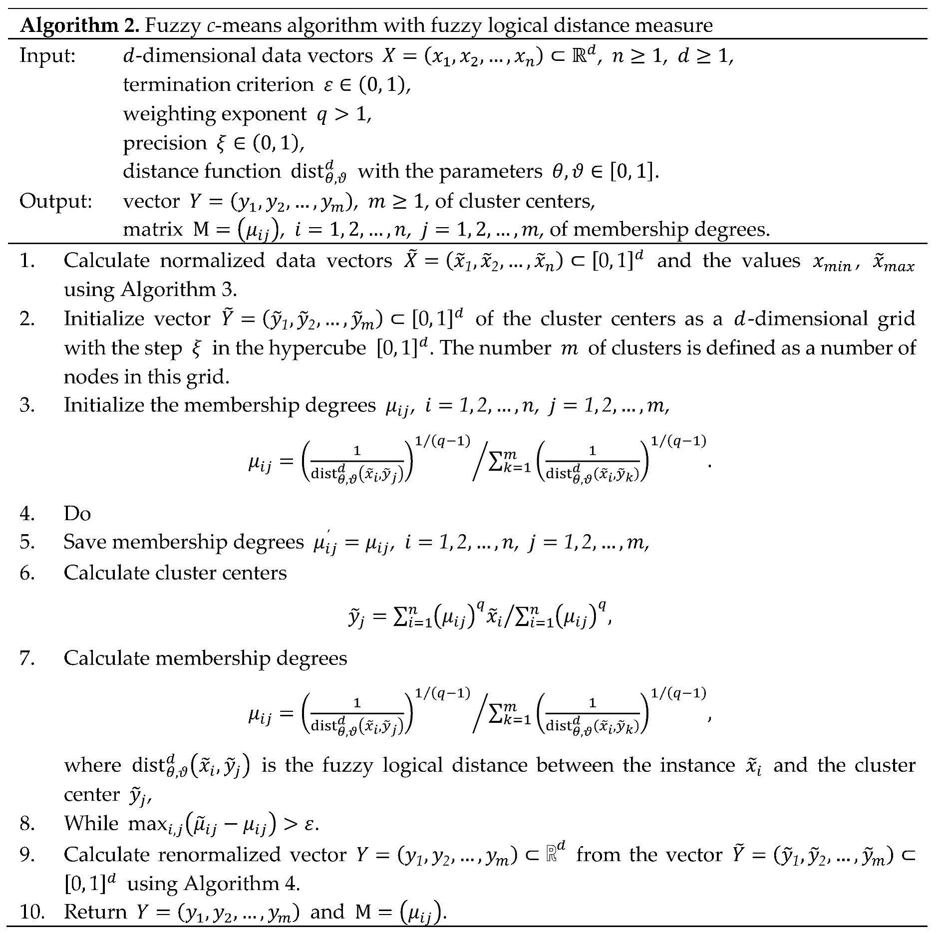
The main difference between the suggested Algorithm 2 and the original Bezdek fuzzy c-means Algorithm 1 [13,14] and the known Gustafson-Kessel [16] and Gath-Geva [17] is the use of the fuzzy logical distance . The use of this distance requires normalization and renormalization of the data.
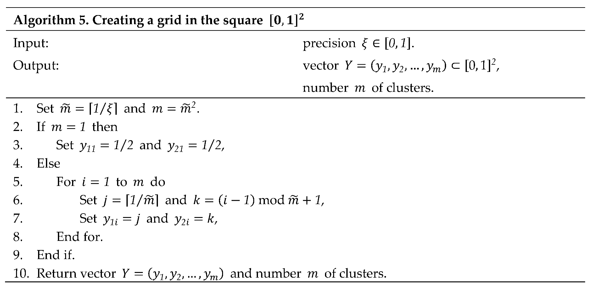
The other difference is in the need of the initialization of the cluster centers as a grid in the algorithm’s domain. Such initialization is required because of quick convergence of the algorithm; thus, the even distribution of the initial cluster centers avoids missing the clusters. A simple algorithm 5 for creating a grid in the square is outlined in Appendix A.
Let us consider two main properties of the suggested algorithm.
Theorem 1.
Algorithm 2 converges.
Proof.
Convergence of the algorithm 2 follows directly from the fact that is a semi-metric (see lemma 4).
In fact, in the lines 3 and 7 of the algorithm holds
and the algorithm converges. □
Theorem 2.
Time complexity of the Algorithm 2 is , where is the dimensionality of the data, is the number of clusters, is the number of instances in the data and is the number of iterations.
Proof.
At first, consider calculation of the fuzzy logical distances , , . Complexity of this operation is for each dimension ; thus, calculation of the distances has a complexity .
Now let us consider the lines of the algorithm. Normalization of the data vector (line 1) requires steps and initialization of the cluster centers (line 2) requires steps (see Algorithm 3 in Appendix A).
Initialization of the membership degrees (line 3) requires steps for each dimension that gives .
In the do-while loop, saving the membership degrees (line 5) requires , calculation of the cluster centers given the membership degrees (line 6) requires steps and calculation of the membership degrees (line 7) requires, as above, steps for each dimension that gives .
Finally, renormalization of the vector of the cluster centers (line 9) requires steps.
Thus, initial (lines 1-3) and final (9) operations of the algorithm require
steps and each iteration requires
Then, for iterations it is required
steps. □
Note that in the considerations above we assumed that which supported the semi-metric properties of the function . Along with that, in practice these parameters can differ and, despite the absence of formal proofs, the use of the function with can provide essentially better clustering.
3.3. Numerical Simulations
In the first series of simulations, we will demonstrate that the suggested Algorithm 2 with fuzzy logical distance results in more precise centers of the clusters than the original Algorithm 1 with Euclidean distance.
For this purpose, in the simulations we generate a single cluster as normally distributed instances with the known center and apply Algorithms 1 and 2 to these data. As a measure of the quality of the algorithms we use the mean squared error (MSE) in finding the center of the cluster center and the means of standard deviations of the calculated clusters centers.
To avoid the influence of the instance values, in the simulations we considered the normalized data. An example of the data (white circles) and the results of the algorithms (gray diamonds for Algorithm 1 and black pentagrams for Algorithm 2) are shown in Figure 2.
The simulations were conducted with different numbers of clusters by the series of trials. The results were tested and compared by the one-sample and two-sample Student’s -tests.
In the simulations we assumed that the algorithm which for a single cluster provides less deviated cluster centers is more precise in the calculation of the cluster centers. In other words, the algorithm which results in the clusters centers concentrated near the actual cluster center is better than the algorithm which results in more dispersed cluster centers.
Results of simulations are summarized in Table 1. In the table, we present the results of clustering of two-dimensional data distributed around the mean .
It is seen that both algorithms result in cluster centers close to the actual cluster center and the errors in calculating the centers are extremely small. Additional statistical testing by Student’s -test demonstrated that the differences between the obtained clusters centers are not significant with .
Along with that, the suggested Algorithm 2 results in smaller standard deviation than the Algorithm 1 and this difference is significant with . Hence, the suggested Algorithm 2 results in more precise cluster centers than Algorithm 1.
To illustrate these results, let us consider simulations of the algorithms on the data with several predefined clusters.
Consider application of Algorithms 1 and 2 to the data with two predefined clusters with the centers in the points and . The resulting cluster centers with and clusters are shown in Figure 3. Notation in the figure is the same as in Figure 2.
It is seen that clusters centers obtained by Algorithm 2 (black pentagrams) are concentrated closer to the actual cluster centers than the cluster centers obtained by Algorithm 1 (gray diamonds). Moreover, some of the cluster centers obtained by Algorithm 2 are located in the same points while all cluster centers obtained by Algorithm 1 are located in different points.
More clearly the observed effect is seen on the data with several clusters. Figure 4 shows the results of Algorithms 1 and 2 applied to the data with predefined clusters.
It is seen that the cluster centers calculated by Algorithm 2 are concentrated at the real centers of the clusters and, as above, several centers are located at the same points. Hence, the suggested Algorithm 2 allows more correct definition of the cluster centers and consequently, more correct clustering.
To illustrate the usefulness of the suggested algorithm in recognition of the number of clusters and analysis of the data structure, let us compare the results of the algorithm with the results obtained by the MATLAB® fcm function [15] with three possible distance measures: Euclidean distance, Mahalanobis distance [16] and exponential distance [17]. These algorithms were applied to data instances distributed around centers; the obtained results are shown in Figure 5.
It is seen that the suggested algorithm (Figure 5.a) correctly recognizes the real centers of the clusters and locates the cluster centers close to these real centers. In contrast, the known algorithms implemented in MATLAB® do not recognize real centers of the clusters and, consequently, do not define correct number of the clusters and locations of their centers. The function fcm with Euclidean and Mahalanobis distance measures (Figure 5.b,c) results in two cluster centers and the function fcm with exponential distance (Figure 5.d) results in three cluster centers. Note that the use of Euclidean and Mahalanobis distance measures leads to very similar results.
Thus, recognition of the real cluster centers which are the centers of distributions of the data instances can be conducted in two stages. At first, the cluster centers are defined by application of the suggested algorithm to the raw data, and at second, the cluster centers by application of k-means to the cluster centers found at the first stage. The resulting cluster centers indicate the real cluster centers.
4. Discussion
The suggested algorithm of fuzzy clustering follows the line of c-means fuzzy clustering algorithms and differs from the known methods in the used distance measure.
The suggested fuzzy logical distance is a semi-metric based on the introduced semi-metric in the algebra of truth values with uninorm and absorbing norm. The meaning of these semi-metrics is the following.
Assume that some statements and are considered by a group of observers and each of the observers expresses an opinion about the truthiness of these statements. Assuming that the observers are independent, the statements and can be considered as point in the -dimensional space and then the suggested semi-metric is a distance between these statements.
In other words, the fuzzy logical distance measures allow comparing the statements based on their subjective truthiness.
In the paper, we considered the fuzzy logical distance based on the uninorm and absorbing norm which, in their turn, use the sigmoid generating functions. As a result, the fuzzy logical distance effectively separates the data instances which leads to more precise calculation of the cluster centers and more quick convergence of the algorithm.
An additional advantage of the algorithm is the possibility of tuning its activity by two parameters: neutral element and absorbing element . As indicated above, better results of the clustering can be obtained using non-equal values and . An inequality of these parameters slightly disturbs the semi-metric properties of the distance measures, however, leads to better separation of close but different points.
The weakness of the algorithm is the need of normalization of the data and then renormalization of the obtained clusters centers. However, since both operations are conducted in polynomial time, this disadvantage is not a serious drawback.
The suggested algorithm of fuzzy clustering can be used for solving the clustering problems instead of or together with the known algorithms, for recognition of the centers of distributions of the data instances and can form a basis for development of the methods of comparison of multivariate samples.
Author Contributions
Conceptualization, E.K. and A.N.; methodology, A.R.; software, E.K. and A.N.; validation, E.K., A.N. and A.R.; formal analysis, E.K. and A.R.; investigation, E.K. and A.N.; resources, E.K. and A.N.; data curation, A.N.; writing—original draft preparation, E.K.; writing—review and editing, A.N. and A.R.; supervision, A.R. All authors have read and agreed to the published version of the manuscript.
Funding
This research received no external funding.
Data Availability Statement
No new data were created or analyzed in this study. Data sharing is not applicable to this article.
Conflicts of Interest
The authors declare no conflicts of interest.
Appendix A
Appendix includes three supplementary algorithms which are used in the suggested Algorithm 2.
References
- Raiffa, H. Decision Analysis. Introductory Lectures on Choices under Uncertainty. Addison-Wesley: Reading, MA, USA, 1968.
- Triantaphyllou, E. Multi-Criteria Decision Making Methods: A Comparative Study. Springer Science + Business Media: Dordrecht, Netherlands, 2000.
- López, L. M.; Ishizaka, A.; Qin, J.; Carrillo, P. A. A. Multi-Criteria Decision-Making Sorting. Methods Applications to Real-World Problems. Academic Press / Elsevier: London, UK, 2023.
- Han, J.; Kamber, M.; Pei, J. Data Mining: Concepts and Techniques. Morgan Kaufmann / Elsevier: Waltham, MA, USA, 2012.
- Ghanaiem, A; Kagan, E.; Kumar, P.; Raviv, T.; Glynn, P.; Ben-Gal, I. Unsupervised classification under uncertainty: the distance-based algorithm. Mathematics 2023, 11 (23), 4784. [CrossRef]
- Ratner, N.; Kagan, E.; Kumar, P.; Ben-Gal, I. Unsupervised classification for uncertain varying responses: the Wisdom-In-the-Crowd (WICRO) algorithm. Knowledge-Based Systems 2023, 272, 110551. [CrossRef]
- Everitt, B. S.; Landau, S.; Leese, M.; Stahl, D. Cluster analysis. Jonh Wiley & Sons: Chichester, UK, 2011.
- Aggarwal, C. C. An introduction to cluster analysis. In Data Clustering: Algorithms and Applications; Aggarwal, C. C., Reddy C. K., Eds.; Chapman & Hall / CRC / Taylor & Francis, 2014.
- Lloyd, S. P. Least squares quantization in PCM. IEEE Trans. Information Theory, 1982, 28(2), 129-137. [CrossRef]
- Forgy, E. W. Cluster analysis of multivariate data: efficiency vs. interpretability of classifications; Abstract. Biometrics, 1965, 21(3), 768-769.
- Hartigan, J. A.; Wong, M. A. A k-means clustering algorithm. J. Royal Statistical Society, Series C, 1979, 28(1), 100-108.
- MATLAB® Help Center. k-Means Clustering. Available online: https://www.mathworks.com/help/stats/k-means-clustering.html (accessed on 12.04.2025).
- Bezdek, J. C. Fuzzy Mathematics in Pattern Classification. Ph.D. Thesis, Cornell University, Ithaca, NY, USA, 1973.
- Bezdek, J. C. Pattern Recognition with Fuzzy Objective Function Algorithms. Springer: New York, NY, USA, 1981.
- MATLAB® Help Center. Fuzzy Clustering. Available online: https://www.mathworks.com/help/fuzzy/fuzzy-clustering.html (accessed on 12.04.2025).
- Gustafson, D.; Kessel, W. Fuzzy clustering with a fuzzy covariance matrix. In Proceedings of IEEE Conference on Decision and Control, San Diego, CA, USA, 10-12 Jan 1979.
- Gath, I.; Geva, A. B. Unsupervised optimal fuzzy clustering. IEEE Trans. Pattern Analysis and Machine Intelligence 1989, 11 (7), 773-780.
- Li, J.; Lewis, H. W. Fuzzy clustering algorithms – review of the applications. In Proceedings of IEEE International Conference on Smart Cloud, New York, NY, USA, 18-20 Nov 2016.
- Höppner, F.; Klawonn, F.; Kruse, R.; Runkler, T. Fuzzy Cluster Analysis: Methods for Classification, Data Analysis and Image Recognition. Jonh Wiley & Sons: Chichester, UK, 2019.
- Kagan, E.; Rybalov, A.; Siegelmann, H.; Yager, R. Probability-generated aggregators. Int. J. Intelligent Systems 2013, 28 (7), 709-727.
- Kagan, E.; Rybalov, A.; Yager, R. Multi-valued Logic for Decision-Making under Uncertainty; Springer-Nature / Birkhäuser: Cham, Switzerland, 2025.
- Yager, R. R.; Rybalov, A. Uninorm aggregation operators. Fuzzy Sets and Systems 1996, 80, 111-120. [CrossRef]
- Rudas, I. J. New approach to information aggregation. Zbornik Radova 2000, 2, 163–176.
- Fodor, J.; Yager, R.; Rybalov, A. Structure of uninorms. Int. J. Uncertainty, Fuzziness and Knowledge-Based Systems 1997, 411-427.
- Fodor, J.; Rudas, I. J.; Bede, B. Uninorms and absorbing norms with applications to image processing. In Proceedings of the 4th Serbian-Hungarian Joint Symposium on Intelligent Systems, Subotica, Serbia, 29-30 Sept 2006.
Figure 1.
(a) Fuzzy logic distance between the values with ; (b) Euclidean distance between the values .
Figure 1.
(a) Fuzzy logic distance between the values with ; (b) Euclidean distance between the values .
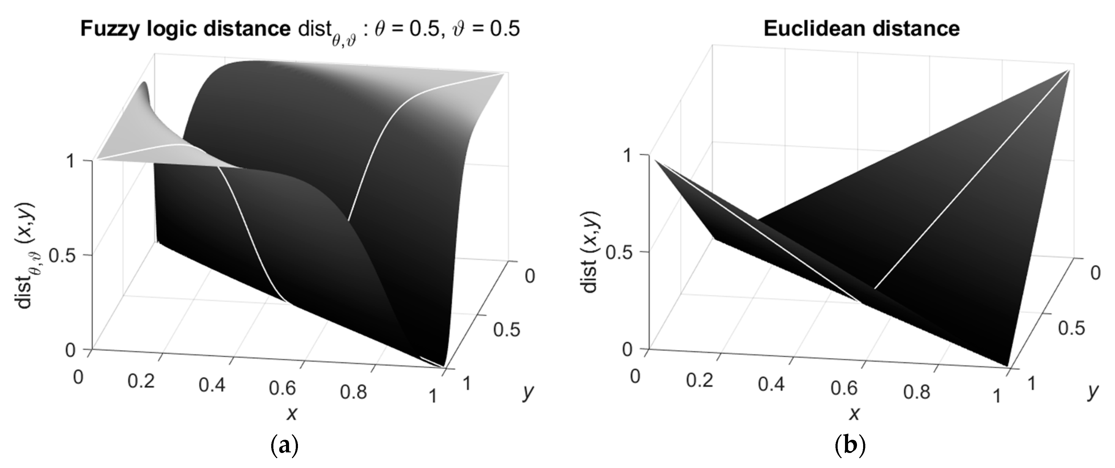
Figure 2.
Example of the data and the resulting cluster centers for a single cluster of normally distributed instances. Number of instances is , number of clusters is , and number of iterations . Initially, the cluster centers are in the nodes of the grid and are depicted by black points. The instances are distributed normally around the mean and are shown by white circles. The cluster centers calculated by the Algorithm 1 with Euclidean distance are depicted by gray diamonds and the cluster centers calculated by the Algorithm 2 with fuzzy logical distance are depicted by black pentagrams.
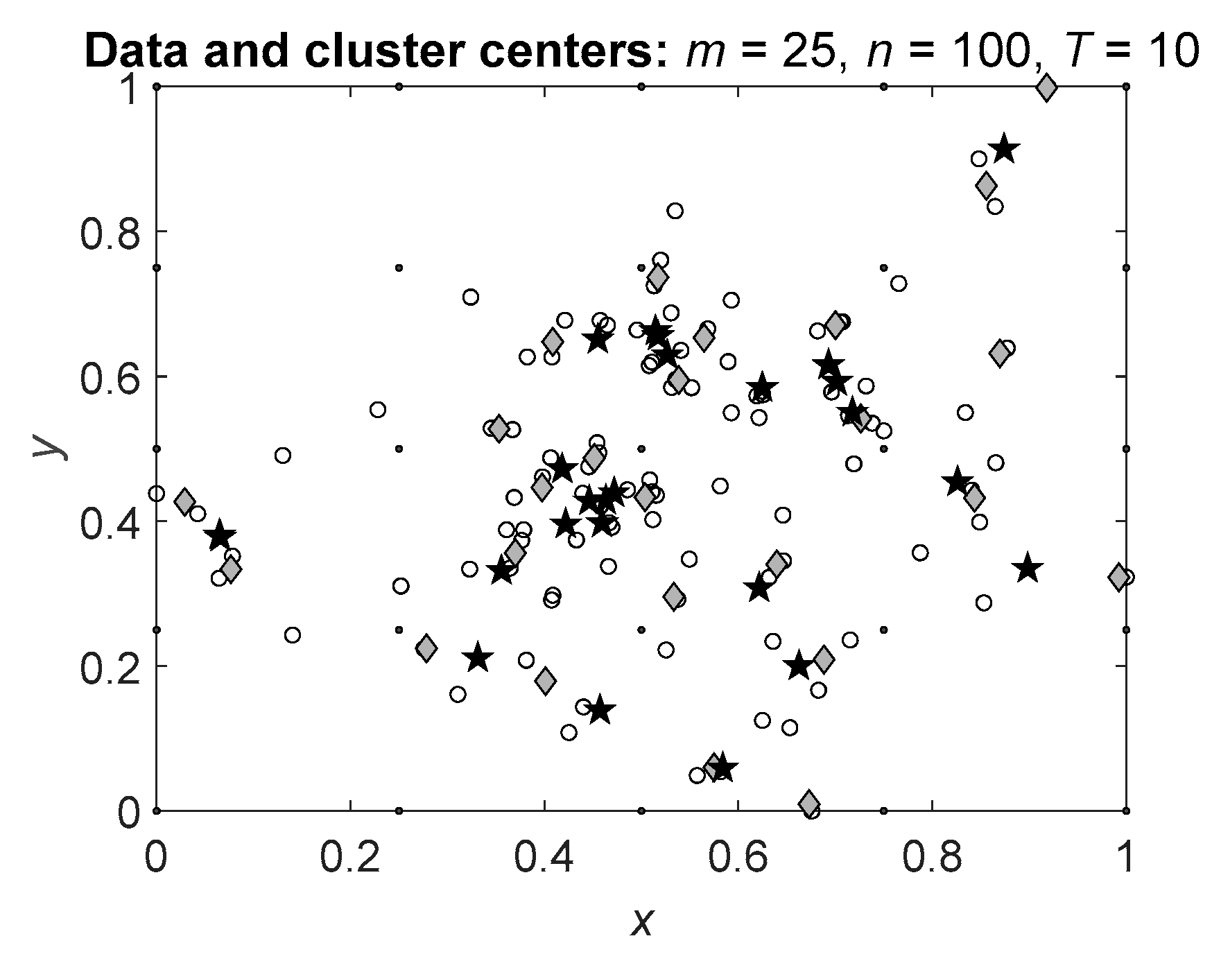
Figure 3.
Data with two predefined clusters and cluster centers calculated by the Algorithms 1 and 2: (a) number of clusters ; (b) number of clusters .
Figure 3.
Data with two predefined clusters and cluster centers calculated by the Algorithms 1 and 2: (a) number of clusters ; (b) number of clusters .
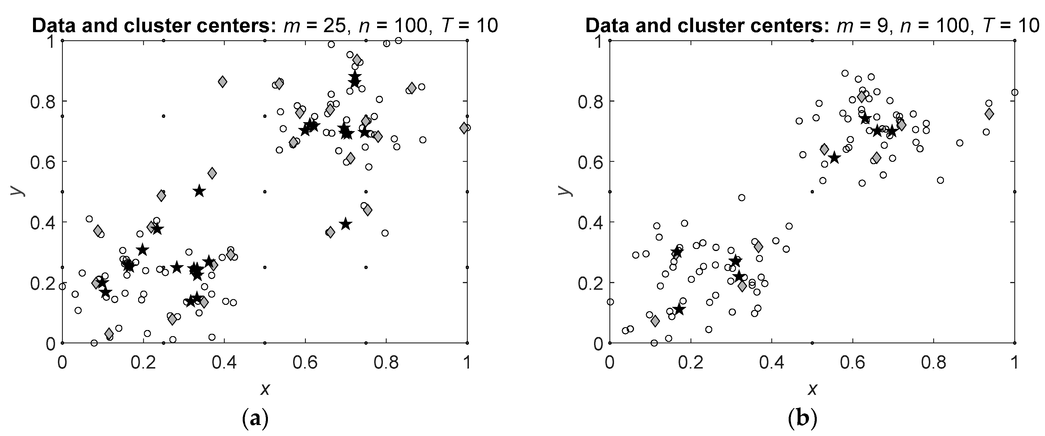
Figure 4.
Data with ten predefined clusters and cluster centers calculated by the Algorithms 1 and 2: (a) number of clusters ; (b) number of clusters .
Figure 4.
Data with ten predefined clusters and cluster centers calculated by the Algorithms 1 and 2: (a) number of clusters ; (b) number of clusters .
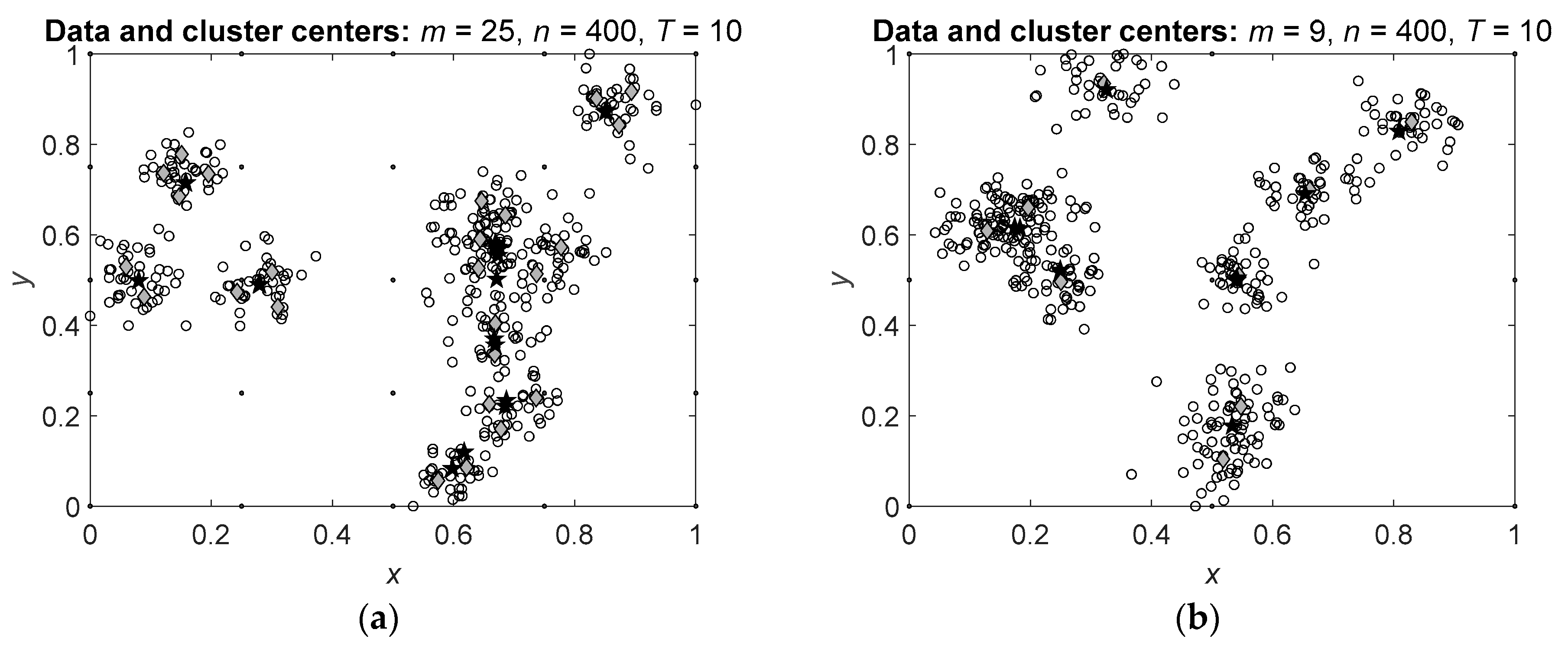
Figure 5.
Cluster centers calculated by the suggested Algorithm 2 (a) and by the MATLAB® fcm function with Euclidean (b), Mahalanobis (c) and exponential (d) distance measures. In all cases, the real number of clusters is and the number of data instances is . Algorithm 2 starts with clusters and is terminated after iterations, and function fcm defines an optimal number of clusters by trials with the number of clusters from to .
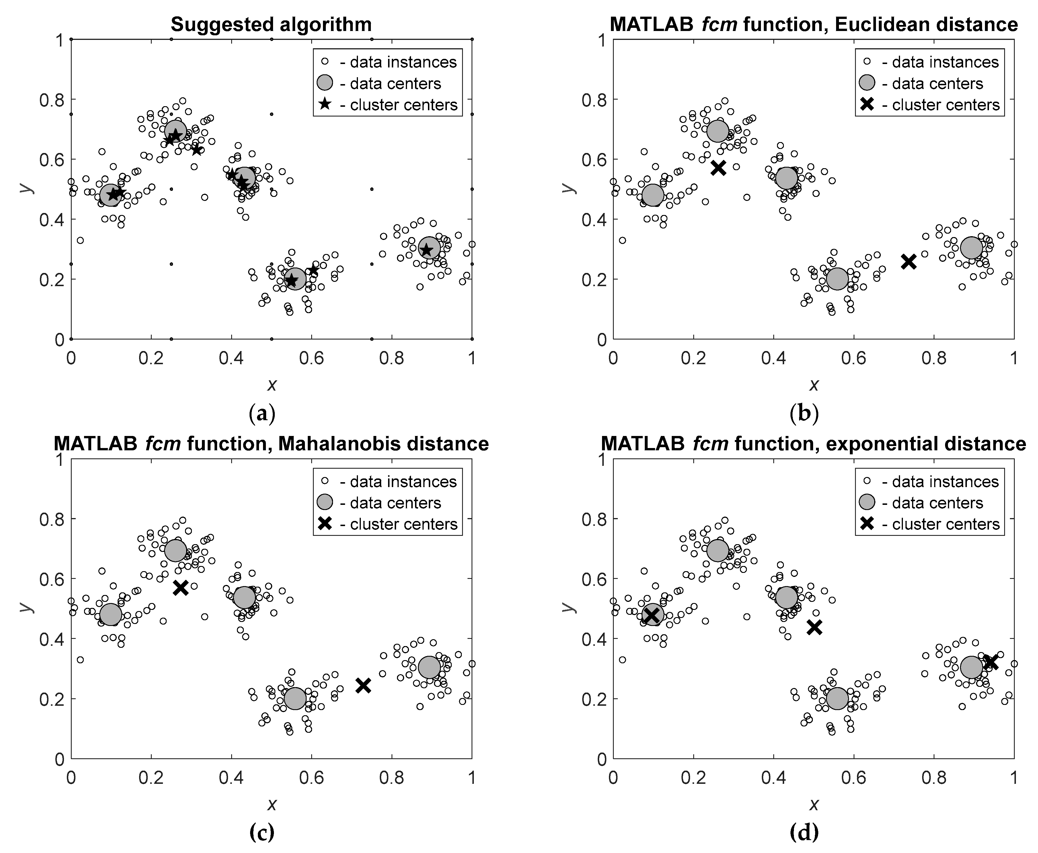

Table 1.
Results of simulations for each dimension: means , of the instances which are the centers of the cluster, mean squared errors , of the centers calculated by the Algorithms 1 and 2, means of the standard deviations , of the cluster centers calculated by the Algorithms 1 and 2 and significance of the difference between standard deviations of the cluster centers calculated by the Algorithms 1 and 2.
| #instances, #clusters | Source |
Mean |
MSE |
Mean STD |
Significance of the STD’s difference |
|
, |
Data |
|
− | − | − |
| Algorithm 1 |
|
|
|
||
| Algorithm 2 |
|
|
|
||
|
, |
Data |
|
− | − | − |
| Algorithm 1 |
|
|
|||
| Algorithm 2 |
|
|
|||
|
, |
Data |
|
− | − | |
| Algorithm 1 |
|
|
|||
| Algorithm 2 |
|
|
Disclaimer/Publisher’s Note: The statements, opinions and data contained in all publications are solely those of the individual author(s) and contributor(s) and not of MDPI and/or the editor(s). MDPI and/or the editor(s) disclaim responsibility for any injury to people or property resulting from any ideas, methods, instructions or products referred to in the content. |
© 2025 by the authors. Licensee MDPI, Basel, Switzerland. This article is an open access article distributed under the terms and conditions of the Creative Commons Attribution (CC BY) license (http://creativecommons.org/licenses/by/4.0/).
Copyright: This open access article is published under a Creative Commons CC BY 4.0 license, which permit the free download, distribution, and reuse, provided that the author and preprint are cited in any reuse.


