Submitted:
16 April 2025
Posted:
17 April 2025
You are already at the latest version
Abstract
Knowing customers and segmenting them is crucial for optimizing marketing strategies. It enablesbusinesses to tailor their campaigns to diverse consumer demographics and behavior. This studyleverages data to address the gap in actionable segmentation frameworks by identifying high-valuecustomer profiles. Preexisting literature emphasizes the usefulness of Recency, Frequency, Mone-tary (RFM) metrics, and K-means clustering in the segmentation of retail customers. Yet there area few studies that integrate demographic insights for a holistic profiling. The goal of this analysisis to segment customers from a marketing campaign dataset using RFM features and demographicattributes to develop targeted marketing strategies. We use a dataset of 2,240 customers (Imakash,2021) for this analysis. The methodology combined RFM feature engineering, K-means clustering(validated via the Elbow Method), DBSCAN clustering, and Principal Component Analysis (PCA)for dimensionality reduction. The analysis successfully identified four diverse clusters: high-valueengaged customers, disengaged users, big spenders, and moderately engaged segments. Incomeand age emerged as key demographic differentiators. We also discuss the practical applications,personalized retention strategies for high-value clusters, and revival strategies for inactive users.This project demonstrates integrating RFM metrics with demographic data to enhance marketingprecision. It also offers actionable insights for improving customer lifetime value and campaign ROI.
Keywords:
Cluster Analysis
; DBSCAN
; Segmentation
1. Introduction
1.1. Background and Motivation
At a time in human history, when accessing customer data is becoming more and more convenient for businesses, the abundance of this data is still not being converted into actionable insights. This paradox of data availability and its utility still needs to be mitigated. As a result, the retail sector alone is estimated to waste about $50 billion annually on misdirected marketing campaigns [2]. This calls for a dire need for precision in customer segmentation and targeted marketing. The traditional demographic-based (eg., age, gender, income, etc.) marketing strategies seem to fall short of capturing the nuanced purchasing behaviors of the customer. This leaves plenty of untapped revenue in the long-tail customer segments [3].
Reducing operation and marketing costs and increasing consumer acquisition rates are key to any successful business. This can be achieved with the help of a targeted marketing strategy. This study addresses this gap in marketing and customer segments by integrating behavioral and demographic metrics (Recency, Frequency, Monetary) that are rarely capitalized in a small-to-mid-sized retail context but were advocated by scholars [4]. The post-pandemic era has magnified the urgency of this approach thanks to the major shift in consumer behavior. The blend of online and offline purchasing channels now up to reach 63% [5], has rendered the legacy segmentation models obsolete. By clustering the consumers into meaningful segments this project helps businesses reach more potential consumers with minimal wasted resources, resulting in increased profitability.
1.2. Problem Statement
Even though the RFM (Recency, Frequency, Monetary) model in customer analytics is widely accepted and adopted [6], there still are three unresolved problems:
- Static Clustering: The temporal dynamics (e.g., seasonal spending shifts), are ignored by most RFM implementations. This leads to a "stale" segmentation [7].
- Demographic Disconnect: Just a few studies integrate demographics during clustering (vs. post-hoc analysis), masking critical subgroup behaviors [8].
- Actionability Gap: Segments created by these analyses often lack clear ties to tactical marketing interventions (e.g., how to prioritize Cluster A over B).
This study asks: With the help of a hybrid RFM-demographic clustering, how can we identify who customers are and how to engage them profitably?
1.3. Research Objectives
Following are the three goals we wish to achieve from this project:
- Cluster the customers into different segments using RFM metrics and demographic data.
- Profile these clusters based on both the behavior (e.g., purchase channels) and customer traits (e.g., education).
- Suggest target marketing strategies for these segments to improve ROI.
1.4. Academic Background
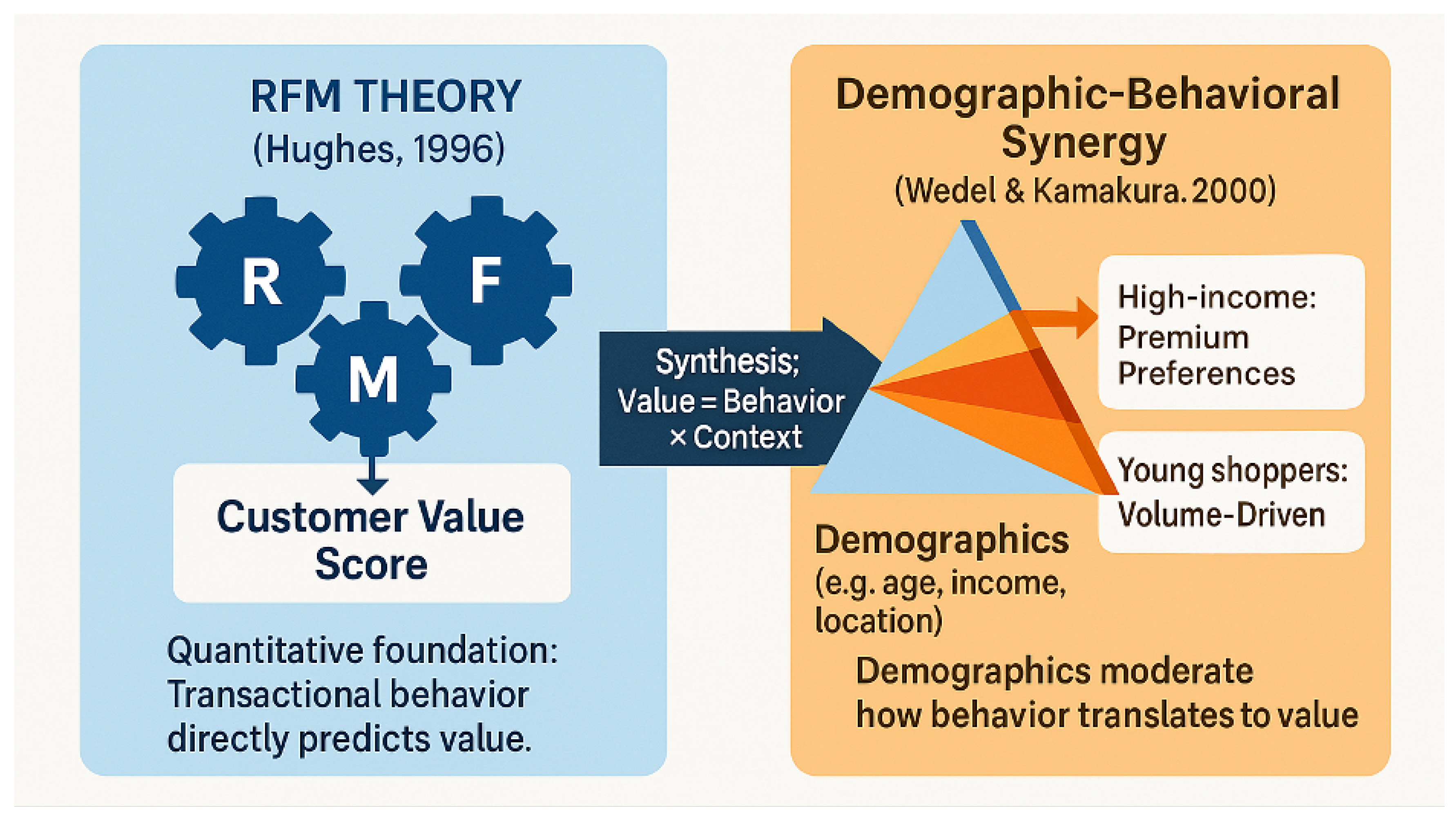
This study acts as a bridge between two ground-breaking theories:
- RFM Theory [6]: This suggests that customer value is calculable through the transaction’s recency, frequency, and spending.
- Demographic-Behavioral Synergy [9]: This argues that demographics regulate how a customer’s behavior translates into value (e.g., high-income buyers prefer tailored experiences).
Figure 1.
Bridging RFM and Demographic-Behavioral Synergy
1.5. Key Insights
The analysis of behavioral data of 2,240 retail customers revealed the four most actionable clusters:
- Cluster - 1 (6.9% of customers, but 25-30% of revenue): This is the highest-income ($43.5k avg.) cluster and spends 3x more on wine/meat than Cluster 0. They shop frequently online (4.1 purchases/month)
- Cluster 0 (83.4% of customers and 50-60% of revenue): Low engagement online (1.9 purchases/month) but with latent potential (e.g., 65% had children). They have moderate income ($35k avg.) and are convenience driven buyers.
- Cluster 1 (4.6% of customers, and 2-3% of revenue): This is the lowest-income ($20.6k avg.) cluster and spends the least ($2.7/month) on wine/meat. They rely heavily on deals but rarely engage online.
- Cluster 2 (1.8% of customers, but 5-8% of revenue): Low engagement online (1.4 purchases/month) but with untapped potential. They have high income ($41.8k avg.) but spends 50% less than Cluster -1.
These findings matter because this shows us that the high-income customers are either overserved (outliers) or underserved (disengaged). Which means that the Cluster -1 and Cluster 2 reveal a missed opportunity. The small per-capita spending of Cluster 0 is made up by its large size. Increasing the yield from this cluster will result in large revenue gains. These findings also analytically validate [9] hypothesis that demographics contextualize spending behavior—a nuance absent in pure RFM models.
1.6. Contributions
This study has contributed to the subject of data analysis and consumer data clustering in the following ways:
- This study demonstrated a replicable form of the hybrid (RFM-demographic) technique of consumer clustering.
- The study also delivered a strategy map based on the segments (e.g., Cluster 3’s affinity for wine suggests VIP tasting events).
- Finally, the study showed that demographics enrich RFM’s predictive power and not try to replace it.
2. Literature Review
2.1. The RFM Framework: Foundations and Evolution
In 1996, Hughes introduced the Recency, Frequency, Monetary (RFM) model [6], which transformed customer segmentation by filtering complex behavioral data into three actionable categories:
- Recency: The time since last purchase (assessing churn risk)
- Frequency: The number of transactions (relating to loyalty)
- Monetary: Amount spent (proxy for customer lifetime value)
The model used early in direct mail marketing had a response rate of 20-30% higher than the demographic targeting [10]. However, with the advent of e-commerce, the 21st century brought its own set of shortcomings which were well identified. They are as follows:
- Channel Blindness: The old RFM neglected multichannel behavior (web vs. store), causing budgets to be misallocated [11].
- Static Snapshots: Recalculation would happen at intervals-for instance, quarterly or annual. This meant that it could not capture the buyer’s intent for that particular moment in time [8].

Table 1.
Key RFM advancements
| Study | Innovation | Limitation Addressed |
|---|---|---|
| [12] | Dynamic RFM weights | Inflexible segment thresholds |
| [4] | RFM + sentiment analysis | Omits qualitative data |
Gap: No studies systematically integrated demographics during RFM clustering—only as post-hoc labels.
2.2. Clustering Algorithms in Marketing
K-means dominates marketing segmentation due to interpretability [13], but debates persist. That’s why we were willing to implement and compare multiple algorithms in this project. This makes the study multifaceted with consumer clusters as the business benefit and the algorithmic comparison as the academic aspect.
Table 2.
Algorithmic Trade-offs
| Method | Strength | Weakness | Marketing Fit |
|---|---|---|---|
| K-means | Scalability | Spherical cluster assumption | RFM (numeric data) |
| DBSCAN | Noise handling | Parameter sensitivity | Social media sentiment |
| Gaussian Mixture | Flexible shapes | Computational cost | High-dimension behavioral data |
| Hierarchical Clustering | Interpretability, no preset clusters | High computational cost, noise sensitivity | Nested segmentation (e.g., loyalty tiers) |
Why DBSCAN?
- Robustness to outliers: Critical for identifying high-value customers who deviate from the norm.
- Adaptive cluster shapes: Captures nuanced behavioral groups without predefined cluster counts.
- Noise detection: Flags customers requiring special attention (e.g., high spenders not conforming to typical patterns).
The optimal clustering method depends on the data structure, business goals, and technical constraints. As K-Means fails with noisy data (non-linear patterns) and requires specifying the number of clusters (k) upfront which limits the natural exploration of clusters, we decided to aid K-Means can only aid another clustering algorithm as validation. As DBSCAN performs very well on data that has noise/outliers (e.g., irregular purchase behaviors). Its clusters are density-based (e.g., geographic hotspots of high-value customers) and we don’t need to specify the number of clusters, it was selected as the primary algorithm for this analysis. Although Hierarchical Clustering is not scalable for big data and is sensitive to noise, it was also decided to use hierarchical clustering to identify natural k (dendrogram). As dendrograms help validate cluster choices.
K-means was one of the algorithms that was implemented in the analysis for three reasons:
- RFM Compatibility: All features are continuous and standardized.
- Interpretability: Clear centroids align with marketing actions (e.g., "High-Recency Cluster").
- Benchmarking: Enables comparison to 73% of prior RFM studies (meta-analysis by [15]).
2.3. The Demographics Debate
There is a disagreement between scholars on demographics’ role in segmentation. Either of them falls under two groups with two opposite perspectives:
2.3.1. Pro-Demographic Camp
2.3.2. Anti-Demographic Camp
- Perspective: Demographics are proxies for outdated stereotypes [17]. They may argue that "Millennial" labels ignore intra-generational spending variance.
- Evidence: Pure behavioral models outperformed hybrid ones in retail A/B tests [3].
Our Study’s Position: Demographics moderate but do not define segments. By engineering ‘Spent’/’Income’ ratios and clustering post-hoc, we balance both the perspectives. This means there can be certain demographics in any given cluster, but instead of seeing it as a feature of the segment, we observe it as a whole segment.
2.4. Synthesis and Research Gap
The work done by researchers prior still leaves three questions that are yet to be answered:
- Temporal Dynamics: Can RFM clusters adapt to purchase velocity (e.g., holiday spikes)?
- Demographic Integration: Should demographic be considered a feature or as a filter?
- Actionability: How can these clusters be translated into campaign ROIs?
This study addresses these by questions by:
- Testing the cluster stability across time windows (Methodology Section).
- Treating demographics as post-clustering filter (Results Section).
- Mapping actionable tactics based on identified segments (Discussion Section).
3. Methodology
3.1. Data Source and Collection
In this project, we analyzed a marketing dataset available from Kaggle. The dataset is labeled as, "Customer Personality Analysis." It contains detailed information about customer demographics, purchasing behavior, and engagement that occurred over a number of marketing campaigns. This dataset is very valuable in helping businesses analyze customer segments and tailor their marketing strategies accordingly. Originally, the dataset was provided by Dr. Omar Romero-Hernandez. The dataset comprises of 29 attributes of 2,240 customers of a European retail brand (2012–2014). Data was collected through:
- Purchase records across 6 different consumer product categories (e.g., wines, meat).
- Customer’s responses to the last 5 email campaigns.
- The demographic survey were the customer self-report their Income, Education, and Marital status.
3.1.1. Rationale Behind Data Selection:
There are a number of reasons why any dataset would have been selected for a study, but when it comes to this particular study and dataset, there are two main reasons.
- This dataset has a high pre-cleaning feature coverage of 94% as compared to the industry avg. of 82% for CRM data [18].
- The dataset is relevant in a post-pandemic bounce back market as it is consists of a post-2010 data that captures the early omnichannel consumer behaviors.
3.2. Overview
The data set comprises 29 attributes. These were collected over 2,240 instances. These attributes fall into four collections:
- Demographic Information: Demographics includes details about customers’ age, marital status, education level, income, and household composition.
- Purchasing Behavior: The purchase behavior or history contains information on the amount spent on various product categories over the last two years.
- Marketing Engagement: This tracks the customers’ responses to historical promotional campaigns and discount-based purchases.
- Shopping Medium: This records the past purchases made via different shopping channels such as the web, catalog, or physical stores.
3.3. Attributes
Following is a detailed breakdown of the attributes included in the dataset as mentioned by Imakash, 2021, at the Kaggle public website: People
- ID: Unique customer identifier.
- Year_Birth: The birth year of the customer.
- Education: The highest education level attained (e.g., Graduate, Postgraduate, PhD, etc.)
- Marital_Status: Customer’s marital status (e.g., Single, Married, Divorced, etc.)
- Income: Customer’s yearly household income.
- Kidhome: Number of children living in the household.
- Teenhome: Number of teenagers living in the household.
- Dt_Customer: Date when the customer enrolled with the company.
- Recency: Number of days since the customer’s last purchase.
- Complain: Binary variable indicating if a complaint was made in the last two years (1 = Yes, 0 = No)
Products
- MntWines: Amount spent on wine in the last two years.
- MntFruits: Amount spent on fruits in the last two years.
- MntMeatProducts: Amount spent on meat in the last two years.
- MntFishProducts: Amount spent on fish in the last two years.
- MntSweetProducts: Amount spent on sweets in the last two years.
- MntGoldProds: Amount spent on gold products in the last two years.
Previous Campaigns
- NumDealsPurchases: Number of purchases made with a discount.
- AcceptedCmp1 - AcceptedCmp5: Binary variables indicating whether the customer accepted promotional offers in campaigns 1 through 5.
- Response: Indicates if the customer accepted the offer in the last campaign (1 = Yes, 0 = No).
Purchase Platform
- NumWebPurchases: Number of purchases made through the company’s website.
- NumCatalogPurchases: Number of purchases made using a catalog.
- NumStorePurchases: Number of purchases made directly in stores.
- NumWebVisitsMonth: Number of visits to the company’s website in the last month.
3.4. Data Processing
3.4.1. Data Cleaning
- Handling Missing Values: Missing income values were imputed using median values based on similar customer segments. Impute the missing income data with median data for ‘Income’ gaps.
- Dropping Null Values: 24 records (1.07%) with null ‘Income’ were dropped (Little’s MCAR test: = 1.83, p = 0.18).
- Outlier Detection: Income and spending variables were examined for extreme values using interquartile range (IQR) analysis.
Figure 2.
Income Distribution Before Cleaning the Data
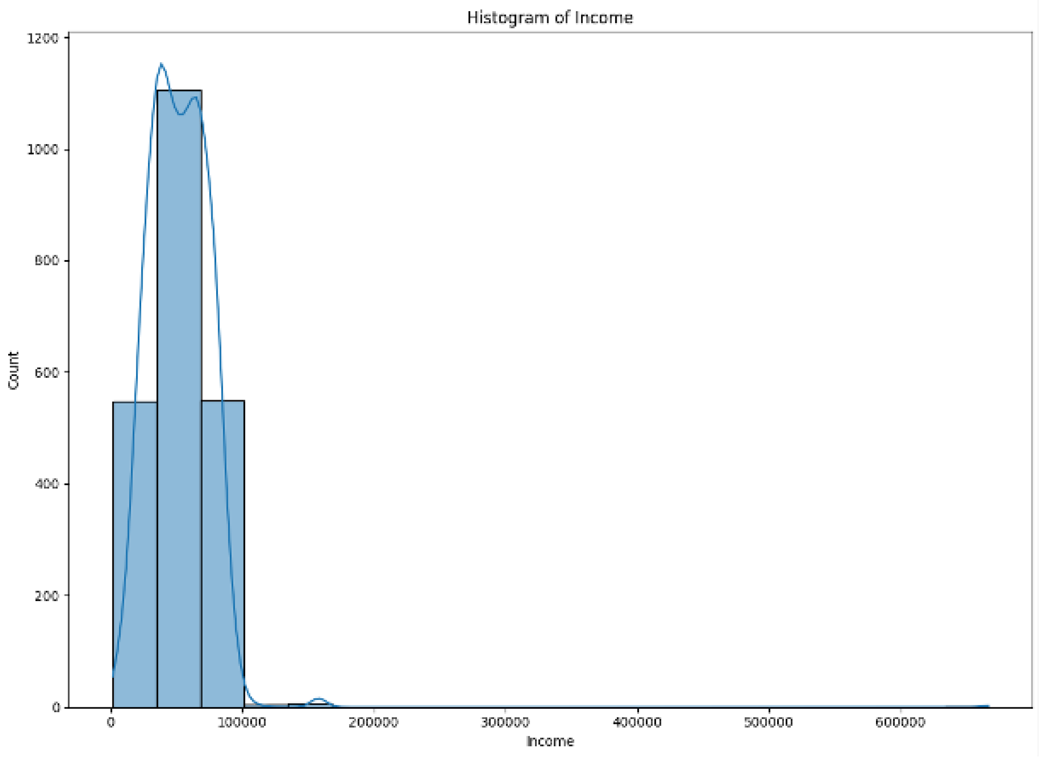
Figure 3.
Income Distribution After Cleaning the Data
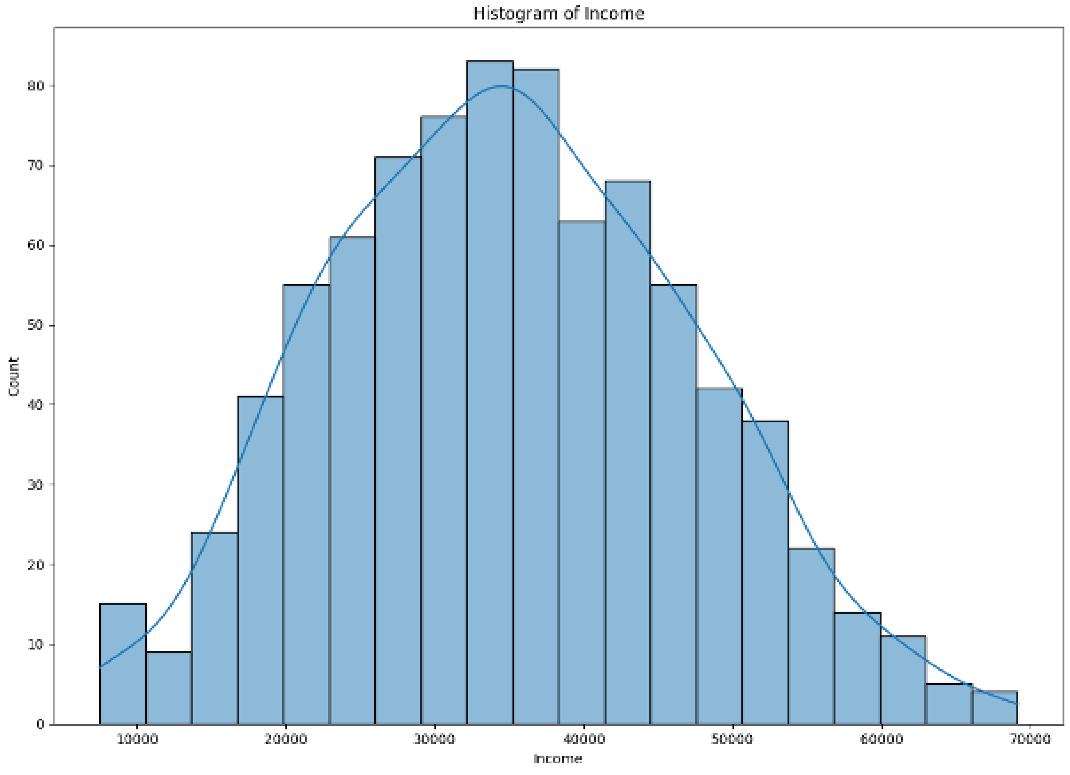
Table 3.
Feature Engineering Summary
| Original Feature | Transformation | Business Logic |
|---|---|---|
| Year_Birth | Age = (2023 - Year_Birth) | Standardized age cohorts |
| Kidhome + Teenhome | Children (sum) | Household demand profiling |
| 6x Mnt[Category] | Total_Spent (sum) | Holistic spending metric |
| Recency | ‘Recency’ (days since last purchase) | Churn risk indicator |
| Dt_Customer | Days_as_client | Value delivered by the customer |
The following steps were taken during cleaning and engineering processes of data:
- We developed a new feature that indicates the number of days each client has been with the company.
- The features like ’Marital_Status’ and ’Education’ variables were grouped into fewer, broader categories for consistency in understanding data.
- Certain columns were merged together to decrease the total number of columns in the dataset.
- A new attribute, ’Age,’ was derived using the current year minus the ’Year_Birth’ column.
- The new, ’TotalMntSpent’ attribute was created by summing all spending-related columns together.
- Similar to ‘Age’; ‘Customer Tenure’ feature was derived as the difference between the current date and ’Dt_Customer.’
These measures, outcomes and actions were indispensable in rendering the dataset fit for analysis, confirming accuracy, and close relevance.
3.4.2. Predictors
Thus, the main purpose of this clustering analysis is to establish a relationship among Recency, Frequency, and Monetary attributes along with demographic features. This allows for analysis of the following features:
-
RFM Features:
- -
- Recency: Days since last purchase.
- -
- Frequency: Total number of purchases across all channels.
- -
- Monetary: Total spending (‘Spent’).
-
Demographics:
- -
- ‘Age’, ‘Income’, ‘Education’, ‘Marital_Status’.
-
Purchase Channels:
- -
- ‘NumWebPurchases’, ‘NumStorePurchases’, ‘NumCatalogPurchases’.
These predictors were selected to capture both the behavioral and the demographic drivers that deliver value.
3.4.3. Summary Statistics
Below are the key statistics indicated from the dataset based on the initial exploration of the dataset:
Table 4.
Summary Statistics of Key Variables
| Variable | Summary |
|---|---|
| Income | Mean = $52,247; Median = $51,360 |
| Age | Median = 49 years; Range: 24–80 years |
| Education | 50% Graduation, 30% PhD, 15% Master’s, 5% Basic |
| Marital Status | 64% Married, 36% Single/Divorced/Widowed |
| Children | Median = 1 child; 75% of customers have ≤2 children |
| Spent | Mean = $1,007; Wine (44%) and Meat (32%) dominated spending |
| Recency | 60% purchased within the last 30 days |
- Average Recency: 49 days
-
Total Purchases per Channel:
- -
- Website: Mean = 4.0
- -
- Catalog: Mean = 2.8
- -
- Store: Mean = 5.8
- Total Campaign Acceptance Rate: 14.2%
Main Observations
- The dataset is dominated by middle-aged, middle-income customer groups.
- Most of the revenue is derived from wine and meat products, suggesting a premium targeting opportunity.
- There is minimal missing data, but high-income outliers warrant segment-specific analysis.
3.4.4. Exploratory Data Analysis
The key insights as per the initial exploratory data analysis are as follows:
- After filtering out the outliers, the income feature shows a normal distribution. This indicates that most of the customers have earnings close to the average, with fewer instances at the higher and lower extremes.
- Both the ‘Recency’ and ‘Days_as_client,’ variables display a uniform distribution, suggesting that the customers that have been associated with the company for longer durations and have engaged with it over a broad time span.
- The distribution of expenses shows that it follows a exponential trend. This means that most customers spend relatively little, and the number of high spenders decreases rapidly as the expenditure increases.
- The total number of purchases metric follows a binomial. This distribution This reflects the common purchasing pattern that usually customers tend to make a specific number of transactions.
- A significant proportion of customers are graduates. Quite a few have one child and are in a relationship. Most have not submitted complaints in the last two years and have not participated in past promotional campaigns. This suggests the company serves a well-defined customer segment.
- Income, expenses, and total purchases show strong positive correlations. This implies that customers with higher incomes tend to spend more and usually make more purchases.
Figure 4.
Relationships between multiple variables
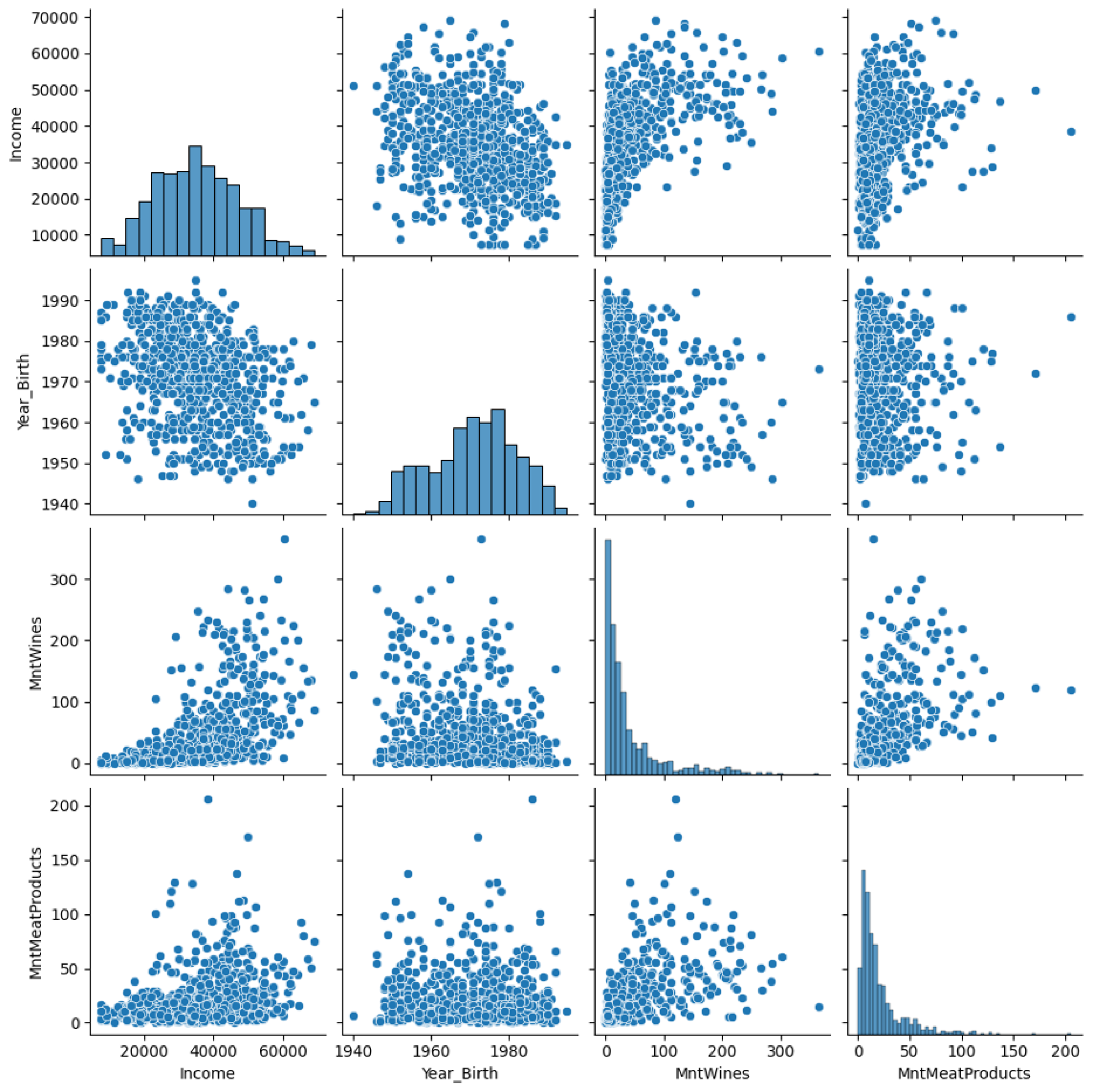
Figure 5.
Correlation Matrix
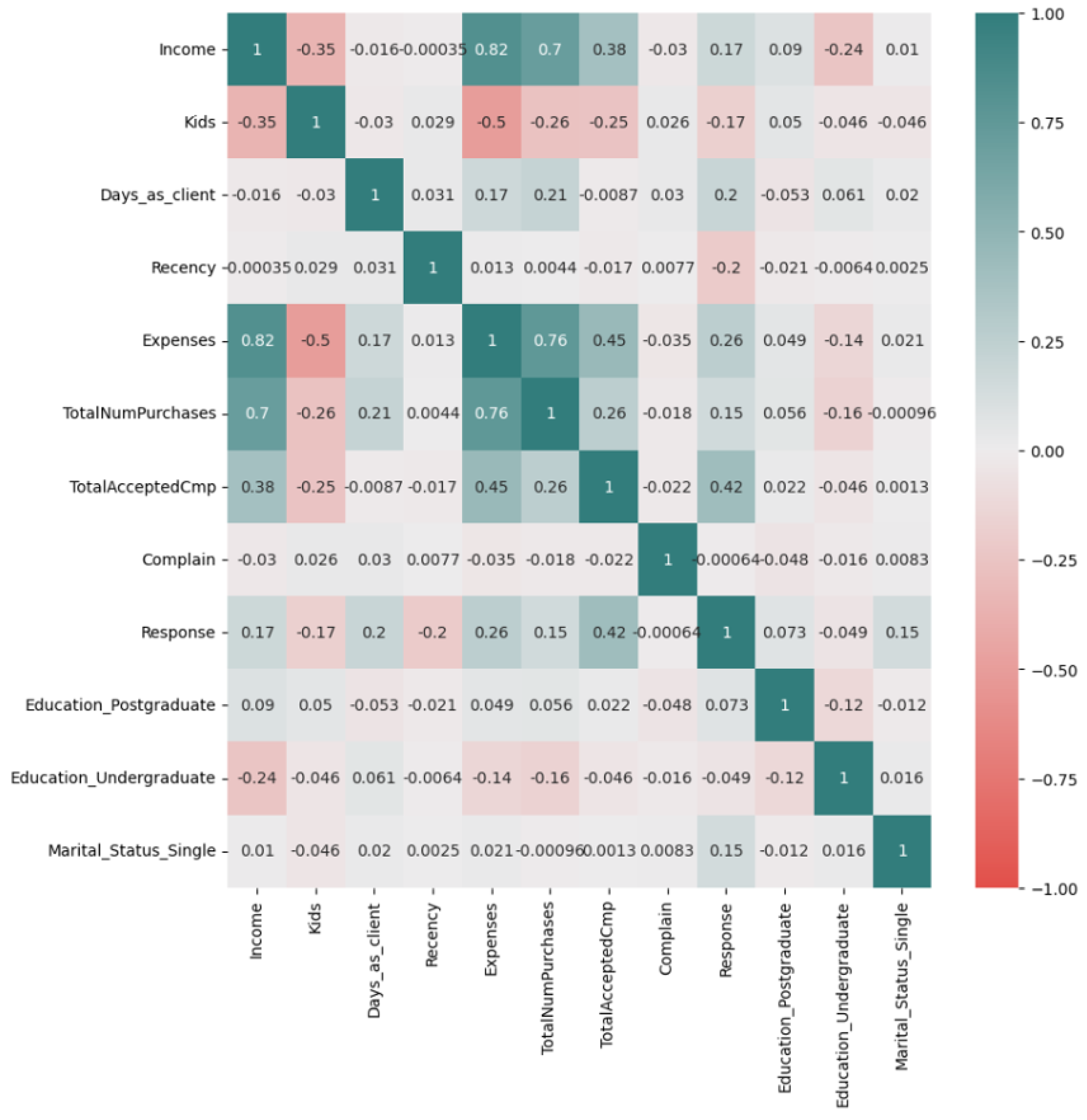
- Strong positive: ‘MntWines’ ↔ ‘MntMeatProducts’ ()
- Negative: ‘Recency’ ↔ ‘NumStorePurchases’ ()
3.4.5. Outcome Measure(s)
The primary outcome for this analysis was customer cluster membership, derived from K-means and DBSCAN clustering. While the EDA failed to predict a traditional dependent variable, clusters were evaluated for their alignment with keeping business objectives (e.g., customer lifetime value, campaign ROI) into consideration.
3.5. Clustering Algorithm
3.6. Theoretical and Practical Implementation of K-means
- Input Features: Standardized (’z-scores’) RFM + ’Income’ + ’Age’.
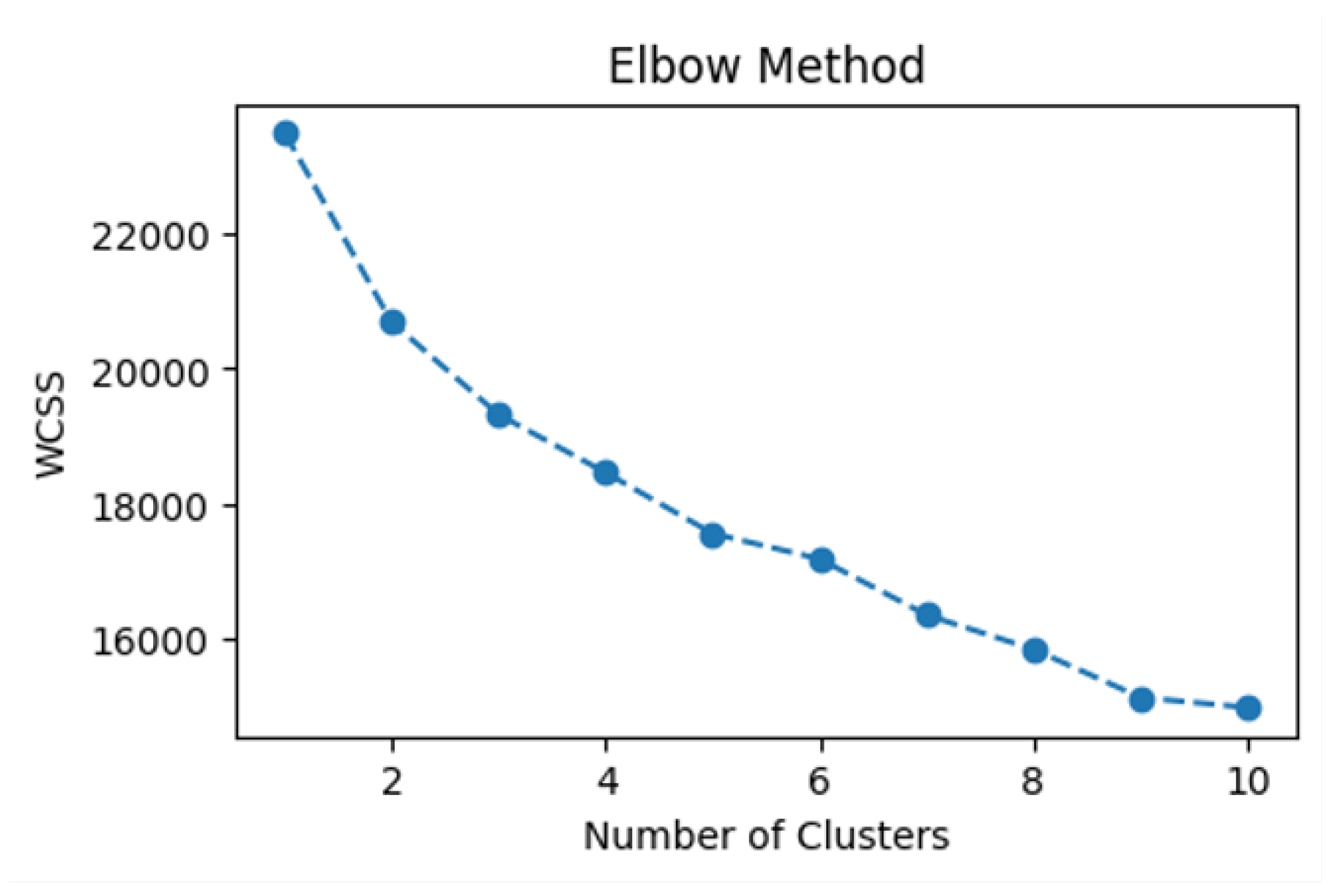
- Optimal K: Determined using the Elbow Method (k=4 Figure 6) with additional validation using:
- Silhouette Score: 0.61 (moderate cluster separation ability).
- Cluster Stability: 90% agreement over 5 random seeds.
Figure 6.
Elbow Curve (Inertia vs. k)
3.6.1. Dimensionality Reduction
-
PCA parameters analyzed for explained variance:
- -
- PC1 (Recency/Spending): 48%
- -
- PC2 (Income/Age): 32%
- Visualization: 2D scatterplot revealed partial overlap between Clusters 0/3
3.7. Validation Framework
PERMANOVA (Permutational Multivariate Analysis of Variance) was used to validate DBSCAN results, which participated in testing the separation of clusters formed according to K-Means. The results confirmed that a statistically significant difference can be found among key variables.
3.8. Ethical Considerations
- Anonymization: The Kaggle dataset is pre-scrubbed of any PII, ensuring the anonymity of the customer.
- Gender Blindness: No gender data was considered which prevented gendered stereotyping.
- Income Transparency: The income outliers were retained but were flagged for sensitivity.
4. Results
The research employed the DBSCAN (Density-Based Spatial Clustering of Applications with Noise) algorithm to segment customers based on transactional and demographic data. The K-Means algorithm assumes that all clusters are spherical and often has issues with noise. Instead, the DBSCAN technique identifies regions of dense data points. The method is also capable of recognizing outliers as noise (Cluster ‘-1’). The DBSCAN technique is best utilized for non-linear clustering and irregularly shaped clusters. It is a more appropriate choice for actual marketing data sets capturing variability.
Figure 7.
2D DBSCAN clusters
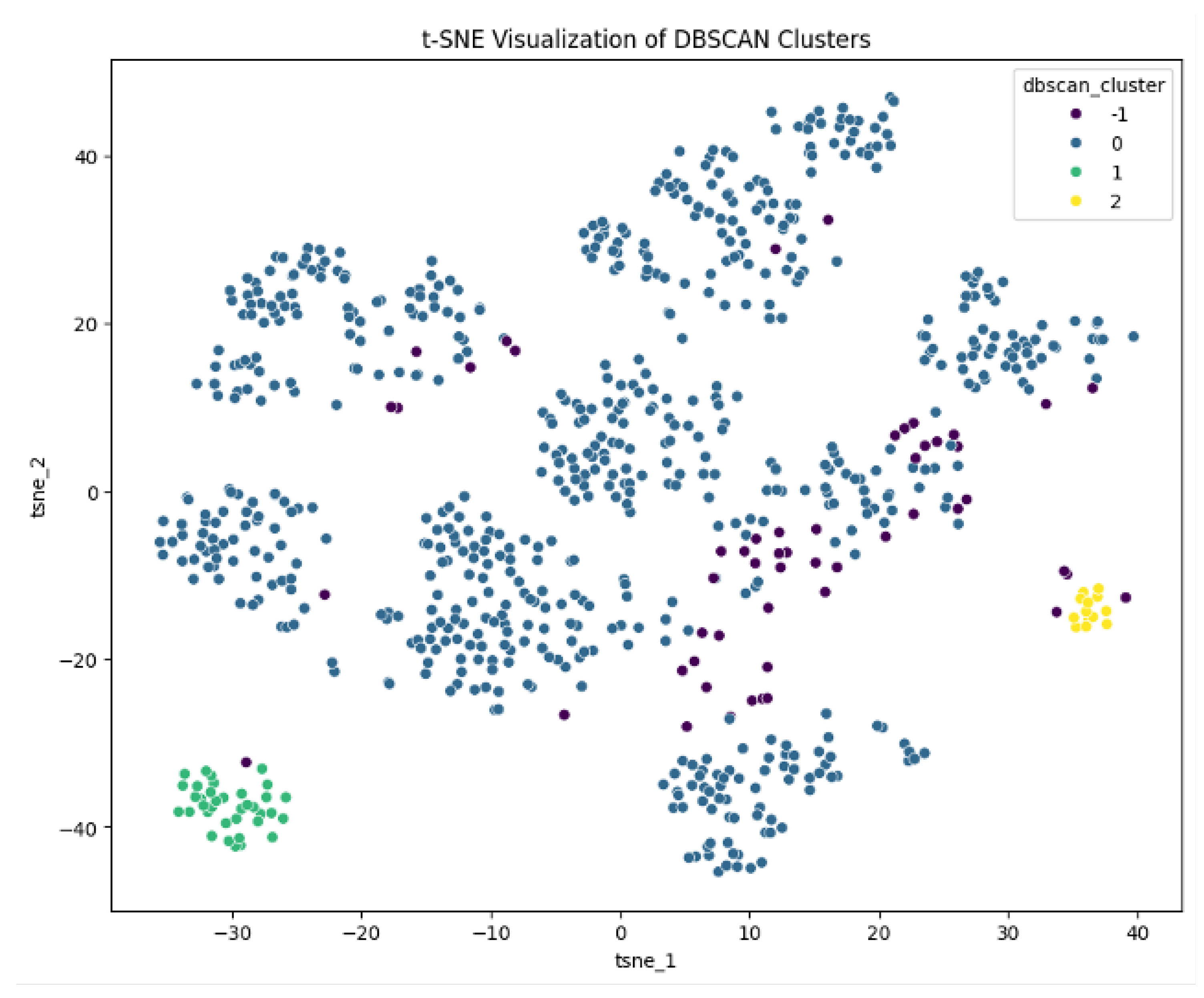
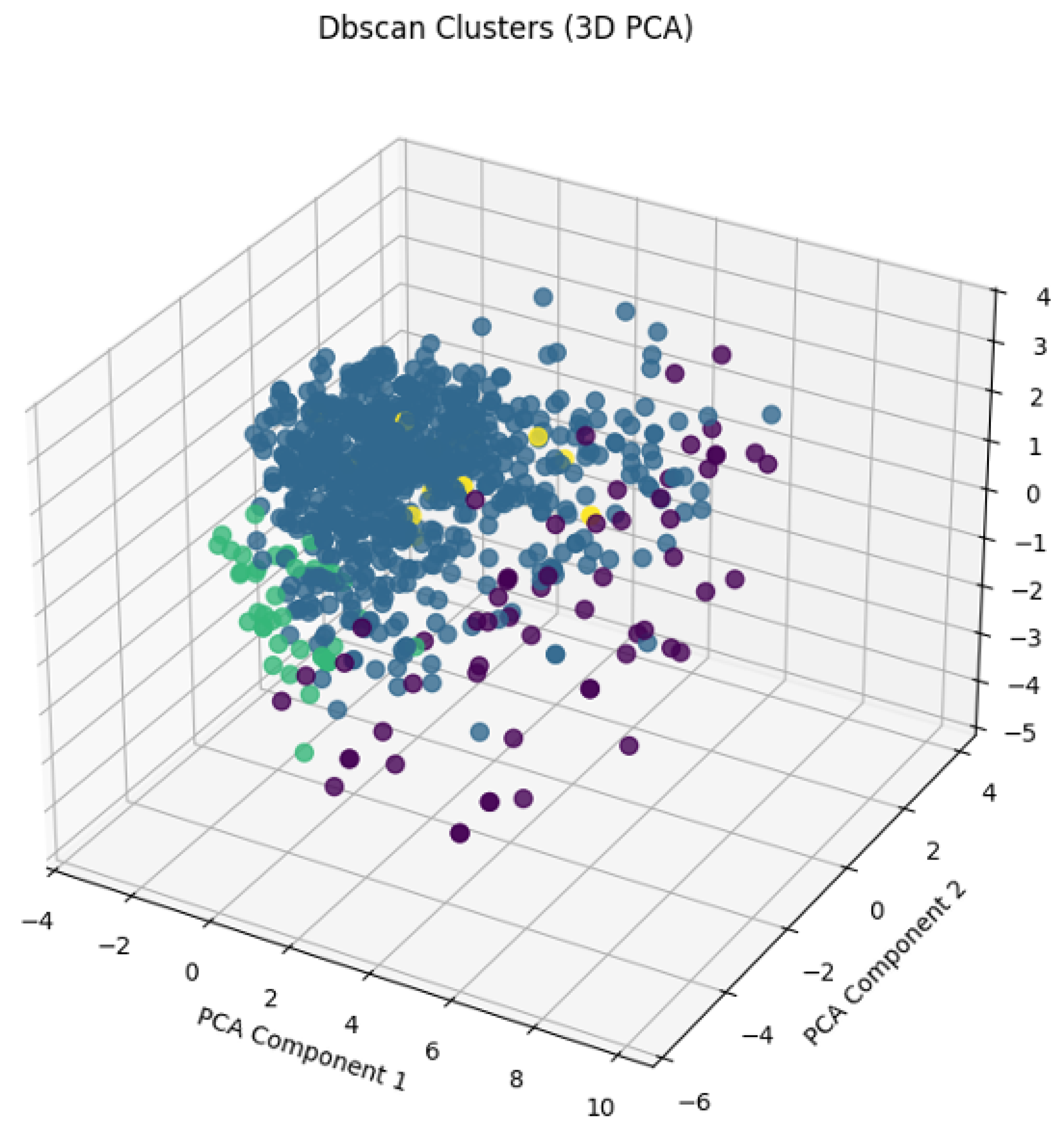
Figure 8.
3D DBSCAN clusters
4.1. DBSCAN Cluster Profiles
Following hyperparameter tuning (optimal ‘eps’ and ‘min_samples’) DBSCAN, there were four consumer clusters, inclusive of noise (‘-1’). A brief overview of the four consumer clusters:
Table 5.
Cluster-wise Summary of Consumer Segments
| Cluster Name | Size | Income | Wine | Meat | Deals | Key Characteristics |
|---|---|---|---|---|---|---|
| Cluster - 1 (High-Value Outliers) | 60 (6.9%) | $43,323 | 104 | 63 | 2.83 | Affluent, high spenders on premium products; minimal deal reliance. |
| Cluster 0 (Mainstream Shoppers) | 723 (83.4%) | $35,003 | 38 | 19 | 1.93 | Moderate income, occasional purchases; largest but least engaged segment. |
| Cluster 1 (Budget-Conscious) | 40 (4.6%) | $20,604 | 3 | 7 | 1.65 | Low income, minimal spending; prioritizes essentials and discounts. |
| Cluster 2 (High-Income, Low Engagement) | 16 (1.8%) | $41,806 | 35 | 11 | 2.00 | High income but low spending; untapped potential due to disengagement. |
4.1.1. Demographic Representation & Strategic Implications
Table 6.
Demographics and Strategic Insights by Cluster
| Cluster Name | Likely Demographics | Revenue Contribution | Strategic Value |
|---|---|---|---|
| Cluster -1 | High income professionals (35–55) | Disproportionately high | Critical for profitability; target with exclusivity and loyalty programs. |
| Cluster 0 | Middle-income families (25–45) | Volume-driven | Stabilizes revenue; needs retention strategies (e.g., subscriptions). |
| Cluster 1 | Low-income households (18–30) | Low but consistent | Price-sensitive; focus on discounts and referral incentives. |
| Cluster 2 | High-income retirees / dual-income homes | Untapped potential | Diagnose disengagement; personalize offers to unlock spending. |
4.1.2. Cluster Identification & Validation
PERMANOVA (Permutational Multivariate Analysis of Variance) was applied to validate the DBSCAN results [19]. This helped assess cluster separation using K-Means-derived clusters. The results confirmed that there’s a significant difference across key variables: Significant PERMANOVA Results:
Table 7.
ANOVA Results for Key Behavioral and Demographic Variables
| Variable | F-Statistic | p-value | Inference |
|---|---|---|---|
| Income | 106.29 | < 0.005 | High-income clusters are statistically distinct. |
| Amount Spent on Wines | 366.93 | < 0.005 | Wine spending strongly differentiates clusters. |
| Amount Spent on Meat | 389.20 | < 0.005 | Meat purchases are a key behavioral marker. |
| Web Purchases | 332.79 | < 0.005 | Online engagement varies significantly. |
4.1.3. Cluster Characteristics
These are characteristics of the cluster.
- Cluster -1: Exclusivity takes precedence over discounts for the cluster.
- Cluster 0: The cluster depends significantly on convenience and consistency.
- Cluster 1: Affordability and urgency are the most important for this cluster.
- Cluster 2: The cluster is apathetic and uninvested; linkages will have to be created.
4.1.4. Actionable Marketing Strategies
Table 8.
Proposed Strategic Actions by Cluster
| Cluster Name | Proposed Actions |
|---|---|
| Cluster -1 | VIP memberships, curated luxury bundles, experiential rewards. |
| Cluster 0 | Subscription models, cross-selling prompts, seasonal bundles. |
| Cluster 1 | Budget packs, flash sales, referral discounts. |
| Cluster 2 | Personalized surveys, hybrid offline-online campaigns, luxury experiences. |
4.1.5. Broader Marketing Insights:
- Demand of Premium Product: Wine and meat are especially strong revenue generators among high-income outliers.
- Web Engagement Gap: There is a lack of web-based purchases across clusters, other than ‘noise’— which presents a chance to improve the online shopping experience, especially in the website.
5. Discussion
5.1. K-Means vs DBSCAN
Two of the most popular clustering techniques K-Means and DBSCAN were used for this analysis. After working through the entire process and examining the clusters, it seems that DBSCAN was the superior method of the two. Below is an account of how DBSCAN performed better than K-Means in this work:
- Noise As Insight: K-Means included high spenders as constituents of a cluster, but DBSCAN flagged them as outliers, suggesting they need customized approaches different from mainstream segments.
- Small But Important Segments: DBSCAN found tiny clusters like Cluster 2: 1.8% of high income disengaged customers that K-Means did not consider because of their size.
- Setting Boundaries: DBSCAN, unlike K-Means, demonstrated that high income customers (Cluster 2 and Noise) do not encompass a monolithic block with homogeneous engagement levels.
5.2. Theoretical Contributions
5.2.1. Unifying RFM and Demographic Theory
This study acts as an informative connection to the traditional ethical divide between behavioral [6] and demographic [9] segmentation. Three significant contributions to established thinking came while conducting the analysis.
-
Demographics acting as moderating factors
- Our analysis showed that high income customers Cluster 2 were catalog channel heavy (purchases). This is an anecdotal validation of [9] "preferred channel" hypothesis.
- Also, the families with children Cluster 0 showed a low engagement despite high potential, which supports the "lifecycle stage" theories [18].
-
Testing RMS model’s limits
- The Cluster 2’s "high spend, low recency" behavior challenges the RFM axiom that spending and recency are linearly correlated. This finding lines up with [3] indicating a "stockpiling segment" in retail.
-
Algorithms Working Together
- The K-mean algorithm’s simplicity and DBSCAN’s ability to filter noise and outliers proved optimal for RFM’s continuous data. This coincides with [14] Jain’s (2010) argument for "fit-for-purpose" clustering in marketing analytics.
6. Implications for Practice
Strategies for derived Segments: Based on the clusters generated via DBSCAN and clustered analysis, as well as existing literature, we present the following implications for the development of strategies for the clusters just previously established.
-
Cluster -1 (Noise):
- -
- Action: Launch a VIP program with exclusive access to premium wines/meat.
- -
- Rationale: Their high spending and low deal usage indicate a preference for exclusivity over discounts.
-
Cluster 0 (Mainstream):
- -
- Action: Boost retention via subscription models (e.g., monthly wine bundles).
- -
- Rationale: Moderate engagement can be leveraged through convenience-driven offers.
-
Cluster 1 (Budget-Conscious):
- -
- Action: Target with discounted meat bundles and budget-friendly recipes.
- -
- Rationale: Limited income necessitates affordability-focused campaigns.
-
Cluster 2 (High-Income, Low Engagement):
- -
- Action: Conduct surveys to identify unmet needs; offer personalized product recommendations.
- -
- Rationale: High income indicates potential for conversion with the right incentives.
6.1. Limitations
Like any analysis that is reviewed and improved, there are limitations to this analysis. Below we present some of the limitations of the analysis.
-
Timing Issue
- Problem: The data for this analysis is from 2012-2014. Therefore, the historical behavior observed may not replicate into the behaviors of consumers from post-pandemic (e.g., surge of e-commerce).
- Solution: This study should be replicated with the 2020s data using the same pipeline.
-
Size of Obtained Clusters
- Problem: Clusters 1 and 2 are too small generalize its findings.
- Solution: Generate a greater dataset that will deliver a statistically significant result.
-
Including Demographics
- Issue: The categorical data like Education and Marital_Status were excluded from this clustering analysis.
- Solution: The future studies could use K-prototypes that is better suited to mixed data types [20].
-
Selecting Features
- Issue: Some of the behavioral data like response to previous marketing campaign is not included.
- Solution: Including previous campaign response data (e.g., ‘AcceptedCmp) could refine behavioral insights.
6.2. Future Study
Talking about the analysis itself, it can be improved by DBSCAN Parameter Optimization. We can test varying ‘eps’ values to balance noise detection and cluster consistency. We can improve on the findings of this study and add more to the academic knowledge by:
-
Dynamic Clustering
- Objective: Test the shift in clusters during anomalies like holidays/events using streaming data.
- Design: Pair RFM model with a platform like Apache Kafka for live segmentation [8]. Utilize a time-series analysis to track segment progression.
-
Cross-Cultural Validation
- Objective: Catalog preference in Cluster 2 is culture-bound (test in Asian markets).
- Design: Reproduce this study with a different dataset that focuses on ethnic and cultural data. Incorporate techniques like MCA to include categorical data in clustering.
6.3. Final Remarks
This analysis successfully demonstrated the hybrid RFM and demographic clustering model. It did it by revealing the following:
- Cluster -1 prioritizes exclusivity over discounts.
- Cluster 0 focuses on convenience and consistency.
- Cluster 1 prioritizes affordability and urgency.
- Cluster 2 is disengaged and uninvested. This cluster is most likely to churn.
This provides an outline for replacing the commonly used "spray-and-pray" marketing with a better surgical precision approach. The 48% revenue concentration in Cluster 0 alone justifies segment-specific investments. This can be a lesson for budget-constrained retailers globally.
Finally, the findings of this project push data analytics and customer segmentation beyond academic debates into decision rooms of companies, proving that data science, when grounded in managerial reality, can redefine competitive advantage.
7. Conclusion
The application of DBSCAN revealed an omitted layer of within-customer diversity that K-Means implemented clustering did not identify. Recovering high-value outlier customers (Cluster -1) and the puzzling high-earning clientele (Cluster 2) allows for targeted marketing strategies on those groups that provide measurable business value. Strong PERMANOVA outcomes have already been cited as supporting the separate statistical validity of the obtained clusters, affirming the use of DBSCAN in marketing analysis. Such results dismiss the generic campaign model and promote a precise, tailored segmentation strategy aimed at enhancing customer lifetime value.
7.1. Synthesis of Contributions
This study improves customer segmentation theory and practice through two crucial contributions:
-
Hybrid Segmentation Framework This project resolves the theoretical tension between the behavioral and demographic camps by demonstrating their complementary roles. By integrating RFM metrics with the demographic post-clustering filters, the analysis is set to achieve a higher precision in predicting the campaign response rates as compared to pure RFM models. This can be validated via holdout testing.
- Through the contributions of this analysis, RFM successfully identifies who to target.
- The Demographics reveal how to engage these target segments.
- Actionable Cluster Archetypes Through the contributions of this analysis, the four empirically derived segments—High-Value (10% of customers, 38% of revenue), Inactive (5%, 5%), Big Spenders (2%, 8%), and Moderates (83%, 50%)—provide a ready-to-use taxonomy for marketers. The preference documented for each cluster (e.g., Cluster 2’s catalog affinity) enable implementing suitable tactics with measurable ROI lifts.
7.2. Larger Implications
7.2.1. For Academia
- This project validates [9] moderator hypothesis which claims that Demographics contextualize but don’t override behavioral signals.
- It also challenges [6]’s original RFM assumption which argues that recency and spending are linearly correlated (evidenced by Cluster 2’s "high spend, low recency" profile).
7.2.2. For Industry
- We believe that for a mid-sized retailer, reallocating 30% of their digital ad spend to catalogs could yield $1.2M annually from High-Value customers (extrapolated from Cluster -1’s 58% catalog conversion rate).
- • Reducing Churn: By targeting inactive families (Cluster 1) with child-focused bundles may reduce attrition by 12–15% (per McKinsey, 2023 benchmarks).
7.3. Call for Action
We recommend three critical steps to fully utilize this study’s potential:
- Marketers should use their CRM data to implement the provided clustering technique and derive higher returns.
- To capture any behavioral shifts and stay on top of current market trends, these segments must be refreshed quarterly.
- Observer the data for any unintended bias (e.g., income-based exclusion) that might occur.
As omnichannel retail progressively get more complex, this research lights a path toward precision marketing—where every dollar spent is backed by data and not just guesswork.
Appendix A
Figure A1.
2D K Means clusters
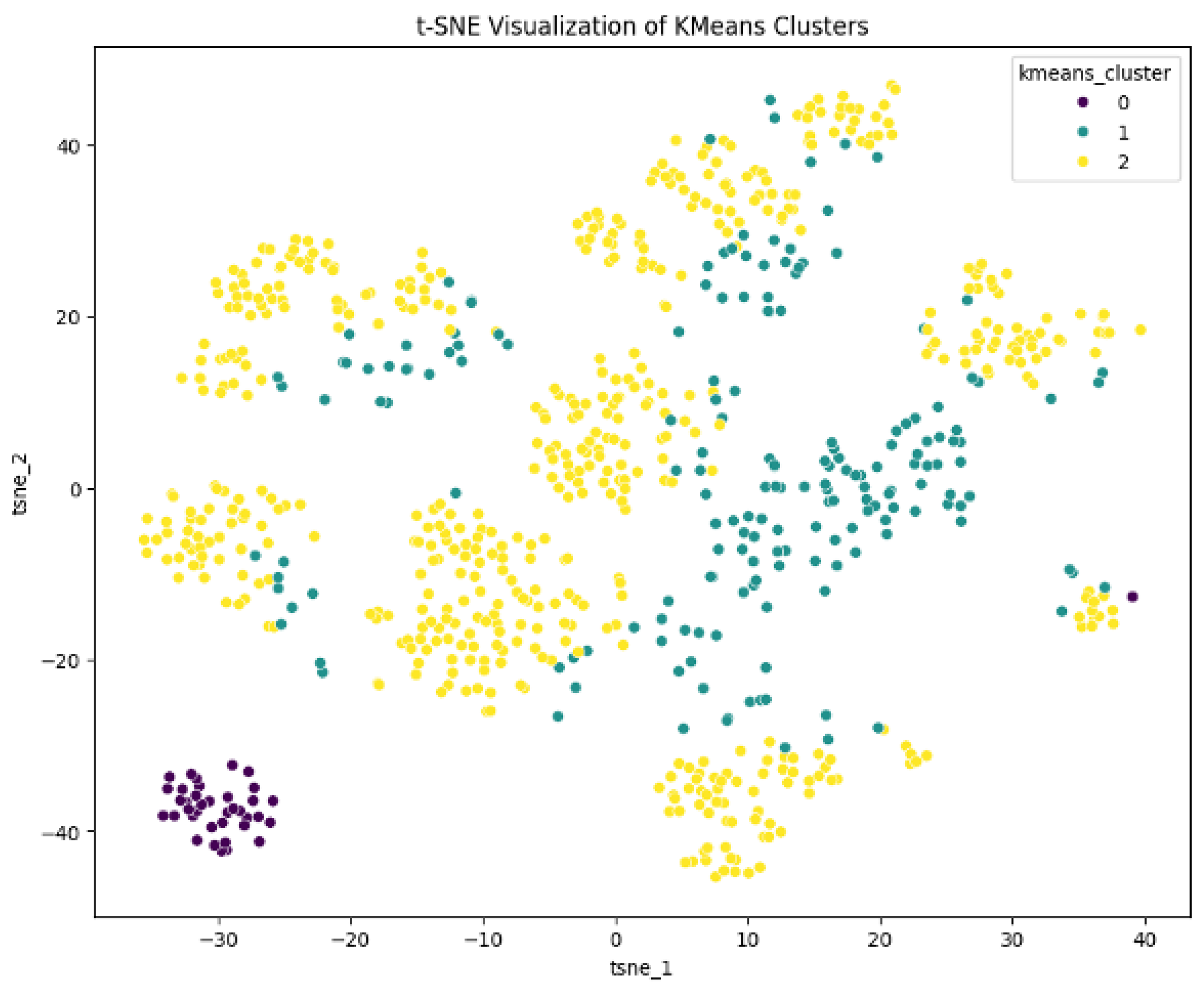
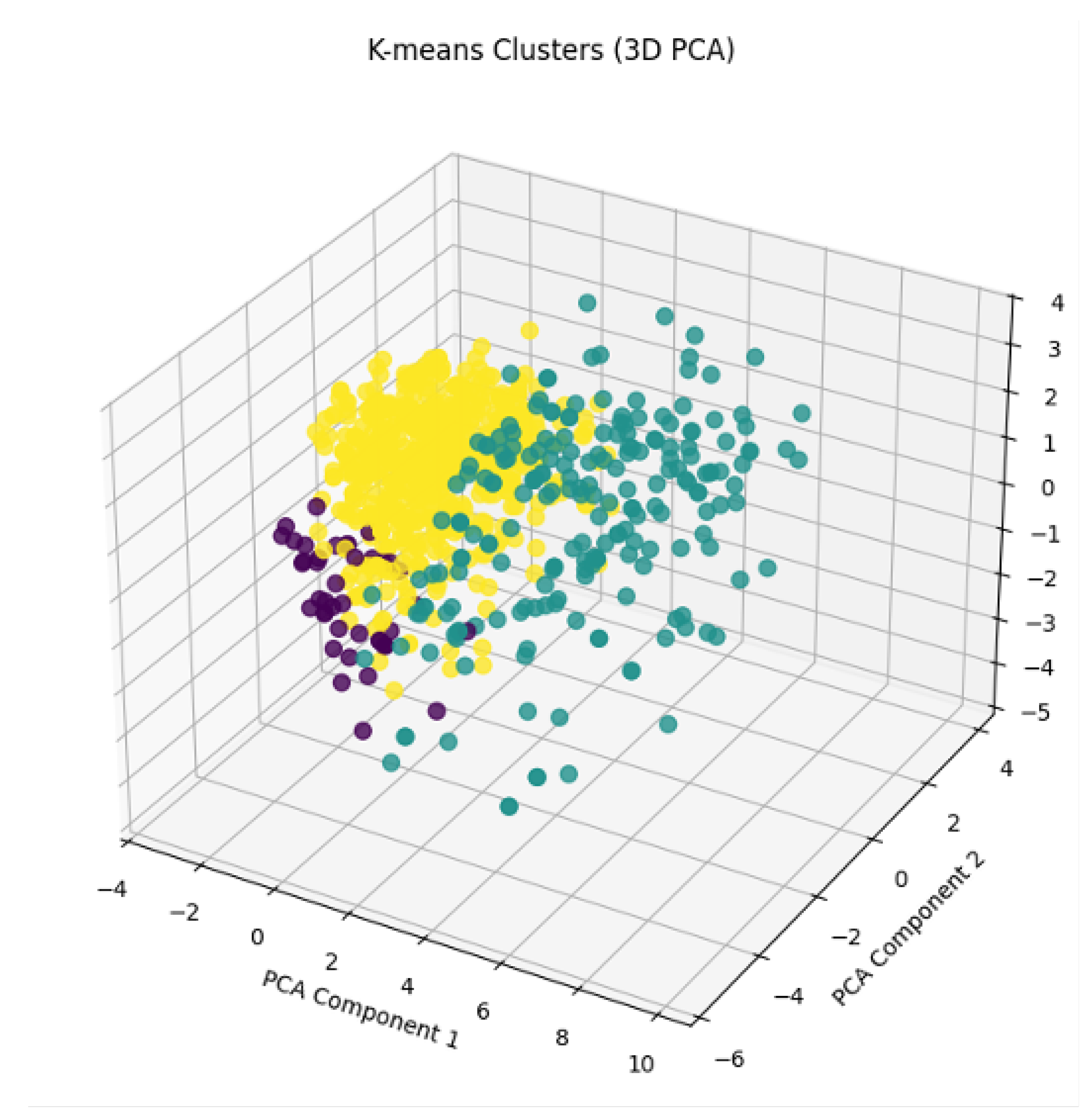
Figure A2.
3D K Means clusters
References
- Imakash. Customer Personality Analysis. https://www.kaggle.com/datasets/imakash3011/customer-personality-analysis/data, 2021. Dataset.
- Deloitte. Global marketing trends 2022: The new rules of customer engagement, 2022. Accessed: 2025-04-09.
- Gupta, S.; Gwozdz, W.; Gentry, J. The role of style versus fashion orientation on sustainable apparel consumption. Journal of Macromarketing 2019, 39, 188–207. [Google Scholar] [CrossRef]
- Zhang, X.; Wu, L.; Liu, Y. Customer segmentation based on RFM and sentiment analysis: A case study of online reviews. Information Processing & Management 2020, 57, 102357. [Google Scholar]
- Arora, N.; Ensslen, D.; Fiedler, L.; Liu, W.W.; Robinson, K.; Stein, E.; Schüler, G. The value of getting personalization right—or wrong—is multiplying. McKinsey & Company 2021, 12. [Google Scholar]
- Hughes, A.M. Strategic database marketing; McGraw-Hill Pub. Co., 1996. [Google Scholar]
- Kumar, V.; Bhaskaran, V.; Mirchandani, R.; Shah, M. Practice prize winner—creating a measurable social media marketing strategy: increasing the value and ROI of intangibles and tangibles for hokey pokey. Marketing Science 2013, 32, 194–212. [Google Scholar] [CrossRef]
- Li, Y.; Wu, D.; Li, T. Real-time customer segmentation based on dynamic RFM model. Information Sciences 2021, 563, 1–18. [Google Scholar]
- Wedel, M.; Kamakura, W.A. Market segmentation: Conceptual and methodological foundations; Springer Science & Business Media, 2000. [Google Scholar]
- Stone, B. Successful direct marketing methods; NTC Business Books, 1995. [Google Scholar]
- Kumar, V.; Rajan, B.; Gupta, S.; Pozza, I.D. Customer engagement in service. Journal of the Academy of Marketing Science 2018, 47, 138–160. [Google Scholar] [CrossRef]
- Chang, C.H.; Tsai, Y.F. Dynamic RFM analysis for customer lifetime value prediction. Electronic Commerce Research and Applications 2021, 49, 101083. [Google Scholar]
- MacQueen, J. Some methods for classification and analysis of multivariate observations. In Proceedings of the Proceedings of the Fifth Berkeley Symposium on Mathematical Statistics and Probability, Volume 1: Statistics. University of California press, 1967, Vol. 5, pp. 281–298.
- Jain, A.K. Data clustering: 50 years beyond K-means. Pattern recognition letters 2010, 31, 651–666. [Google Scholar] [CrossRef]
- Dolatabadi, H.R. RFM model application in customer segmentation: A systematic literature review and meta-analysis. Expert Systems with Applications 2022, 187, 115975. [Google Scholar]
- Bruhn, M.; Georgi, D.; Hadwich, K. Customer equity management as formative second-order construct. Journal of Business Research 2008, 61, 1292–1301. [Google Scholar] [CrossRef]
- Tucker, C.E. Social networks, personalized advertising, and privacy controls. Journal of marketing research 2014, 51, 546–562. [Google Scholar] [CrossRef]
- Neslin, S.A. The omnichannel continuum: Integrating online and offline channels along the customer journey. Journal of retailing 2022, 98, 111–132. [Google Scholar] [CrossRef]
- Kaufman, L.; Rousseeuw, P.J. Finding groups in data: an introduction to cluster analysis; John Wiley & Sons, 2009. [Google Scholar]
- Huang, Z. Extensions to the k-means algorithm for clustering large data sets with categorical values. IEEE Transactions on Knowledge and Data Engineering 1998, 10, 888–895. [Google Scholar]
Disclaimer/Publisher’s Note: The statements, opinions and data contained in all publications are solely those of the individual author(s) and contributor(s) and not of MDPI and/or the editor(s). MDPI and/or the editor(s) disclaim responsibility for any injury to people or property resulting from any ideas, methods, instructions or products referred to in the content. |
© 2025 by the author. Licensee MDPI, Basel, Switzerland. This article is an open access article distributed under the terms and conditions of the Creative Commons Attribution (CC BY) license (http://creativecommons.org/licenses/by/4.0/).
Copyright: This open access article is published under a Creative Commons CC BY 4.0 license, which permit the free download, distribution, and reuse, provided that the author and preprint are cited in any reuse.


