Submitted:
16 April 2025
Posted:
16 April 2025
You are already at the latest version
Abstract
The convergence order of Jarratt-type methods for solving nonlinear equations are obtained without using the Taylor expansion. We use assumptions on the derivatives of the involved operator up to second order only contrary to the earlier studies. The proof provided in this paper does not depend on the Taylor series expansion which in turn reduces assumptions on the higher order derivatives of the involved operator and increases the applicability of these methods. The applicability of the method is further extended using the concept of generalized condition in the local convergence and majorizing sequences in the semi-local analysis. Numerical examples and Basins of attractions of the methods are provided in this study.
Keywords:
taylor expansion
; order of convergence(OC)
; jarratt method
; fréchet derivative
1. Introduction
Several real-world problems can be mathematically modelled as an equation of the form
where is a nonlinear operator mapping between the Banach spaces X and Y and E is open convex set in One of the most challenging problems appearing in real-world is to determine the solution of (1). Iterative methods are an alternate attractive technique to approximate solutions of nonlinear equations as obtaining the exact solution to these nonlinear equations becomes difficult. One of the most extensively used quadratically convergent iterative method is Newton’s method as it converges rapidly from any sufficiently good initial guess. Even though this method provides a good convergence rate, the need to compute and invert the derivative of the given operator function in each of the iterative step, limits the applicability of these method. To overcome this several Newton-like methods are available in the literature [1,3,5,13,19]. One such successful attempt was made by Ren et al., in [18] providing iterative method (see(2)) of order six. Recall [10] that a sequence in X with is said to be convergent of order , if there exist a nonzero constant C such that
Previous studies primarily used Taylor expansion to determine the order of convergence(OC), which necessitates the existence of higher-order derivatives. An alternative method involves employing the computational order of convergence (COC) [23], defined as:
where are three consecutive iterates near root or the approximate computational order of convergence (ACOC) defined as:
where are four consecutive iterates near root , to obtain the OC.
The limitation of COC and ACOC for iterative methods lies in their susceptibility to the oscillating behavior of approximations and slow convergence during early iterations [17]. As a result, COC and ACOC do not accurately reflect the true OC.
In [18], Taylor’s expansion is used to achieve a sixth-order convergence, but the analysis requires conditions on the derivatives of up to the seventh order. These assumptions restrict the applicability of the method (2) to problems involving operators that are differentiable at least seven times.
In this article, we initially determine the OC of the method (refer to [9,13]) defined for all as follows:
where X and Y are Banach spaces. The local convergence of certain Jarratt-type methods was analyzed in [2] by relying solely on assumptions about the derivative of order one of . However, the OC was determined using COC and ACOC, which, as previously noted, are not ideal for calculating the convergence order. This raises the question: can we establish a third-order convergence for (3) and a sixth-order convergence for (2) without using assumptions on the higher-order derivatives of or Taylor expansion?
Additionally, we enhance the method to a fifth-order approach, given as follows:
in Section 4.
In Section 2, we establish a third-order convergence for method (3), and in Section 3, we demonstrate a sixth-order convergence for (2), relying on assumptions about the derivatives of up to the second order. Consequently, our analysis broadens the applicability of methods (3), (2), and (4) to problems that could not be addressed using the approaches in [4,14,18,20,21].
In Section 5, we examine the constraints of our approach and propose novel strategies to overcome these limitations for local as well as semi-local convergence scenarios. The convergence conditions are solely tied to the operators involved in the method for both the semi-local and local cases.
2. Order of Convergence(OC) of (3):
The analysis of local convergence relies on the following assumptions:
- (A1)
- &∃ such that
- (A2)
- s such that
- (A3)
- ∃ such thatand
- (A4)
- ∃ such that
Using the constants and , we define continuous nondecreasing functions (CNF) as follows;
and
Given that and as t tends to , it follows that has a smallest positive root in the interval , which we denote by . Define CNF by
and
Since and as , it follows that has a smallest positive root in the interval , which is denoted by .
Let
Then, we have
Throughout the paper, we consider and , for and
Theorem 1.
Assuming (A1)-(A4) are true, the sequence given by (3) with initial value converges to , and the following estimate is valid:
Proof. An inductive argument will be employed for the proof. As a first step, we will demonstrate that the operator is invertible for all belonging to the open ball Note that, by (A1), we have
Therefore, by Banach lemma(BL)on invertible operators, is invertible and by (8), we have
Similarly, one can prove that
Next, by the method (3), we have,
Note that,
For convenience, let In order to prove (7), we rearrange the equation (11) as follows:
Let and Then, by (13), we have
where,
and
Next, we estimate the norms of and Note that,
which is obtained using (A2) and (10)(with ). Note that and using (10) we have,
Therefore,
and hence by (9) (with and ), we have
Therefore, on using (17) in (15) we get,
Next,
Therefore, by (9), (10), (A1) and (A3), we have
By using (9) and (A2), we have
Thus, by (16) and (17), we have
Similarly, we have
So, by using (16) and (17), we have
Next, we shall obtain an estimate for Observe that
Therefore, by (9), (A1)-(A4), we have
Thus, from (14)-(24), we have
Therefore, the iterate because
Simply replace in the preceding arguments by to complete the induction for (7). □
Theorem 2.
The method defined by (3) exhibits a convergence order of 3.
Proof. The proof follows a similar argument to that of Theorem 3 in [6]. However, we include it here for completeness. Let Let q be maximal such that for some
Thus, by (25), we get
Thus convergence order
□
3. Order of Convergence(OC) of (2):
This section examines the OC of method (2). For our analysis we require some more CNF:
Let defined by
and
Given that and and , we can conclude that the equation possesses a smallest positive solution within . This solution is denoted as
Let be CNF defined by
and
Then, and as Therefore has a smallest positive solution in denoted by
Let
Then, for all
Theorem 3.
Assuming (A1)-(A4) are true, the sequence given by (2) with initial value converges to , and the following estimate is valid:
Proof. Adopting the same proof strategy as in Theorem 1, we find that:
Note that by (10) and (A1)
Now since the iterate
□
Theorem 4.
The method defined by (2) exhibits a convergence order of
Proof. Employing a proof strategy analogous to that of Theorem 2.
□
4. Order of Convergence(OC) of (4):
We analyze the OC of method (4) in this section. We require some more CNFs as in previous sections:
Let be CNFs defined by
and
Then, and as Therefore has a smallest positive solution in denoted by
Let
Then, for all
Theorem 5.
Assuming (A1)-(A4) are true, the sequence given by (4) with initial value converges to , and the following estimate is valid:
Proof. In imitation of the proof presented for Theorem 1, we obtain:
Note that by (10) and (A1)
Here, we used the inequality
Now since the iterate
□
Theorem 6.
The method defined by (4) exhibits a convergence order of
Proof. Resembling the proof of Theorem 2.
□
The subsequent result addresses the uniqueness property of the solutions derived from the methods (3), (2), and (4).
Theorem 7.
Suppose Assumption (A1) holds and the equation , has a simple solution . Then, for the equation the only solution in the set is provided that
Proof. Suppose is such that Define the operator Then by Assumption (A1) and (35), we have
So by BL, N is invertible and hence we get from the identity
5. Convergence Under Generalized Conditions
The applicability of method (3) and the method (4) can be extended. Notice that the second condition (A2) can can be violated easily even for simple scalar functions. Define the function
Since and is discontinuous at , condition (A2) is violated in any neighborhood containing 0 and 1. This necessitates a convergence analysis based on generalized conditions and the operators inherent to the methods.
First the local convergence is considered under some conditions. Set
Presume:
- (H1)
- Consider a CNF for which the smallest positive solution to is . Let be the interval .
- (H2)
- Let be the SPS of , where the function is given byfor some CNF
- (H3)
-
The equation has a SPS denoted by where is given byLet
- (H4)
- The equation has a SPS denoted by where is given bywhere
- (H5)
-
The equation has a SPS denoted by here is given byLet
- (H6)
- The equation has a SPS denoted by where is given aswhere
Let
The developed functions and relate to the operators on the method (4).
- (H7)
-
There exist an invertible linear operator L and solving the equation such that for eachNotice that under condition (H1) and (36)Thus is invertible. Let
- (H8)
-
for eachand
- (H9)
The main local analysis for the method (4) follows in the next result.
Theorem 8.
Let the conditions (H1)-(H9) hold. Then, the following assertions are satisfied provided that
and where the functions are provided previously and the radius is defined by the formula (36).
Proof. Let It follows that for each
and
The assertions (37)-(40) are shown by induction. Let but be arbitrary. The condition (H1) and the formula (36) give
Thus, is invertible,
and the iterate exists by the method (4) if Moreover, the first substep gives
Using (36), (44) (for ), (H8), (45) and (46)
Thus, the iterate and the item (38) holds if
The following estimate establishes the invertability of the linear operator and iterate by the second substep of the method (4):
where we used the conditions (H3), (H7), formulas (36), (42) and (37). Hence, by (48)
Moreover, the second substep gives
It follows by (36), (44) (for ), (45), (47), (49) and (50)
Thus, the iterate and for the assertion (39) holds. Next the invertability of the linear operator establishes the existence of the iterate as follows:
so
Then, the last substep of the method (4) gives in turn
Using (36), (H8), (44) (for ), (51), (52) and (53)
Hence, the iterate and the assertion (40) holds for The induction is terminated if replaces in the preceding calculations. Finally, from the estimate
where It follows and the iterate
□
The isolation of the solution is discussed in the next result.
Proposition 1.
Suppose: there exists a solution for some the condition (H7) holds in the ball and there exists such that
Let
Then, the equation is uniquelly solvable by in the region
Proof. Define the linear operator Then, by the condition (H7) in the ball and (56)
Hence, follows from the identity □
Remark 1.
A analogous approach is followed in the semi-local analysis but the role of is exchanged by and that of function and by and respectively which are developed below.
Suppose:
- (e1)
-
There exists CNF such that the equation has a SPS denoted bySet Let be a CNF. Define the sequence for and each byand
- (e2)
-
There exists such that for eachIt follows that and there exists such thatThe functions and are connected to the operators on the method (4).
- (e3)
-
There exists such thatLet Notice that (e1) and (e3) imply that the linear operator is invertible. Let
- (e4)
- for each and
- (e5)
As in the local case we obtain in turn and induction the estimates
where
where
and
and
It follows by (57)-(65) that the sequence is complete, since is convergent by the condition (e2). But X is a Banach space. Hence, there exists such that Then, by letting in
we deduce that Finally, notice that for
thus for
Hence, the semi-local result for the method (4) is achieved.
Theorem 9.
Let that the conditions (e1)-(e5) hold. Then, there exists solving the equation Moreover, the following assertions hold
and
The uniqueness property of the solution is specified in the next result.
Proposition 2.
Suppose: There exists a solution of the equation for some the condition (e3) holds in the ball and there exists such that
Let Then, the only possible solution of the equation in the region is
Proof. Let with and the linear operator It follows
Thus, we deduce □
6. Efficiency Indices
There are several measures for comparing iterative methods other than OC, one of them is efficiency of the method. Recall the informational efficiency, introduced by Traub [22] is given by where o is the order of the methods and s is the number of function evaluations. Ostowski [16], introduced a term before Traub called efficiency index or computational efficiency defined as where is the OC of the method and is the number of function evaluations. Thus, the E.I and the C.E of the method (2) are and the E. I and C. E of the method (3) are and and E. I and C. E of the method (4) are and
7. Numerical Example
Example 1.
Consider , , Define function on E for by
Then, the first and second Fréchet derivatives are as follows:
and
Now, we can observe that Thus we get Thus,
Hence , and . With respect to and , we get .
Example 2.
Consider the non-linear integral equation of the Hammerstein-type given by
where H is any function such that
defined on , the space of all continuous functions on the on the interval let Then, we obtain first Fréchet derivatives as
we can observe that is a solution of Then, by applying the conditions we have and . With respect to and , we get and .
In the next example, we compare the iteration and the convergence order of methods (3), (2) and (4) with that of following methods:
8. Basins of Attraction
For an iterative method, the set of all initial points which converges to a solution of an equation is known as Basins of attraction [7,8]. Using the approach of the basins of attractions we obtain the convergence area of the methods (2), (3) and (4) when applied to the following examples;
Example 4.
with solutions
Example 5.
with solutions
Example 6.
with solutions
Corresponding to the roots of system of nonlinear equations, the basins of attraction are generated in a rectangle domain with equidistant grid points of . According to root, each initial point is assigned a color, to which the corresponding iterative method converges, starting from . If either the method converges to infinity or it does not converge, then the point is marked black. In a maximum of 100 iterations a tolerance of is used.
Figure 1.
Dynamical plane of the method (2) with Basins of attraction for Example 4(left), Example 5(middle) and Example 6(right).
Figure 1.
Dynamical plane of the method (2) with Basins of attraction for Example 4(left), Example 5(middle) and Example 6(right).
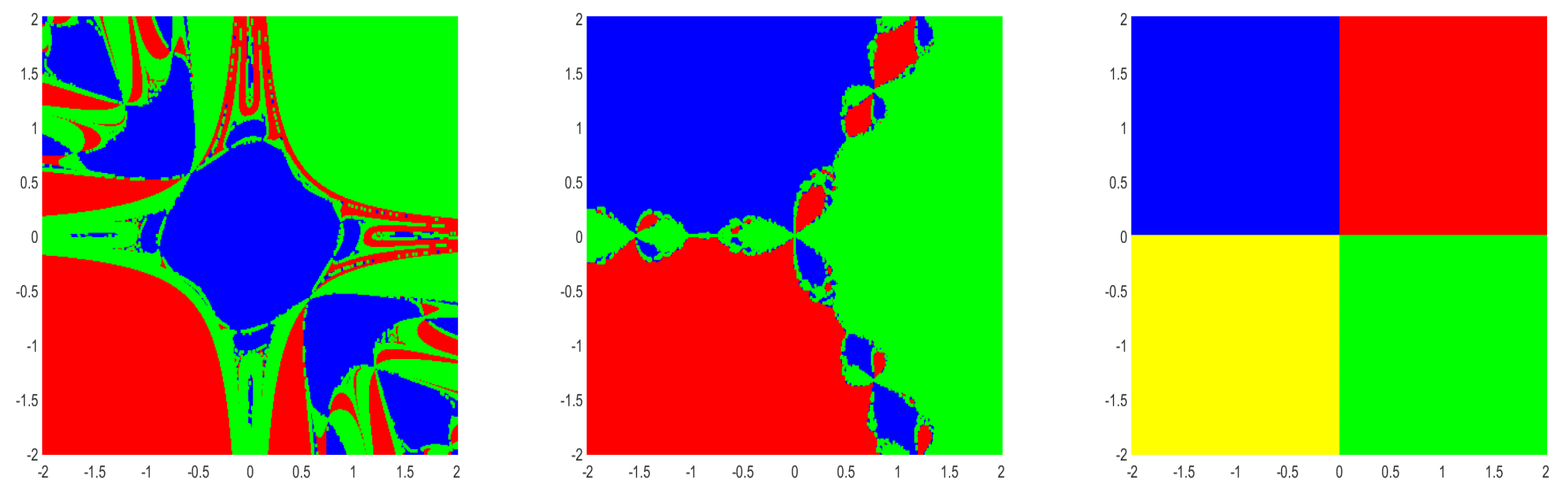
Figure 2.
Dynamical plane of the method (3) with Basins of attraction for Example 4(left), Example 5(middle) and Example 6(right).
Figure 2.
Dynamical plane of the method (3) with Basins of attraction for Example 4(left), Example 5(middle) and Example 6(right).
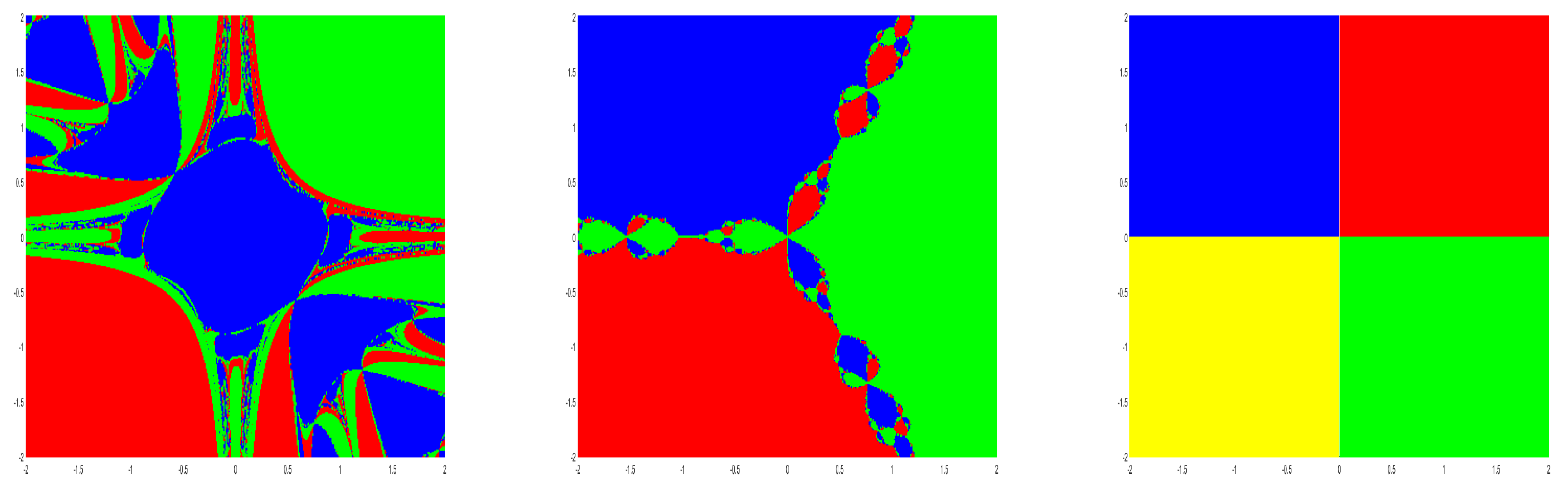
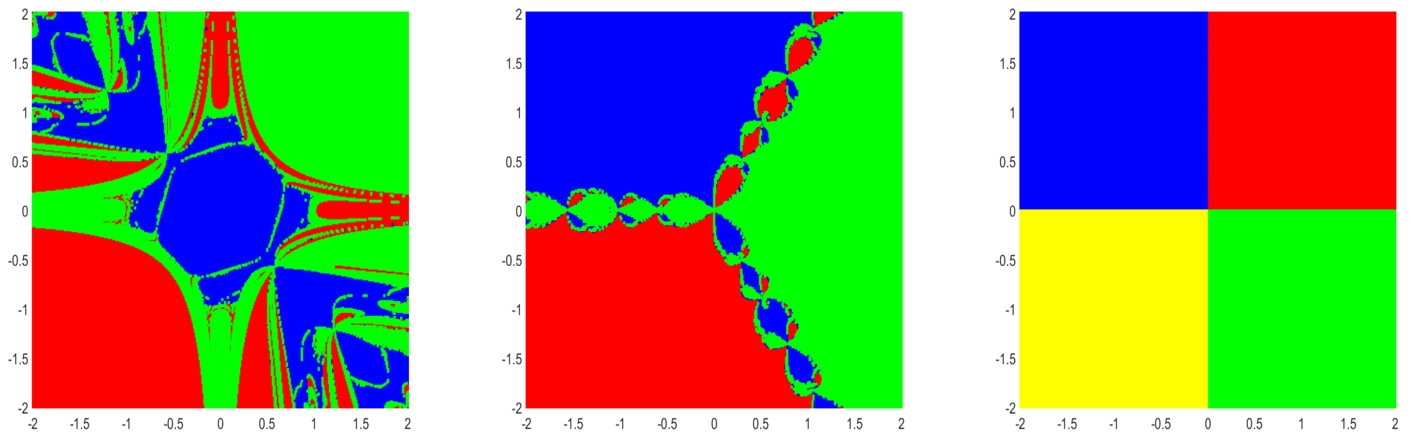
Figure 3.
Dynamical plane of the method (4) with Basins of attraction for Example 4(left), Example 5(middle) and Example 6(right).
Figure 3.
Dynamical plane of the method (4) with Basins of attraction for Example 4(left), Example 5(middle) and Example 6(right).
9. Conclusion
We studied Jarrat-type method of convergence order three and its two extensions with convergence order six and five, respectively. As mentioned in the introduction, we used assumptions on and only, so these methods (2), (3) and (4) can be used to solve problems which were not possible if we use the earlier convergence analysis using Taylor expansion. We discussed the limitations of our approach and developed new ways to overcome these limitations in Section 5. Finally, we compare the methods with other similar methods using an example. Also using Basins of attraction approach the convergence areas of the methods (2), (3) and (4) are given. In future research our ideas shall be applied on other methods to obtain similar benefits analogously [1,2,3,4,5,6,7,8,10,11,12,13,14,15,16,17,18,19,20,21,22,23,24]
References
- Argyros, I.K. The theory and applications of iteration methods. CRC Press, Engineering Series, Taylor and Francis Group 2022, 2. [Google Scholar]
- Argyros, I.K.; George, S. Extended Convergence Of Jarratt Type Methods. Appl. Math. E-Notes 2021, 21, 89–96. [Google Scholar]
- Bartle, R. G . Newton’s method in Banach spaces. Proceedings of the American Mathematical Society 1955, 6, 827–831. [Google Scholar]
- Behl, R.; Cordero, A.; Motsa, S.S.; Torregrosa, J. R. On developing fourth-order optimal families of methods for multiple roots and their dynamics. Applied Mathematics and Computation 2015, 265, 520–532. [Google Scholar] [CrossRef]
- Ben-Israel, A. A Newton-Raphson method for the solution of systems of equations. Journal of Mathematical analysis and applications 1966, 15, 243–252. [Google Scholar] [CrossRef]
- Cárdenas, E.; Castro, R.; Sierra, W. A Newton-type midpoint method with high efficiency index. Journal of Mathematical Analysis and Applications 2020, 491, 124381. [Google Scholar] [CrossRef]
- Chun, C.; Lee, M.Y.B.; Neta, B.; Džunić, J. On optimal fourth-order iterative methods free from second derivative and their dynamics. Applied mathematics and computation 2012, 218, 6427–6438. [Google Scholar] [CrossRef]
- Scott, M.; Neta, B.; Chun, C. Basin attractors for various methods. Applied Mathematics and Computation 2011, 218, 2584–2599. [Google Scholar] [CrossRef]
- Cordero, A.; Hueso, J.L.; Martínez, E.; Torregrosa, J.R. A modified Newton-Jarratt’s composition. Numer. Algor. 2010, 55, 87–99. [Google Scholar] [CrossRef]
- George, S.; Sadananda, R.; Jidesh, P.; Argyros, I.K. On the Order of Convergence of Noor-Waseem Method. Mathematics 2022, 10, 4544. [Google Scholar] [CrossRef]
- George, S.; Kunnarath, A.; Sadananda, R.; Jidesh, P.; Argyros, I.K. Order of convergence, extensions of Newton-Simpson method for solving nonlinear equations and their dynamics. Fractal Fract 2023, 163. [Google Scholar] [CrossRef]
- Iliev, A.; Iliev, I. Numerical method with order t for solving system nonlinear equations. Collection of scientific works 2000, 30, 3–4. [Google Scholar]
- Jarratt, P. Some fourth order multipoint iterative methods for solving equations. Mathematics of Computation 1966, 20, 434–437. [Google Scholar] [CrossRef]
- Magreñán, A.A. Different anomalies in a Jarratt family of iterative root finding methods. Appl. Math. Comput. 2014, 233, 29–38. [Google Scholar]
- Ortega, J.M.; Rheinboldt, W.C. terative solution of nonlinear equations in several variables. Society for Industrial and Applied Mathematics 2000, 14. [Google Scholar]
- Ostrowski, A.M. Solution of Equations and Systems of Equations: Pure and Applied Mathematics, A Series of Monographs and Textbooks. Elsevier 2016, 9. [Google Scholar]
- Petković, M.S.; Neta, B.; Petković, L.D.; Džunić, J. Multipoint methods for solving nonlinear equations: A survey. Applied Mathematics and Computation 2014, 226, 635–660. [Google Scholar] [CrossRef]
- Ren, H.; Wu, Q.; Bi, W. New variants of Jarratt’s method with sixth-order convergence. Numerical Algorithms 2099, 52, 585–603. [Google Scholar] [CrossRef]
- Saheya, B.; Chen, G.Q.; Sui, Y.K.; Wu, C.Y. A new Newton-like method for solving nonlinear equations. SpringerPlus 2016, 5, 1–3. [Google Scholar] [CrossRef]
- Shakhno, S. M.; Iakymchuk, R. P.; Yarmola, H. P. Convergence analysis of a two step method for the nonlinear squares problem with decomposition of operator. J. Numer. Appl. Math. 2018, 128, 82–95. [Google Scholar]
- Shakhno, S. M.; Gnatyshyn, O. P. On an iterative algorithm of order 1.839. . . for solving nonlinear operator equations. Appl. Math. Appl. 2005, 161, 253–264. [Google Scholar]
- Traub, J.F. Iterative methods for the solution of equations. American Mathematical Society 1982, 312. [Google Scholar] [CrossRef]
- Weerakoon, S.; Fernando, T. A variant of Newton’s method with accelerated third-order convergence. Applied mathematics letters 2000, 8, 87–93. [Google Scholar] [CrossRef]
- Werner, W. Über ein Verfahren der Ordnung 1+2 zur Nullstellenbestimmung. Numerische Mathematik 1979, 32, 333–342. [Google Scholar] [CrossRef]

Table 1.
Methods of order 3.
| k | Noor Waseem Method (67) | Ratio | Newton Simpson method (70) | Ratio | Method(3) | Ratio |
|---|---|---|---|---|---|---|
| 0 | (2.000000,-1.000000) | (2.000000,-1.000000) | (2.000000,-1.000000) | |||
| 1 | (1.264067,-0.166747) | 0.052791 | (1.263927,-0.166887) | 0.052792 | (1.151437,0.051449) | 0.040459 |
| 2 | (1.019624,0.265386) | 0.259247 | (1.019452,0.265424) | 0.259156 | (0.994771,0.304342) | 0.536597 |
| 3 | (0.992854,0.306346) | 1.578713 | (0.992853,0.306348) | 1.580144 | (0.992780,0.306440) | 1.951273 |
| 4 | (0.992780,0.306440) | 1.977941 | (0.992780,0.306440) | 1.977957 | (0.992780,0.306440) | 1.979028 |
| 5 | (0.992780,0.306440) | 1.979028 | (0.992780,0.306440) | 1.979028 | (0.992780,0.306440) | 1.979028 |
Table 2.
Methods of order 5.
| k | Noor Waseem Method (68) | Ratio | Newton Simpson method (71) | Ratio | Method(4) | Ratio |
|---|---|---|---|---|---|---|
| 0 | (2.000000,-1.000000) | (2.000000,-1.000000) | (2.000000,-1.000000) | |||
| 1 | (1.127204,0.054887) | 0.004363 | (1.127146,0.054883) | 0.004363 | (1.144528,0.069067) | 0.004375 |
| 2 | (0.993331,0.305731) | 0.501551 | (0.993328,0.305734) | 0.501670 | (0.994305,0.304922) | 0.495553 |
| 3 | (0.992780,0.306440) | 3.889725 | (0.992780,0.306440) | 3.889832 | (0.992780,0.306440) | 3.847630 |
| 4 | (0.992780,0.306440) | 3.916553 | (0.992780,0.306440) | 3.916553 | (0.992780,0.306440) | 3.916553 |
Table 3.
Methods of order 6.
| k | Noor Waseem Method (69) | Ratio | Newton Simpson method (72) | Ratio | Method(2) | Ratio |
|---|---|---|---|---|---|---|
| 0 | (2.000000,-1.000000) | (2.000000,-1.000000) | (2.000000,-1.000000) | |||
| 1 | (1.067979,0.174843) | 0.001211 | (1.067906,0.174885) | 0.001211 | (1.027012,0.256566) | 0.001057 |
| 2 | (0.992784,0.306436) | 1.383068 | (0.992784,0.306436) | 1.384152 | (0.992780,0.306440) | 3.122403 |
| 3 | (0.992780,0.306440) | 5.509412 | (0.992780,0.306440) | 5.509414 | (0.992780,0.306440) | 5.509727 |
Disclaimer/Publisher’s Note: The statements, opinions and data contained in all publications are solely those of the individual author(s) and contributor(s) and not of MDPI and/or the editor(s). MDPI and/or the editor(s) disclaim responsibility for any injury to people or property resulting from any ideas, methods, instructions or products referred to in the content. |
© 2025 by the authors. Licensee MDPI, Basel, Switzerland. This article is an open access article distributed under the terms and conditions of the Creative Commons Attribution (CC BY) license (http://creativecommons.org/licenses/by/4.0/).
Copyright: This open access article is published under a Creative Commons CC BY 4.0 license, which permit the free download, distribution, and reuse, provided that the author and preprint are cited in any reuse.


