Submitted:
10 April 2025
Posted:
14 April 2025
You are already at the latest version
Abstract
The stochastic processes [HMP (Homogeneous Markov), NHMP (Non‐Homogeneous Markov), SMP (Semi‐Markov), RP (Renewal), A&RP (Age and Repair)] used for reliability analyses (to the author knowledge) are particular cases of the G‐Process. We present the basics of RIT (Reliability Integral Theory) a theory able to deal with the G‐processes. It can be applied to Reliability, Availability, Maintenance and Statistical applications (Control Charts and Time Between Events Control Charts); its power allows the readers to prove that the T Charts and the reliability computations for repairable systems (e.g. the Duane method), used in Minitab 21 are wrong: various cases are considered, from published papers. due to lack of knowledge of RIT); moreover, with RIT anybody can prove that the T Charts and the reliability computations for repairable systems (e.g. the Duane method), used in Minitab 21 are wrong. We introduce the Stochastic G‐Processes, via the Integral Equations, which rule the relationships between the reliabilities Ri(t|s) related to the system states. We show the advantages of using RIT for Quality decisions (economics and business).
Keywords:
reliability integral theory
; G‐processes
; exponential distribution
; T charts
; minitab
; JMP
; costs by wrong ideas
1. Introduction
In 1999 the author met managers of a
"certified" company developing a new engine; he saw them using the
"Duane Method" for predicting the in-service MTBF by elaborating the
test reliability data. In 2022-23 he read various papers about Control Charts
with wrong Control Limits. Between 1999 and 2023, the author read a lot of
papers, of documents of Masters in RAMS (Reliability, Availability,
Maintenance, Safety) and books on quality, reliability, fatigue tests,
maintainability, maintenance, statistical tests for decision, Control charts,
Six Sigma, Taguchi methods, …, and unfortunately, he found many doubtful ideas
on the basics of Quality, Probability and Statistics (QPS).
Due to that, he decided to show his views about
such points.
These subjects can be dealt by Stochastic
Processes: there are several documents about them; a sample is in the
references [1,2,3,4,5,6]. Quality Methods, applied in
industries, depends on Stochastic Processes, information provided [7] and on Probability and Statistics [8–16]. Their knowledge is fundamental for taking
sound decisions: we will see the many wrong decisions taken by lack of
knowledge.
Since we consider Engineering Applications of
Stochastic Processes applied to physical systems in relation to the analysis of
their Quality and Reliability/Availability and state of Control, we model the
systems, by an engineering point of view, with a finite number of states
(finite state space) and continuous time.
We begin [17–23]
by presenting it here through a quite simple example, a stand-by repairable
system of two units, A and B, with reliabilities RA(t) and RB(t)
for the “mission time” (interval) 0-----t. The system can be
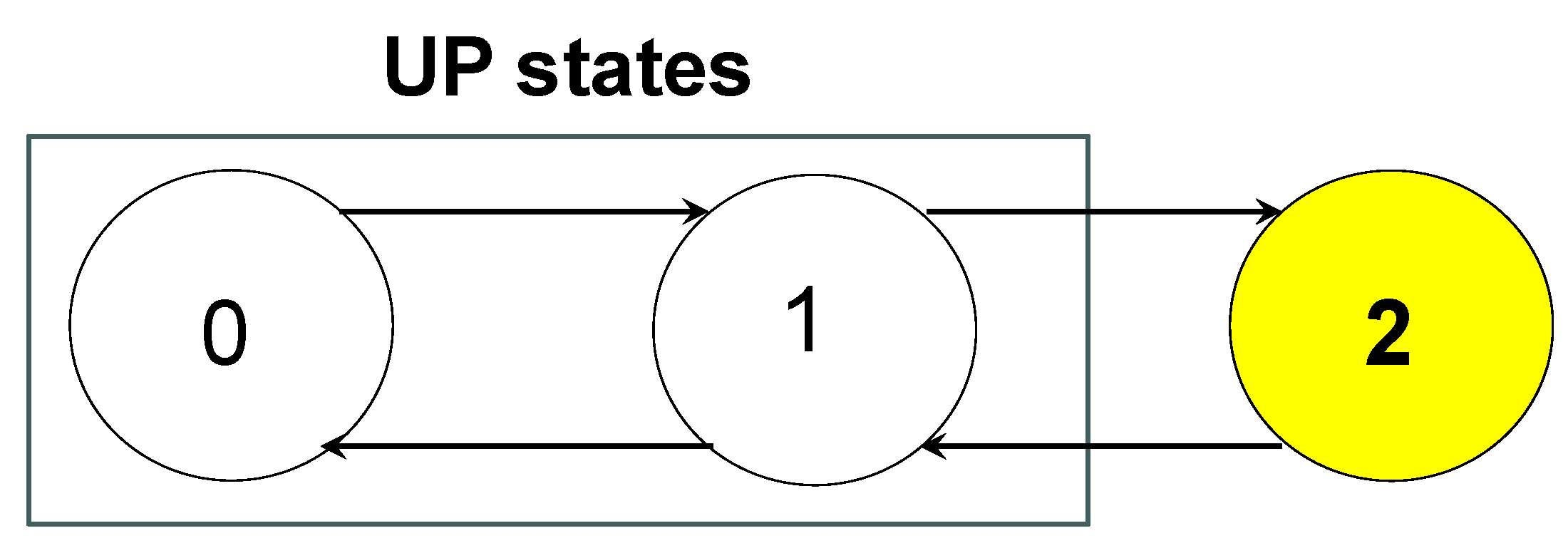
depicted as a three-state (Figure 1)
process (representing the system with states 0 (unit A is working and B is in
stand-by), 1 (unit A fails at some instant s<t and B starts working), 2
(both units are failed). The state space is denoted by S={0, 1, 2};
it is partitioned into disjoint sets S1={0, 1}, the set of the
Up-states and S2={2}, the set of the Down-states (only one in
the Figure 1, yellow coloured). Forward
transitions are related to failures of the units while backward transitions are
related to repair of the units; the system fails if it enters the set S2;
any transition from S2 to S1 restores the system to a
working condition; we did not depict the “inner transitions” j→j, showing that the system remains in the
same state j. The system is reliable as soon it makes transitions within S1:
for each Up-state j ∈ S1 we
define a reliability function Rj(t) which is the probability that the
system does not fail (i.e. does not enter the set S2), for the
“mission time” (interval) 0-----t, while for each state j ∈ S we define an availability function Aj(t)
which is the probability that the system is not failed (i.e. does not enter the
set S2), at the instant t.
Figure 1.
Transitions of a Stochastic Process.
For a single unit we define the "failure
rate" h(t)=f(t)/R(t) which generally depends on t. IF and only IF h(t)=,
a constant not depending on t, then MTTF=1/, and =1/MTTF
and R(t)=exp(-t): exponential reliability, the item is always "as good as
new". In any other case the failure rate is h(t)1/MTTF,
and hence MTTF1/h(t). For the Weibull distribution (
characteristic life, shape parameter) R(t)=exp[-(t/)],
the failure rate h(t)=(/)(t/)-1, and hence MTTF1/h(t):
many professionals do not know that [17–23].
Consider what we found on an EJTAS paper December
2023 “A New Approach for Effective Reliability Management of Biomedical
Equipment” (3 Indian authors): there “Reliability is defined as the
probability that an equipment or process performs its intended function
adequately for a specified period of in a defined environment
without failure.” What is wrong with the definition? The specified period
is not the interval 0----t. They add, later, “where ′μ′ is mean of time
between failure (MTBF), ′σ′ is standard deviation of MTBF and ′x′ is breakdown
time”. This is misleading because they confuse MTBF with MTTF [a
constant value equal to the area below R(t)] and confuse the “standard
deviation of the RV T” with the standard deviation of MTBF. We
will see some their other problems later. They are in good company… See the
Excerpt 1.
To be more general we define the interval
reliability R(t|r) as the probability that the system does not fail in the
interval r----t, given that it did not fail before r.
For reliability analysis we have to consider (in Figure 1) R0(t|r) and R1(t|r)
where r is the instant of entrance into the states 0 and 1, respectively.
Excerpt 1.
Some documents with several drawbacks.
For availability analysis we have to consider (in Figure 1) A0(t|r), A1(t|r)
and A2(t|r) where r is the instant of entrance into the states 0, 1
and 2, respectively: Aj(t|r) is the probability that the system is
not failed at the instant t.
The functions Rj(t|r) and Aj(t|r)
depend on the probabilities of the various transitions (failures or repair of
the units).
Letting S(t) the state occupied by the system at
time t, we have that S(t), at time t, is a Random Variable taking the values in
the state space S=S1∪S2={0, 1, …, nU, nU+1, …,
N}: N+1 is the number of states. The
(“real”) variable t is a parameter indexing the Stochastic Process S(t).
Safety, Reliability, Maintainability, Conformity,
Durability, Service, Process Control, Testing, are some of the most important
dimensions of Quality; they must be taken into account during Product
Development. To make Quality of products and services, knowledge of Quality
ideas and Quality tools for achieving Quality are absolutely needed, for any
person involved in any Company management (Universities, as well …). To find
and use the Quality tools for Quality achievement, education of Managers on
Quality is essential. Unfortunately, too many managers [and not only managers
...] do not know much about Quality ideas and Methods; see Deming statements
(in his exceptionally good books) [24,25]:
Excerpt 2.
Some statements of Deming about Knowledge and Theory (Deming 1986, 1997).
In the author's opinion, the first step to Quality
achievement, through problem prevention, is to define logically
what Quality is. It is very important defining correctly what Quality means,
because Quality is a serious and difficult business; to provide a practical and
managerial definition, since 1985 F. Galetto was proposing the following one: Quality
is the set of characteristics of a system that makes it able to satisfy the NEEDS of the Customer, of the User and
of the Society. This definition highlights the importance of the needs
of the three actors: the Customer, the User and the Society. Prevention
is the fundamental idea present in this definition: you possibly satisfy
the needs only by preventing the occurrence of any problem against the
needs.
To measure and analyse the «Characteristics»
of Quality during the total life of a product, from its design until its use in
the field we NEED Probability Theory [1–30]:
for this reason, we decided to write this paper on the Stochastic Processes.
2. Materials and Methods
2.1. Reliability Integral Theory (RIT)
Let’s now show how RIT manages the (Stochastic
Processes) for reliability analysis of physical systems.
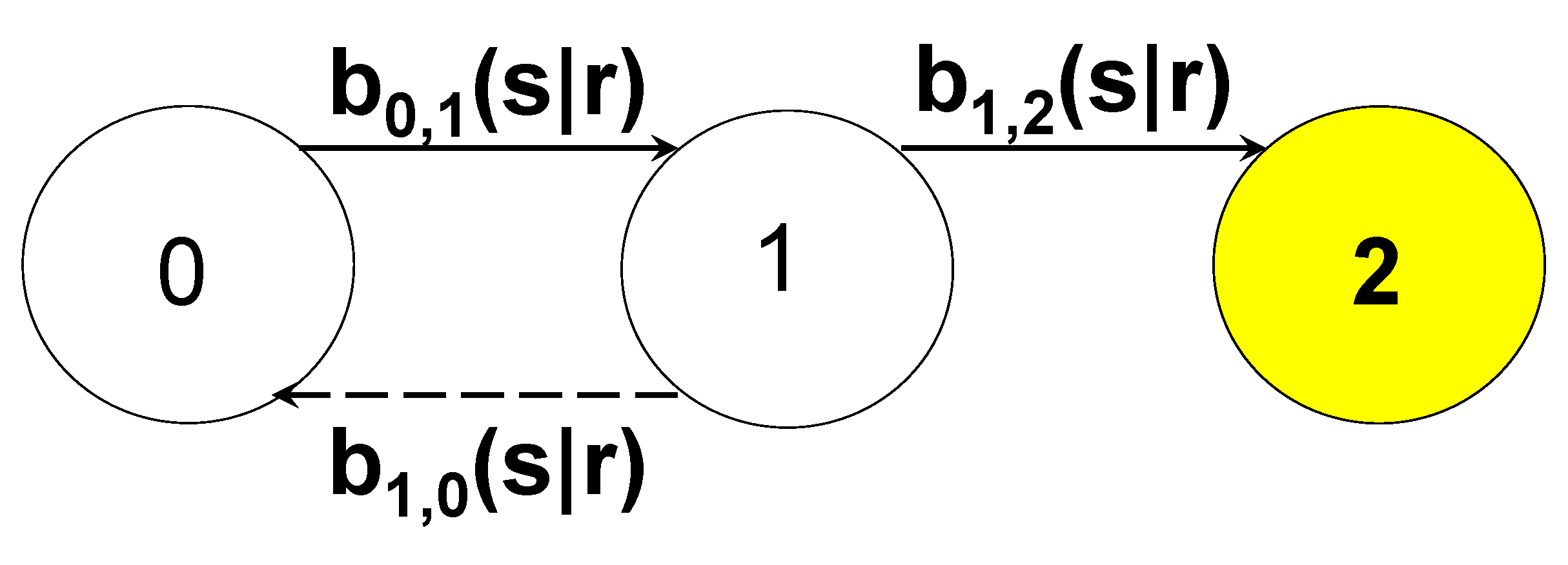
We use the Figure 2
(it is like the Figure 1, without the
transition 2→1): if the system fails,
enters the state 2, it remains there forever. In the model the transitions are
ruled by some functions bi,j(s|r) named kernels, related to
the interval reliability Runit(t|r) of the units and by the
probability of repair of the failed units.
The instant “r” is the time of entrance into a
state, while “s” is the time instant of leaving a state.
Rj(t|r) [reliability associated to
the state j] is the probability that the system is working, at time t, i.e.
[S(t)=j]∈S1={0, 1, …, nU}, when it entered the state j at time r of
the “mission time”, r∈0----t.
The functions bi,j(s|r)ds are the instantaneous probability
of transition from state i to state j and are the probabilities of staying in the state i
for the whole interval r----t.
Figure 2.
Transitions of a Reliability Stochastic Process.
Applying the probability theory, we can write the
two general equations (1) [related to the model in Figure 2]
The two equations (1) are Integral Equations
with unknown functions Rj(t|r); we name the previous equations the fundamental
system of the Reliability Integral Theory (RIT).
We name G-Processes the stochastic
processes ruled by the Integral Equations (1).
For any type of system, we write
where is the column vector of the reliabilities Rj(t|r),
j∈S1={0, 1, …, nU},
is the kernel matrix and , j∈S1={0, 1, …, nU}, is the diagonal matrix of the waiting
functions in the up-states before any transition.
It is the fundamental system of the Reliability
Integral Theory.
The unknown reliabilities Rj(t|r)
depends on the kernels bi,j(s|r), related to the failure rate
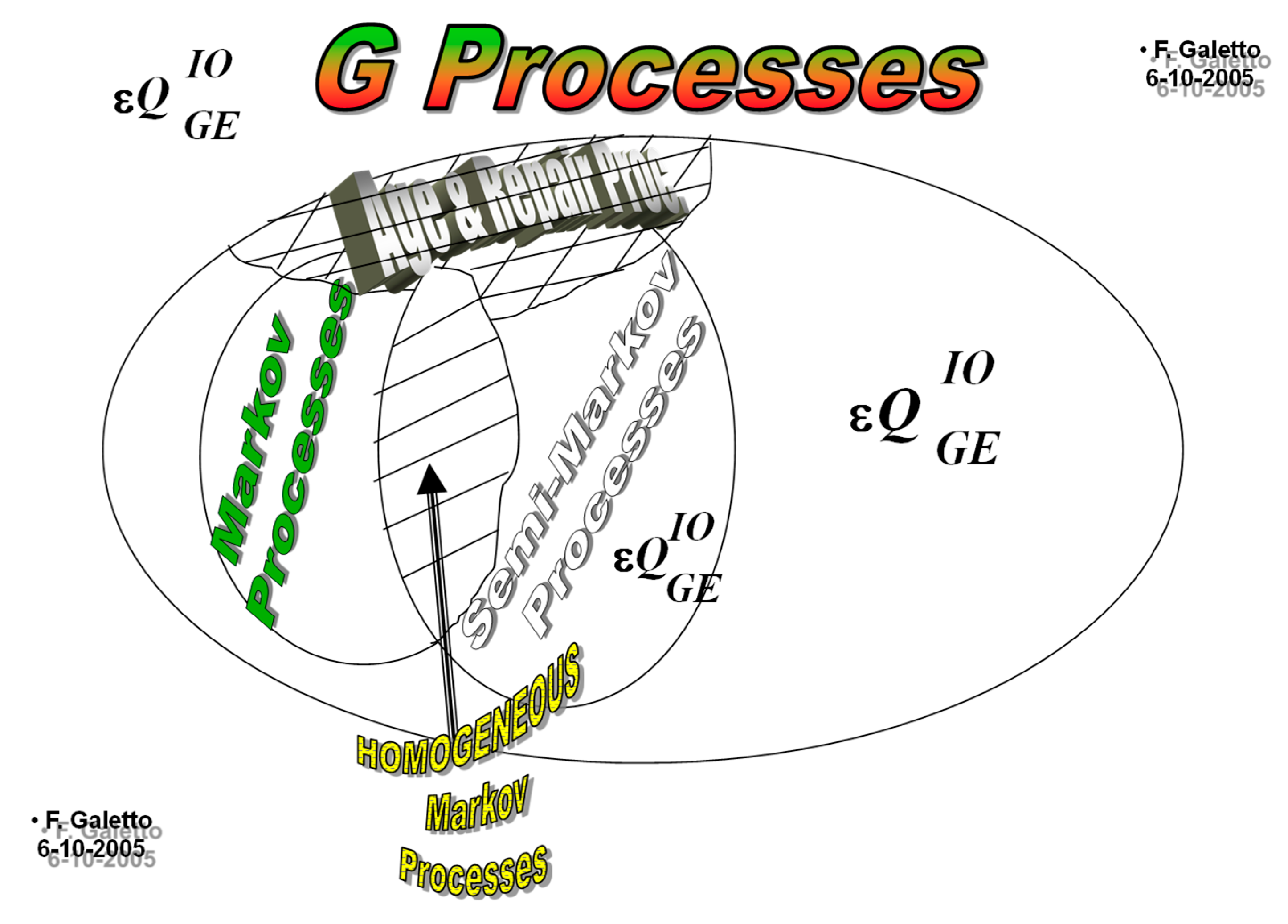
and the repair rate of the units; if they assume some particular form then the G-Processes
become known processes [1–6] (see Figure 3): Homogeneous Markov Processes (HMP),
Non-Homogeneous Markov Processes (NHMP), Semi-Markov Processes (SMP), Poisson
Processes (PP), Wiener Processes (WP), Branching Processes (BP), Birth and
Death Processes (BDP), …
Figure 3.
G-Processes comprise several Stochastic Processes (depending on the kernels).
To the author knowledge, there is no Theory (but
RIT) able to deal the Age& Repair (A&R) processes, where the forward
transitions depend on the age of the system, i.e. bi,j(s|r)=bi,j(s),
and the repair (backward transitions) depend on the time interval r-----s
from the entrance r into a state, i.e. bi,j(s|r)=bi,j(s-r).
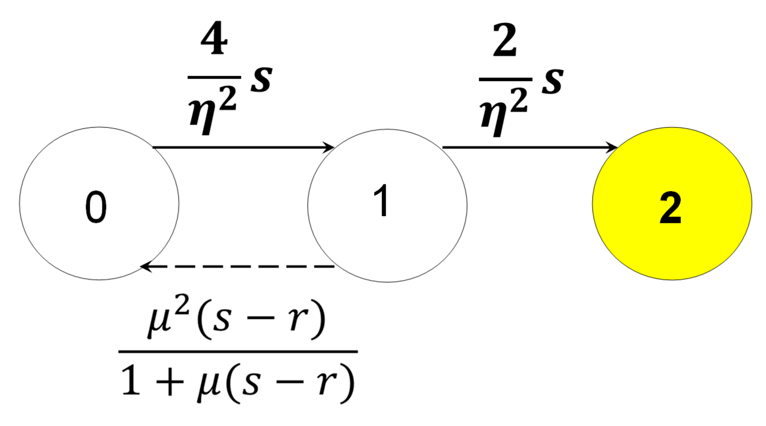
The transition rates are as in the Figure 4
(an example of a “parallel system of 2 identical units” with Weibull
reliability and Erlang repair of the failed unit)
Figure 4.
Transitions of an Age & Repair Stochastic Process (transition rates).
Generally, we are interested to the interval 0-----t
(mission time) and then we compute the two functions R0(t)=R0(t|0)
and R1(t)=R1(t|0).
If both the kernels are exponential (no aging
behaviour) we can draw a flow graph with the transition rates λ (failure rate) and μ (repair rate) and write the matrix equation where R(t) is the
column vector with entries R0(t) and R1(t) and A the
“transition” matrix (see Figure 4 for the
parallel, where there is no age)
(3) is the model of a Homogeneous Markov Processes
(HMP).
For a renewable system we write
It is the fundamental system of the Reliability
Integral Theory, for SEMI-Markov processes (SMP).
From the reliabilities we compute the two Mean Time
To (system) Failure MTTF0 and MTTF1: (MTTF not MTBF…)
For HMP and SP we can get the MTTFs without
actually computing R0(t) and R1(t), as follows
where m0 and m1 are the mean
holding time in the up-states 0 and 1, and p0,1 and p1,0
are the steady state transition probabilities from 0 to 1 and from 1 to 0.
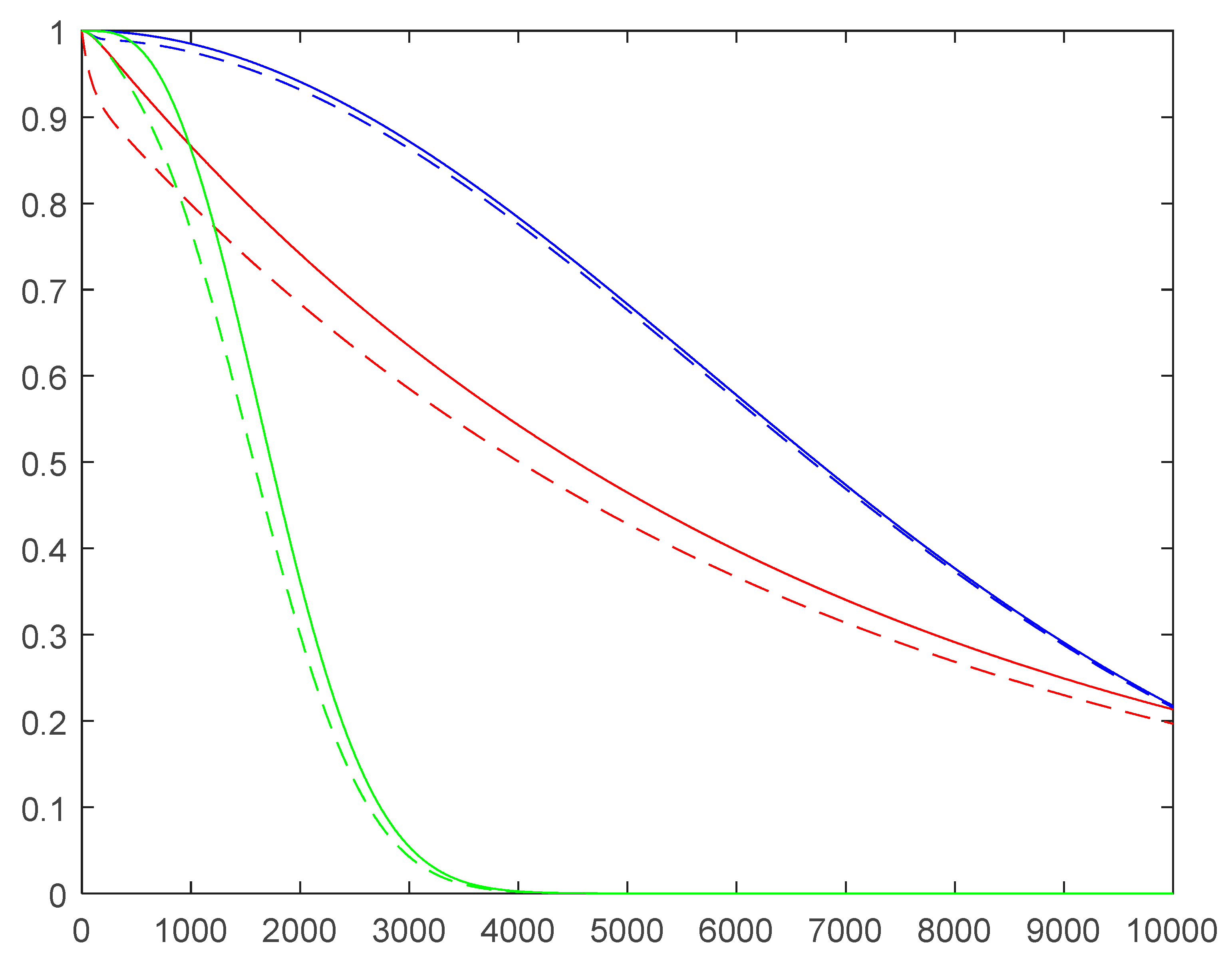
It is very useful (Figure
5) to see the difference of the various reliabilities R0(t)
and R1(t) dealt with the three stochastic processes: Homogeneous
(red curves), Non-Homogeneous (blue curves), Age&Repair (green curves).
Notice that the reliabilities
generated by the NHMP (with linear failure and repair rates) are
the highest curves; that does not mean that they are the best curves: the
linear repair rate is such that it depends on the age of the system (the
older the system, the higher the repair rate: absurd!): this
causes huge costs, due to wrong analyses and decisions.
Figure 5.
R0(t) and R1(t) for the HMP (red curves), for the NHMP (blue curves) and for the A&RP (green curves).
Figure 5.
R0(t) and R1(t) for the HMP (red curves), for the NHMP (blue curves) and for the A&RP (green curves).
It is clear that when the failure rate is
increasing (due to wear out) we can benefit from “Preventive Maintenance”: the
units are replaced before they fail. Optimized Maintenance Actions (based on
reliability, costs of repairs and cost of Preventive Maintenance, and Spare
parts Availability) improve the earning of Systems.
To do that we need suitable Methods.
By integrating from 0 to ∞ the column vector in the formula (4) we find the column vector of
the system MTTFj, j∈S1={0, 1, …, nU},
where P is the matrix of the steady transition probabilities between the Up-states and M the diagonal matrix of the “Mean Holding Time mj“ (the length of time in the state j, before transition).
So, we see that we can compute the MTTF, without actually computing the column vector ; we need only M and P
The matrix provides the “Mean Number of Transitions Between the Up-states, before the system failure”.
Notice that we can use the formula (7) only for the Semi-Markov Processes; hence in the Figure 5 we must compute by numerical methods the area below the blue and green curves.
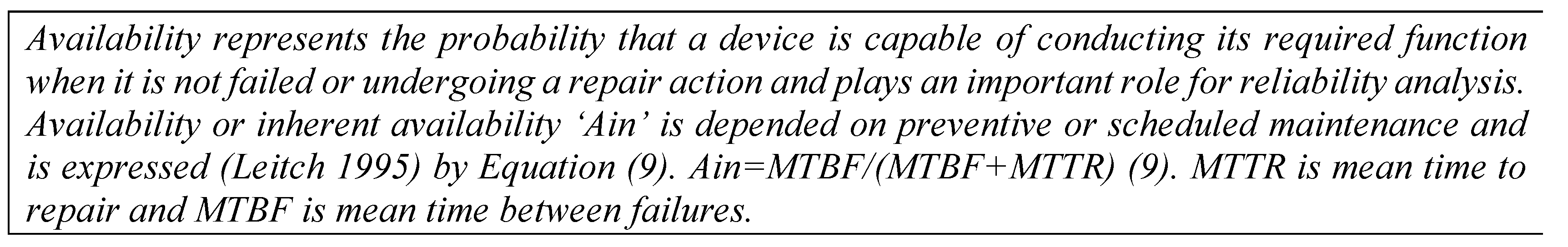
2.2. Availability Integral Theory (AIT)
If we (Figure 1) allow that the failed system, in the state 2, be repaired [transition from 2 to 1, with kernel b2,1(s|r)] we can study the system Availability associated to the states S={0, 1, 2}, A0(t|r), A1(t|r), A2(t|r); S is divided into two disjoint sets S=S1(up states {0, 1})∪ S2(down states {2}); Ai(t|r) [availability associated to state i], [S(t)=i]∈S={0, 1, …, nU, nU +1, N}, is the probability that the system is working [in the up states, S1], when it entered the state i∈S at time r. Following the same lines, we can write the following fundamental system of the Availability Integral Theory, AIT) [holding whichever is the distributions of the time to failures and times to repair of the various units]; the stochastic process ruling the transitions is named G-Process: all the quantities are computed using the kernels bi,j(s|r).
When t→∞ all the availabilities A0(t), A1(t), A2(t) approach the same value ASS=MUT/MTBF =MUT/(MUT+MDT), the steady state Availability (proved in the author’s books).
Notice the differences with the EJTAS paper December 2023 “A New Approach… of Biomedical Equipment” where we find (…, excerpt 3)
Same problems are found in the Excerpt 1.
For a general SMP we can derive that
ASS=MUT/MTBF =MUT/(MUT+MDT) (9)
where MUT is the Mean Up Time, a suitable mean of the MTTFi, from i∈S1={0, 1, …, nU} to S2={nU+1,…, N} in the steady state, and MDT is the Mean Down Time, a suitable mean of the MTTRj, from j∈ S2={nU+1,…, N} to S1={0, 1, …, nU} in the steady state [17,18,19,20,21,22,23].
Excerpt 3.
From “A New Approach…”.
2.3. Statistics and RIT
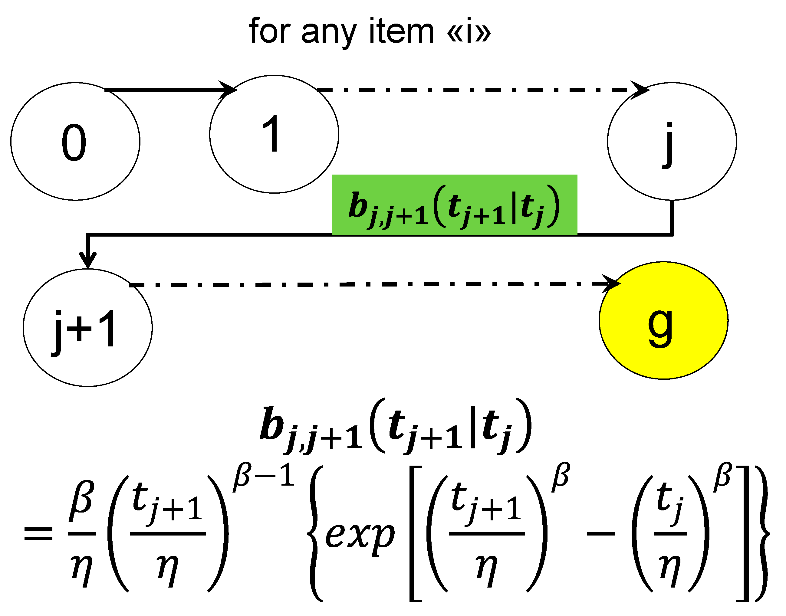
RIT (G-Processes) can be used for parameters estimation and Confidence Intervals (CI), (Galetto 1981, 1982, 1995, 2010, 2015, 2016), in particular for Control Charts (Deming, 1986, 1997, Shewhart 1931, 1936, Galetto 2004, 2006, 2015). In fact, any Statistical (or Reliability) Test can be depicted by an “Associated Stand-by System” whose transitions are ruled by the kernels bk,j(s); we can write the fundamental system of integral equations for the reliability tests, whose duration t is related to interval 0-----t; the collected data tj can be viewed as the times of the various failures (of the units comprising the System) [t0=0 is the start of the test, t is the end of the test and g is the number of the data]
is the probability that the stand-by system (statistical test or CC) does not enter the state g, at time t, when it starts in the state j at time tj, is the probability that the system does not leave the state j, is the probability that the system makes the transition j → j+1.
The reliability system (10) can be written in matrix form,
At the end of the reliability test, at time t, we know the data (the times of the transitions tj) and the empirical sampleD={x1, x2, …, xg}, with xj=tj – tj-1 is the length between the transitions; the transition instants are tj = tj-1 + xj giving D*={t1, t2, …, tg-1, tg, t}; t is the duration of the test.
We consider now that we want to estimate the unknown MTTF=θ=1/λ of each item comprising the stand-by system: each datum is a measurement from the exponential pdf; we compute the determinant of the integral system (11), where is the “Total Time on Test” . At the end time t, the integral equations, constrained by the constraintD*, provide the equation
In the case of exponential distribution, it is exactly the same result as the one provided by the MLM Maximum Likelihood Method [1,2,3,4,5,6,7,8,9,10,11,12,13,14,15,16].
If the data are normally distributed, , with sample size n, then we get the usual estimator such that .
The same happens with any other distribution provided that we can write the kernel .
The reliability function , [formula (10)], with the parameter , of the “Associated Stand-by System” provides the Operating Characteristic Curve (OC Curve, reliability of the system) [8,9,10,11,12,13,14,15,16,17,18,19,20,21,22,23,30,35] and allows to find the Confidence Limits ( Lower and Upper) of the “unknown” mean , to be estimated, for any type of distribution (Exponential, Weibull, Rayleigh, Normal, Gamma, …); by solving, with unknown , the two equations (|) we get the two values (, ) such that
where is the “total of the length of the transitions xi=tj - tj-1 data of the empirical sample D” and CL= is the Confidence Level. CI=-------- is the Confidence Interval of .
The same procedure can be used for normal data as those of the paper “The mixed CUSUM-EWMA (MCE) Control Chart as a new alternative in the Monitoring of a Manufacturing Process” published in the Brazilian Journal of Operations & Production Management, pp. 1-13, DOI: 10.14488/BJOPM.2019.v16.n1.a1, written by 6 authors.
Consider the 30 data and the authors’ Control Chart
| 69.80 | 69.50 | 68.80 | 70.90 | 69.20 | 70.40 | 71.00 | 71.30 | 70.00 | 70.10 |
| 72.10 | 69.90 | 70.10 | 70.30 | 71.20 | 70.80 | 70.70 | 69.95 | 71.20 | 71.35 |
| 71.35 | 69.90 | 70.25 | 70.50 | 70.28 | 71.30 | 70.20 | 70.35 | 70.15 | 70.10 |
The 6 authors write: “The statistical analysis of this manufacturing process is obtained from 30 samples of size n=1. The first seven (7) samples of this process behaved according to a normal distribution with a mean of μ=70 equivalent to the nominal value and standard deviation σ=1. i.e., N (70,1), and the 23 remaining samples had a change of 0,5σ in the mean, or N (70.5,1).”
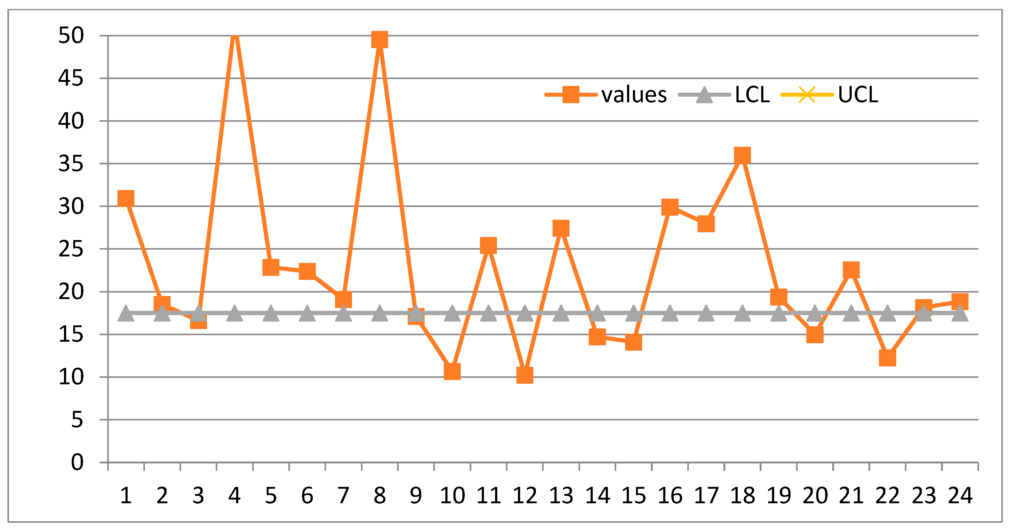
The authors wrongly stated that (verbatim): “… the EWMA (Figure 10, not reported here), CUSUM (Figure 11, not reported here) and Shewhart type (3σ) (Figure 12, given below as Figure 6) control charts cannot detect any situation out of control for the dataset provided.”
Notice: the process appears IC because in the Figure 6 the Control Limits do not depend on the collected data; actually, they are the Probability Limits of the Probability Interval.
7: the process is OOC! It is very clear that the Process is Out Of Control (OOC), due to two causes:
- a)
- Two points out of the Control Limits, and
- b)
- The points from 8 to 30 have a mean larger than the mean of the first seven points
Notice that the process is OOC in two ways: a) because one point is below LCL and one point is above UCL, b) because the mean of the last 23 points is statistically different form the mean of the first 7 points.
The Brazilian Journal … Management, did not publish the letter to the Editors.
2.4. Control Charts for Process Management
Statistical Process Management (SPM) entails statistical Theory and tools used for monitoring any type of a process, industrial or not. The Control Charts are the tool used for monitoring a process, to assess two states: the first, when the process, named IC (In Control), operates under the common causes of variation (variation is always naturally present) and second, named OOC (Out Of Control), when the process operates under some assignable causes of variation. The CCs, using the observed data, allow us to decide if the process is IC or OOC.
Control Charts were very considered by Deming (1986, 1997) and Juran (1988) after Shewhart invention (1931, 1936).
We start with Shewhart ideas (see the excerpt 4). He wrote on page 294, where is the “Grand Mean”, computed from D, is “estimated standard of each sample” (with sample size n), is the “estimated mean standard deviation of all the samples”.
Excerpt 4.
From Shewhart book (1931).

From Excerpt 4, we clearly see that Shewhart, the inventor of the CCs, used the “Normal Approximation (Central Limit Theorem)” [8,9,10,11,12,13,14,15,16] and the data to compute the Control Limits, LCL (Lower Control Limit) and UCL (Upper Control Limit) both for the mean (the 1st parameter of the Normal pdf) and for (the 2nd parameter of the Normal pdf). Similar ideas can be found in Dore, 1962, Belz, 1973, Ryan, 1989, Rao, 1965, Cramer, 1961, Mood, 1963, Rozanov, 1975 (where we see the idea that CCs can be viewed as a Stochastic Process). See also F. Galetto [19,30,35].
Compare Excerpt 4 (where LCL, UCL depend on the data) with Excerpt 5 (where LCL, UCL depend on the Random Variables) and appreciate the profound difference: this is the cause of the many errors in the CCs for TBE (Time Between Events (see the “Garden…” ). Notice that an author wrote several papers… Notice the wrong statement (with k=3) “The control limits of the standard Shewhart chart ( chart or the X chart) are given by UCL1=μY+3σY and LCL1=μY-3σY where μY and σY are the specified IC mean and standard deviation of the charting statistic Yi”. Notice that, as per Excerpt 5, L=μY-3σY------U=μY+3σY is not the CI (Confidence Interval) of the mean μ=μY (as in Excerpt 4) but the Probability Interval such that the RV Y
The same error is in other books (e.g. Montgomery D., 1996-2019, page 192-3). The right ideas are in Galetto F. (2006, 2015, 2016). RIT will show clearly the drawbacks of those many authors (Galetto 1981, 2006, 2015, 2016).
Excerpt 5.
From Control Charts, Synthetic (2021), a paper in the “Garden…”. Notice that one of the authors wrote several papers….
Excerpt 5.
From Control Charts, Synthetic (2021), a paper in the “Garden…”. Notice that one of the authors wrote several papers….
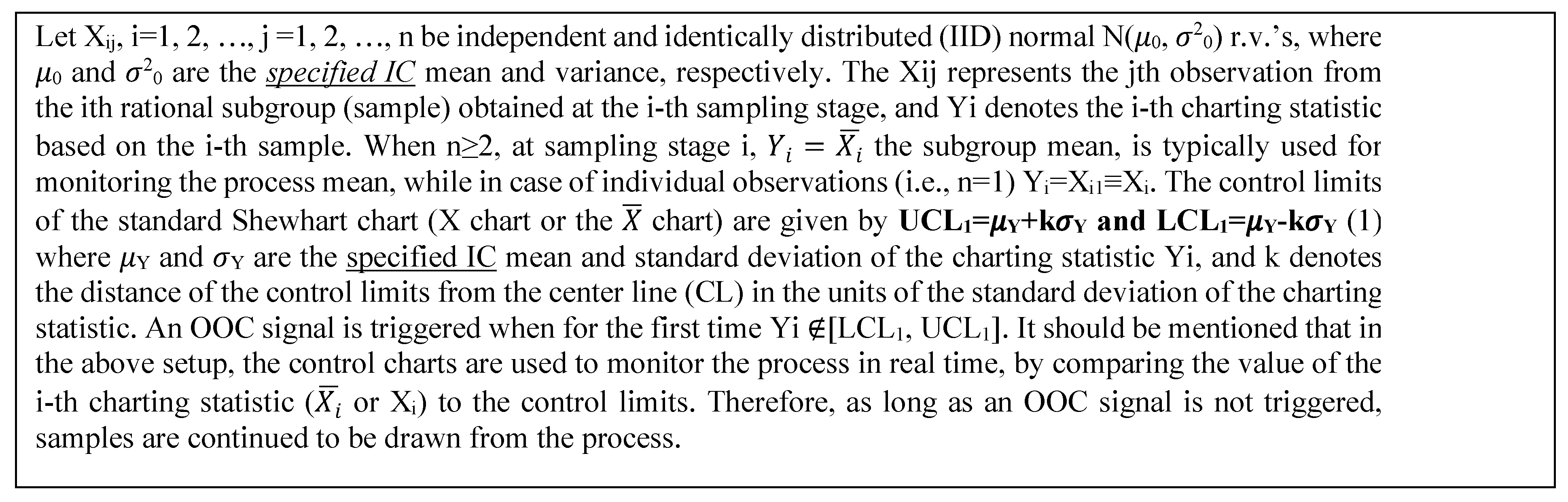
Notice, in the Excerpt 5, the statement “… in case of individual observations (i.e. n=1)… the Control Limits…”.
It is very interesting that a Peer Reviewer chosen by the Editors of Quality and Reliability Engineering International (QREI) suggested (February 2024) the author to read the following paper in order to learn the way to compute the Control Limits for Individual Control Charts with Exponentially distributed data:

We anticipate our conclusion about the Excerpt 6:
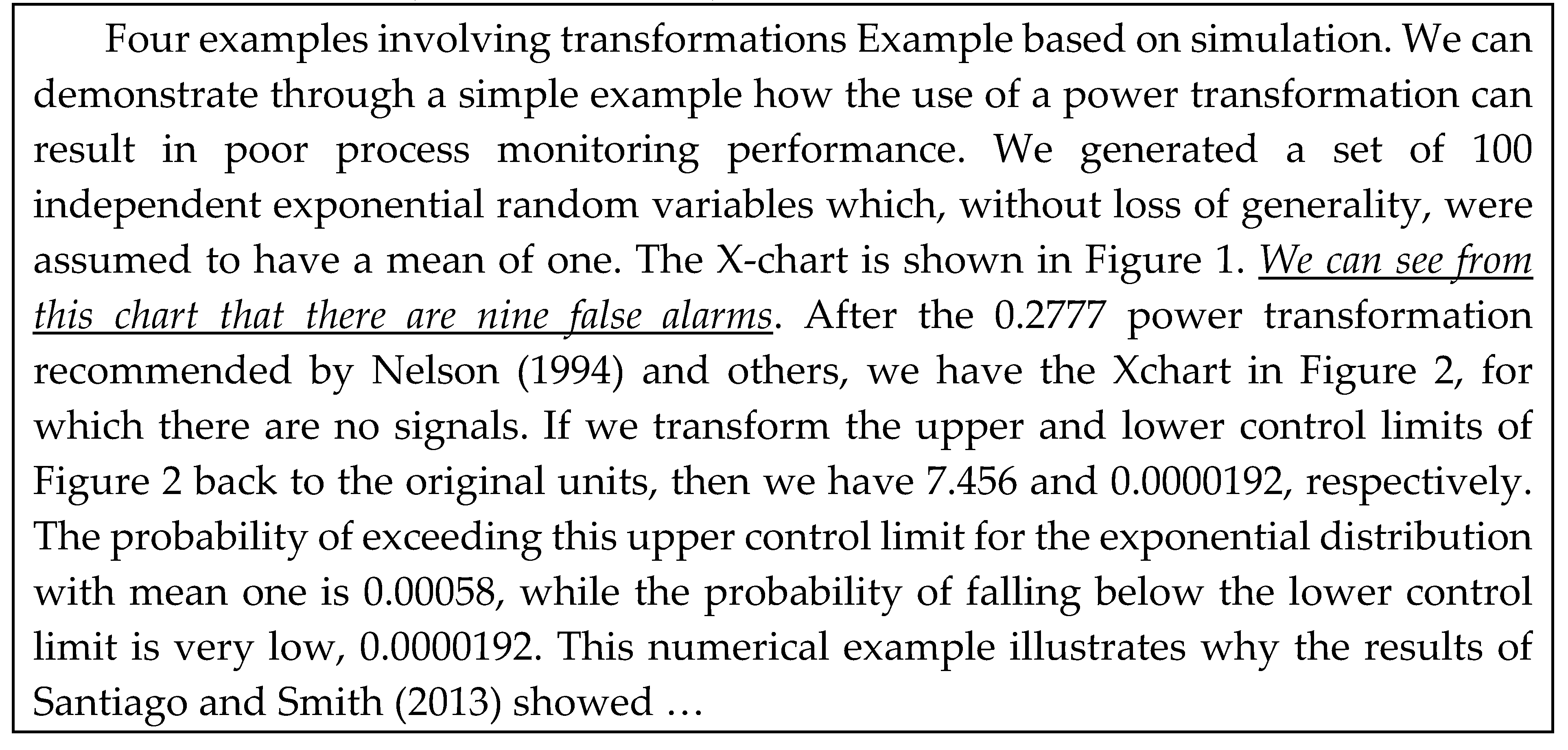
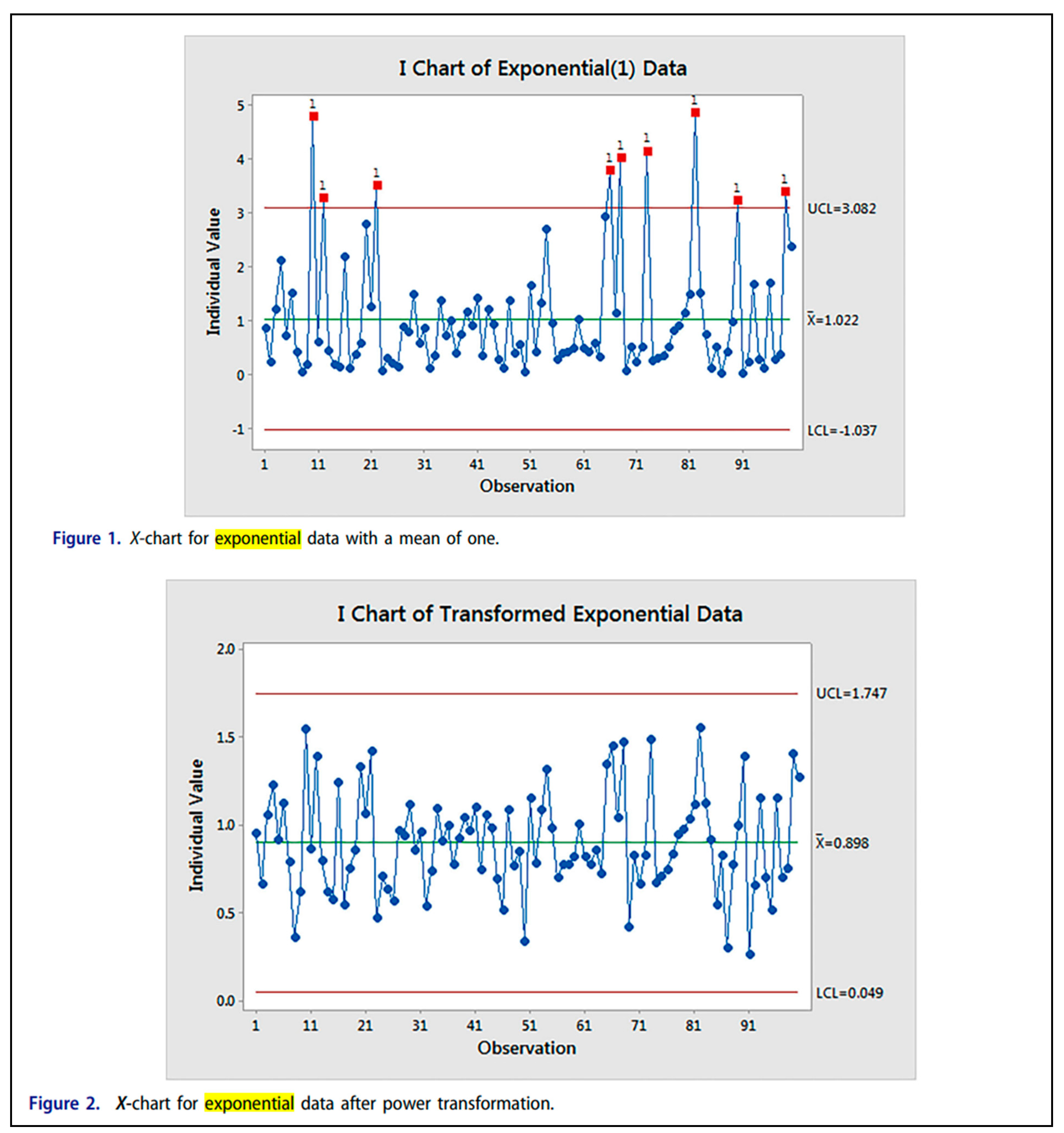
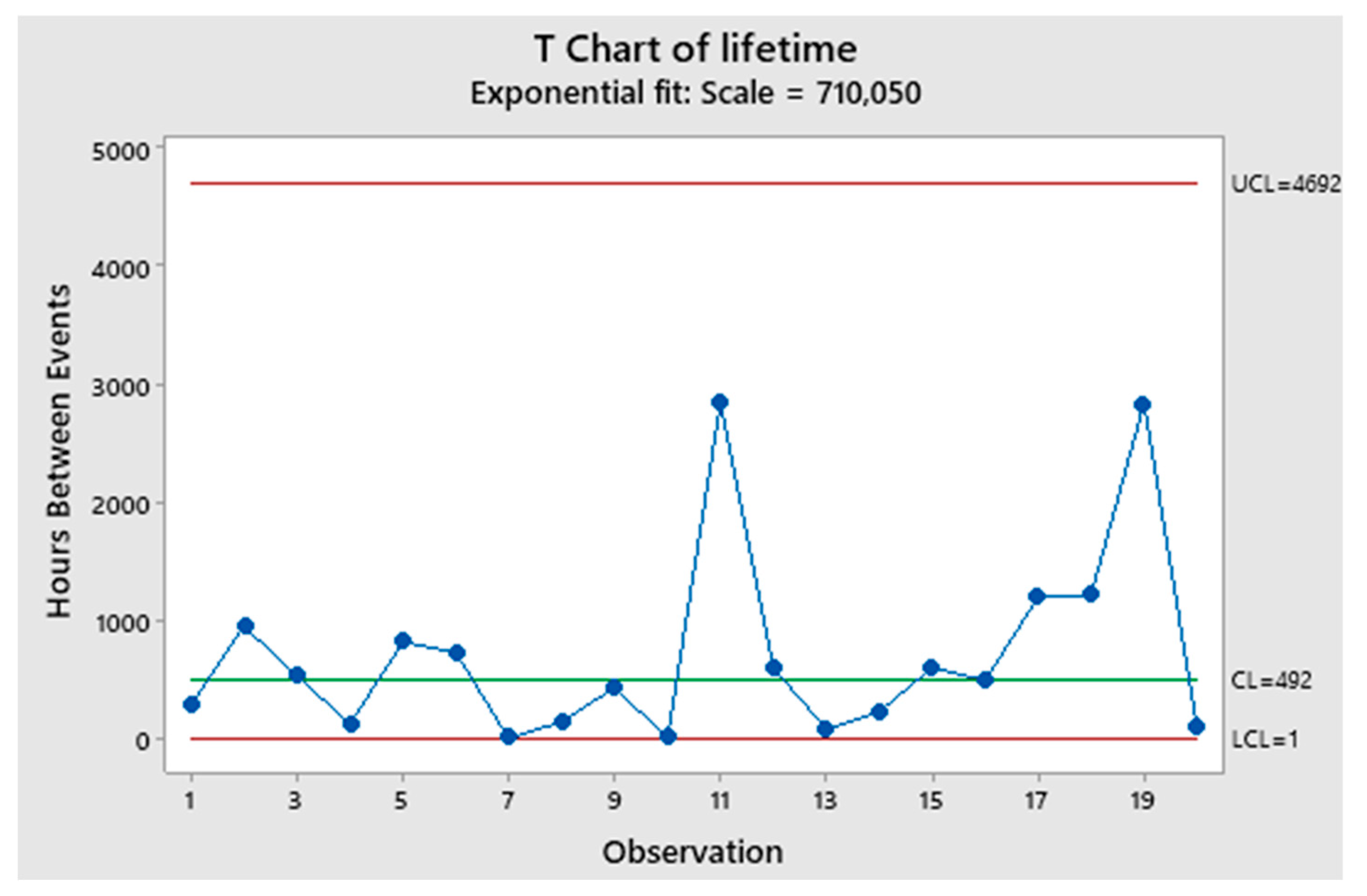
The 3 authors statement (in the Excerpt 6) “We can see from this chart that there are nine false alarms. (see the Figure 1, in the Excerpt 6)” IS WRONG.
LCL=0.103 and UCL>>100
From the Figure 1 we cannot read the value of the data, BUT surely there are NO … false alarms (above the TRUE UCL) (Figure 1, in the Excerpt 6).
IF we had the data, we could assess that there could be Out Of Control, BELOW the LCL…
The Peer Reviewer did not know the TRUE Theory, as did not the authors.
Notice the wrong LCL=1.022-2.06 and UCL=1.022+2.06 in the Figure 1 (in the Excerpt 6): they are computed with the wrong formula given in the Excerpt 5 (as though the Exponential data were Normal data!): Nonsense!
All the people involved did not know that also the differences |xi+1-xi| are exponentially distributed.
The 3 authors write (authors’ statements):
Excerpt 6.
From the paper The role of the normal distribution in statistical process monitoring.
Generally, the data plotted are the means , determinations of the Random Variables , i=1, 2, ..., n (n=number of the samples) computed from the collected data xij, j=1, 2, ..., k (k=sample size), determinations of the RVs at very close instants tij, j=1, 2, ..., k. In other applications, the data plotted are the Individual Data , determinations of the Individual Random Variables , i=1, 2, ..., n (n=number of the collected data), modelling the measurement process of the “Quality Characteristic” of the product: this model is very general because it is able to consider every distribution of the Stochastic Process .
Shewhart on page 289 of his book (1931) writes “… we saw that, no matter what the nature of the distribution function of the quality is, the distribution of the arithmetic mean approaches normality rapidly with increase in n (his n is our k, the sample size), and in all cases the expected value of means of samples of n (our k) is the same as the expected value of the universe” (Central Limit Theorem in Excerpt 4). Let k be the sample size; the RVs are assumed to follow a normal distribution; [ith rational subgroup] is the mean of RVs IID j=1, 2, ..., k, (k data sampled, at very near times tij), we assume here that it is distributed as [probability density function (pdf) of “transitions from a state to the subsequent state” of a subsystem] [experimental mean ] with mean and variance . is the “grand” mean and is the “grand” variance: [experimental “grand” mean ]. In Figure 8 the distribution, the determinations of the RVs and are shown. The function connecting the points xij is called a “sampled trajectory” of the stochastic process X(t).
When the process is OOC (Out Of Control, i.e. assignable causes of variation) some of the means , estimated by the experimental means , are “statistically different)” (Galetto 1981, 2006, 2015, 2016).
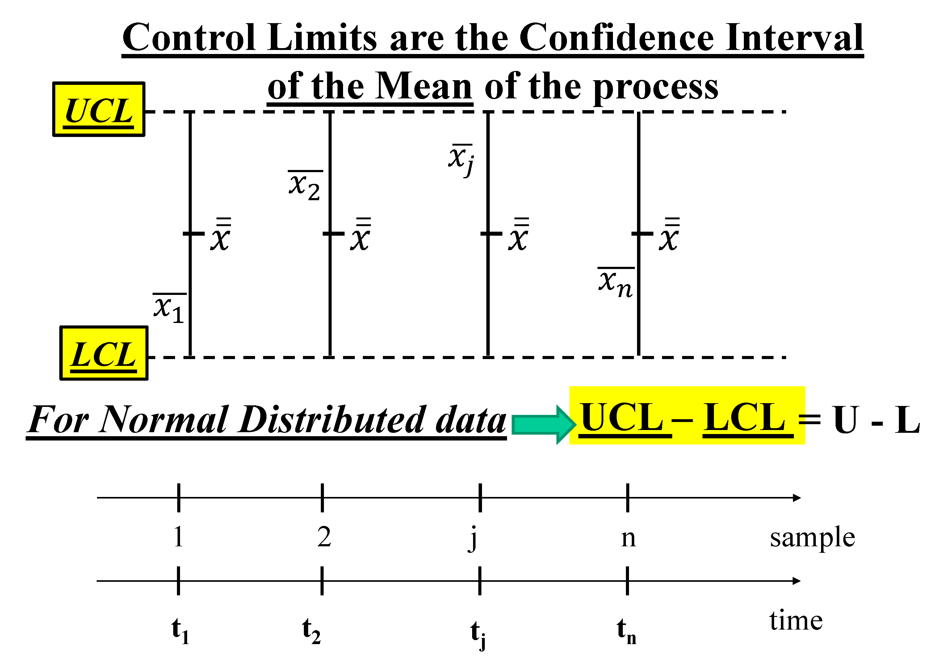
We said that (14) is a Probability Interval; IF we put in place of and in place of we get the CI of when a sample size k is considered for each , with CL=0.9973. The quantity is the mean of the standard deviations of each sample. This allows us to compare each (subsystem) mean , q=1,2, …, n, to any other (subsystem) mean r=1,2, …, n, and to the (Stand-by system) grand mean . If two of them are different the process is OOC. The quantities and are the limits of the Control Limits of the CC. When the Ranges Ri=max(xij)-min(xij) are considered for each sample we have , and , U, where the coefficients A2, D3, D4 are tabulated and depend on the sample size k [24,25,26,27,28,29,30,31,32,33,34,35].
The interval LCLX-------UCLX is the “Confidence Interval” with “Confidence Level” 1-α=0.9973 for the unknown mean of the Stochastic Process X(t) (Galetto 1981-2022).
The interval LCLR----------UCLR is the “Confidence Interval” with “Confidence Level” CL=1-α=0.9973 for the unknown Range of the Stochastic Process X(t) (Galetto 1981-2022). Notice that the Control Interval [Confidence Interval] UCLX-LCLX=U-L [Probability Interval, formula (14)] for normally distributed data and that LCLX can be obtained from L by substituting μ with ; the same for UCLX and U.
The error highlighted, the confusion between the Probability Interval and the Control Limits (Confidence Interval!) has NO consequences for decisions WHEN the data are Normally distributed, as hypothesised by Shewhart. On the contrary, it has BIG consequences for decisions WHEN the data are Non-Normally distributed as in the Excerpt 6. Notice!
Figure 9.
Control Limits LCLX----UCLX=L----U (=Probability interval), for Normal data.
2.5. Control Charts for TBE Data
We consider now, again, TBE (Time Between Event) data, exponentially or Weibull distributed. Quite a lot of authors (see Appendix A, “Garden …”) compute wrongly the Control Limits.
The previous section formulae are used also for NON_normal data (see Excerpt 6): for that, the NON_normal data are transformed “with suitable transformations” in order to “produce Normal data” (see Excerpt 6) and to apply those formulae (above).
Sometimes we have few data and then we use the so called “individual control charts” I-CC. The I-CC are very much used for exponentially distributed data: they are named “rare events Control Charts for TBE (Time Between Events) data”, I-CC_TBE (see Excerpt 6).
The author (FG) knew about the wrong way of dealing with I-CC_TBE since 1996 by reading the Montgomery book where he transformed the into Weibull data (approximately normal) following Nelson L. S. (J. Qual. Techn., 1994): he acted wrongly in all the later editions of the book. Any scholar who wants to learn Control Charts both with normal distribution and TBE can usefully read the book “Statistical Process Management” [35].
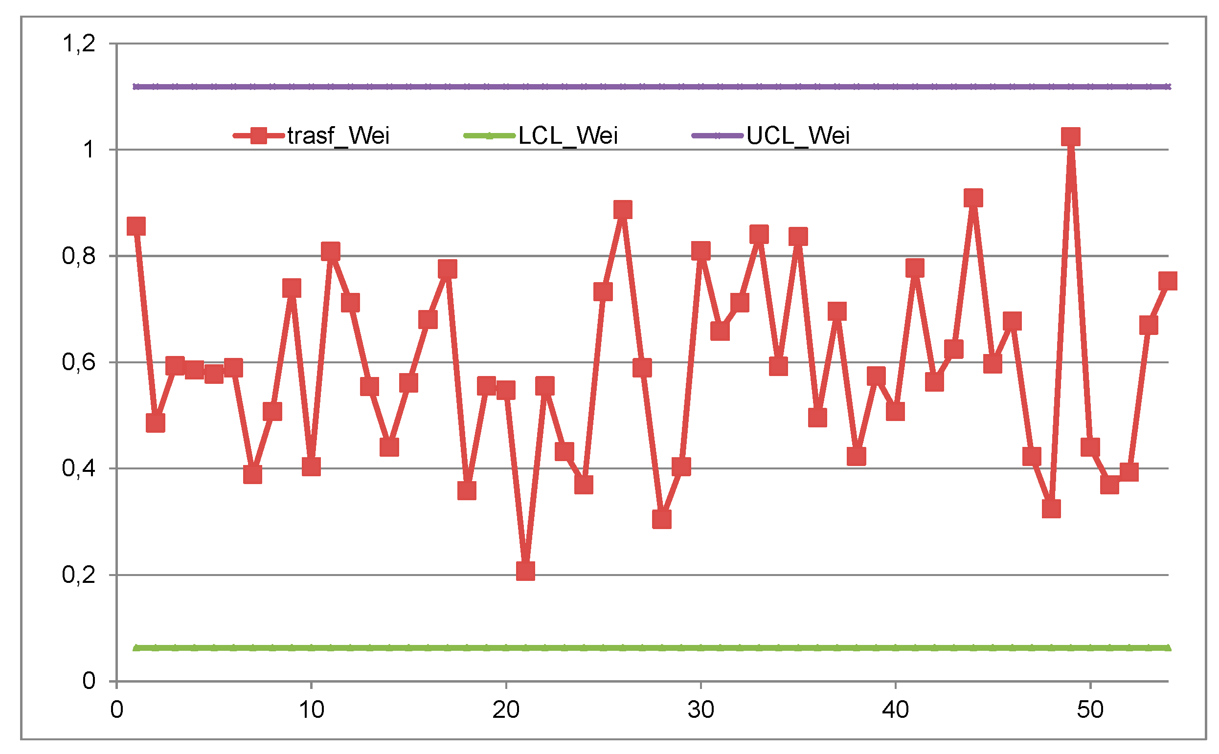
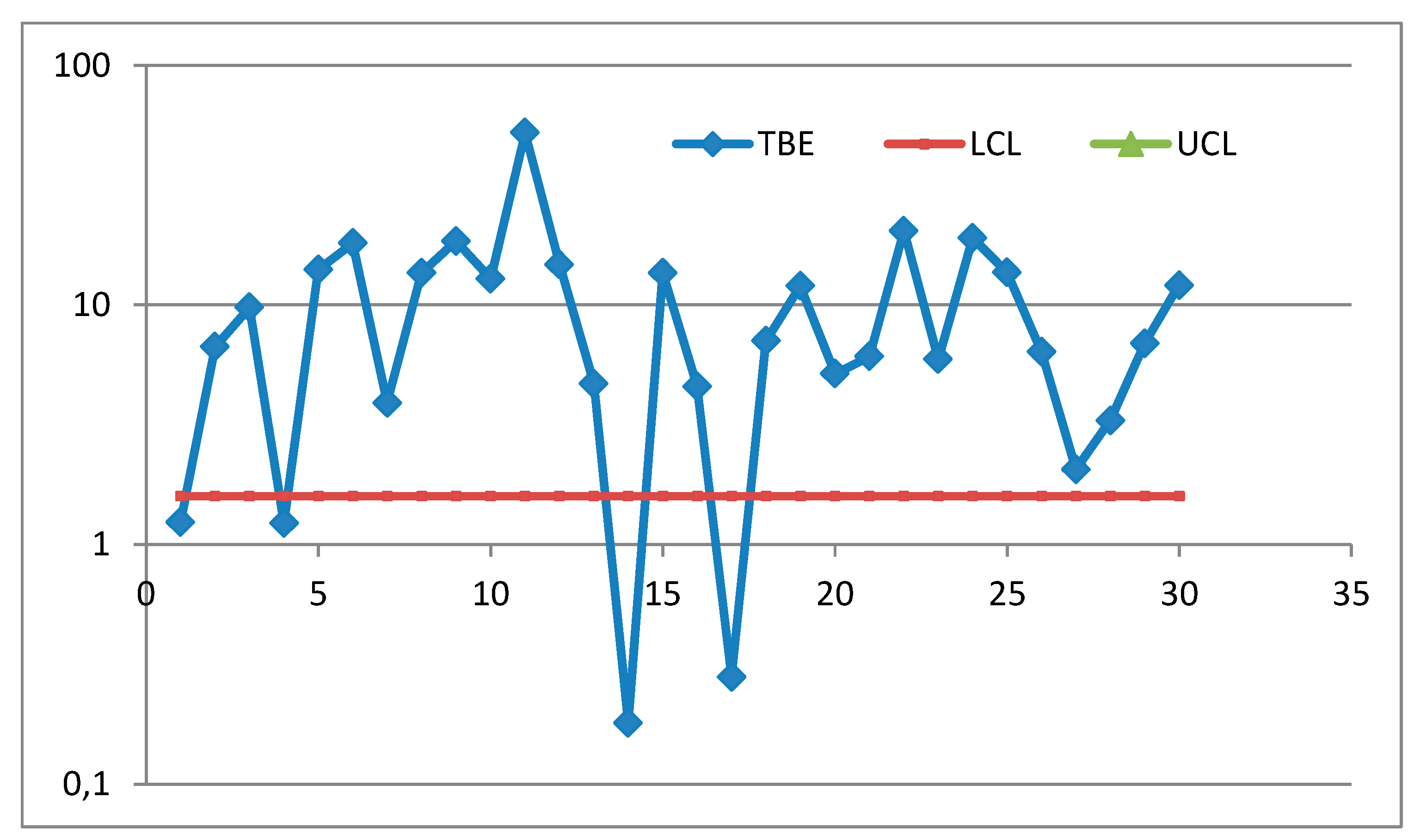
Several authors did the same as Montgomery did. See the Journal Operation Research and Decisions where the 3 authors, in their paper “An EWMA Control Chart for the exponential distribution” made the same error transforming the data into Weibull with β=1.36; the data are the “Urinary Tract Infection” (UTI) taken from a paper of two Minitab authors (Santiago & Smith) in their “Control charts based on the Exponential Distribution”, Quality Engineering;: their T Chart (Figure 11) shows the process IC: wrong decision; making the transformation we could draw the I-CC as in Figure 12 where the Control Interval=UCL-LCL=U-L=the Probability Interval. The process is again IC: wrong decision. It is NOT so if we analyse directly the TBE (Figure 13).
Using RIT (the Reliability Integral Theory of F. Galetto) we get the Figure 13 (vertical axis logarithmic, to let the OOC points evident). The process is OOC.
The problem with the authors in the “Garden…” is that hey do not care of Theory: they do not consider that THEORY MATTERS, in every field!
Figure 10.
Individual Control Chart (sample size k=1). Control Limits LCL----UCL=L----U (Probability interval), for Normal data.
Figure 10.
Individual Control Chart (sample size k=1). Control Limits LCL----UCL=L----U (Probability interval), for Normal data.
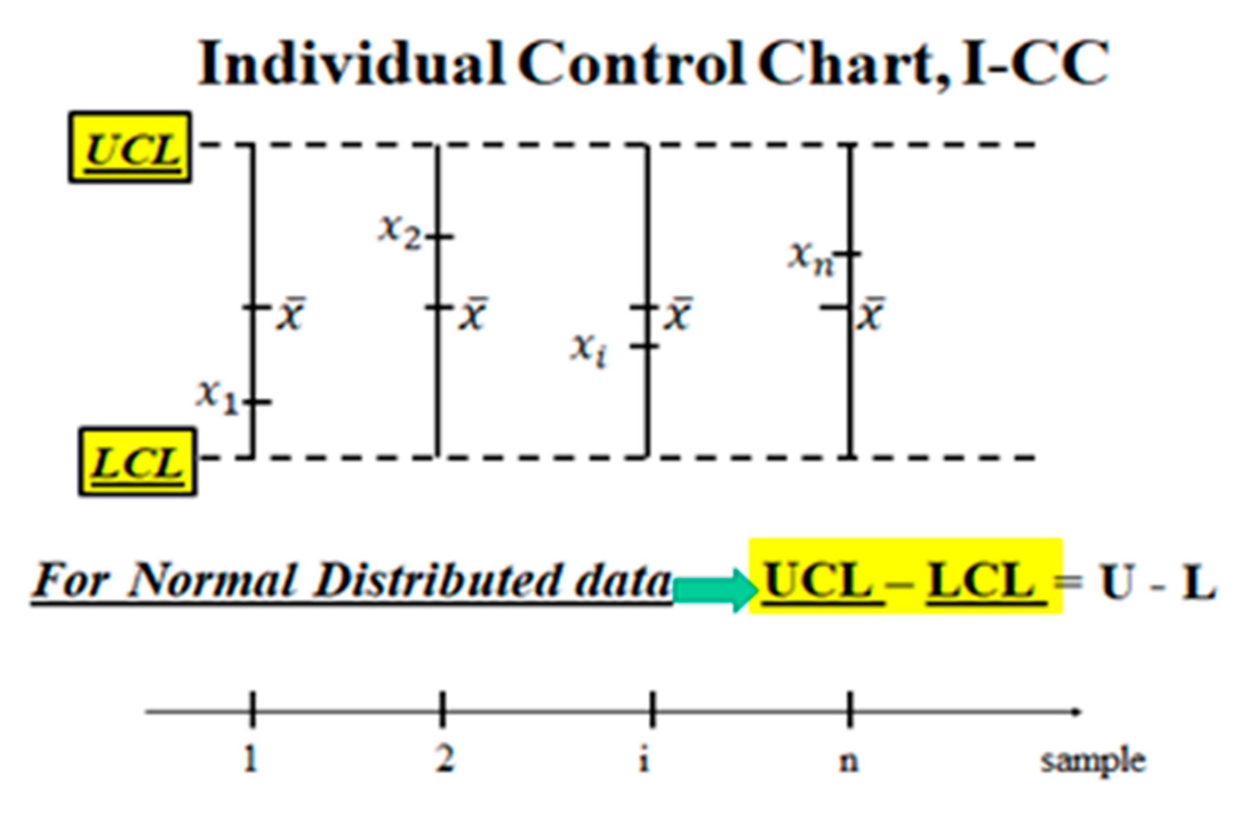
Figure 11.
Chart of Minitab authors’ paper data (Urinary), Minitab 19 used.
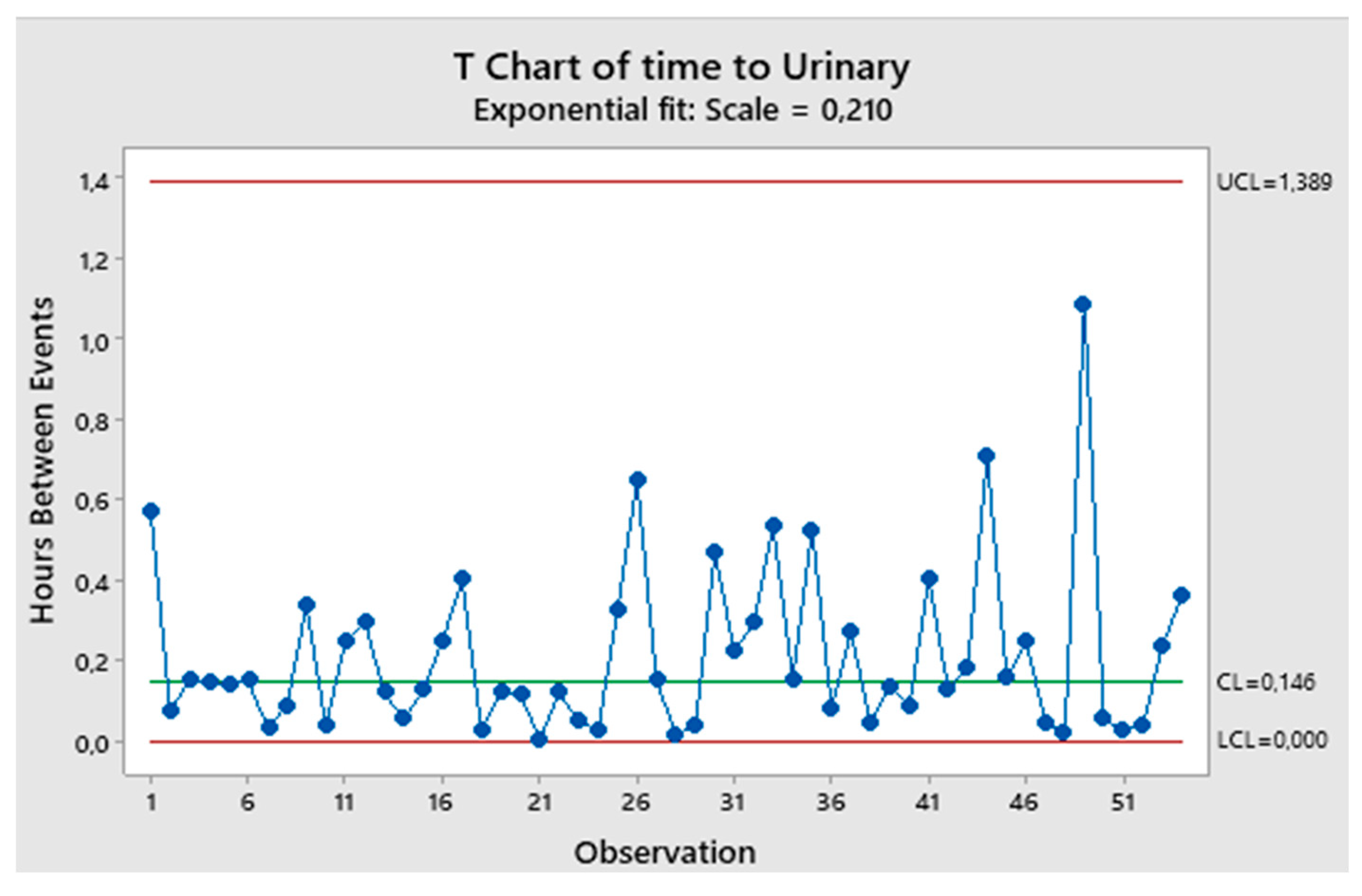
Figure 12.
I-CC of the UTI, transformed into Weibull data.
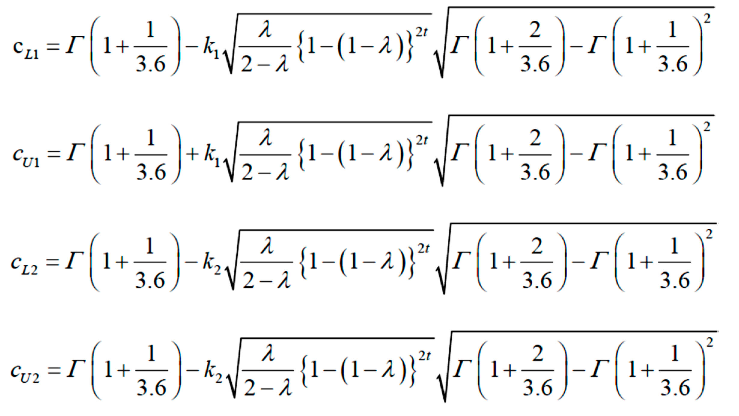
On the contrary, making the same error as Montgomery, the 3 authors transform the data into Weibull with β=1.36 and then they make an EWMA Chart with “double Control Limits” with the formulae , where with the “target of an IC process”:
Excerpt 7.
From the paper “An EWMA Control Chart …” (the k coefficients are to be suitably found…). Notice the errors in the formulae..
Excerpt 7.
From the paper “An EWMA Control Chart …” (the k coefficients are to be suitably found…). Notice the errors in the formulae..
See now the wrong I-CC in the figures 11, 12, 14; only the CC in the Figure 13 is right.
Figure 13.
I-CC of the UTI, y-axis logarithm mic. RIT used (F. Galetto).
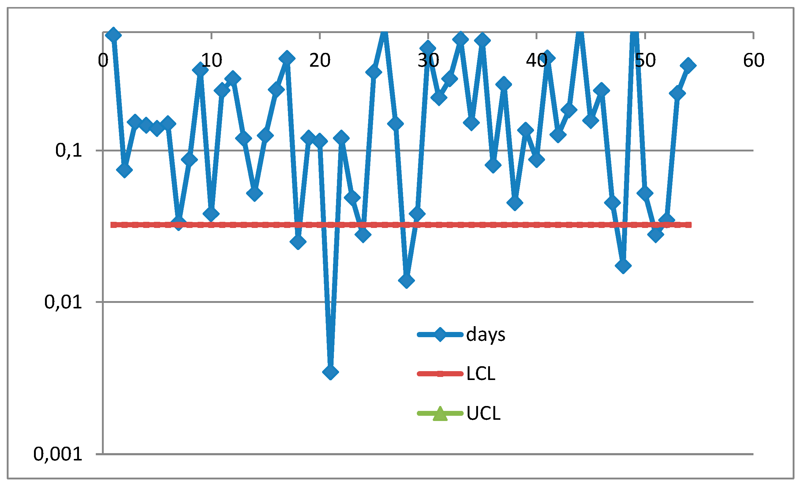
Figure 14.
EWMA (F. Galetto) of the UTI.
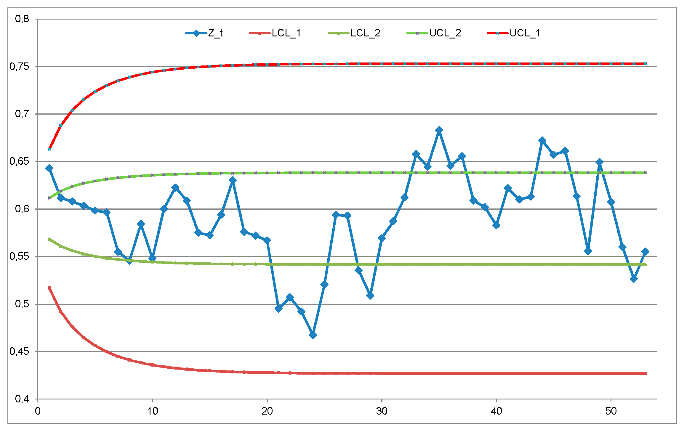
In the paper mentioned there is a figure: we did not find the data used for the target and the coefficients k. Hence, we used the target =0.59, coefficients k=-2.7, -0.8, 0.8, 2.7 and λ=0.2; we got the Figure 14.
Those authors made a mess; the Peer Reviewers did not analyse correctly the paper, and the Editors did not do their Job. The same as for all the papers in the “Garden …”. Remember Juran who mentioned the FG paper, at the Plenary Session of the EOQC Conference … [36]
3. Results
Now it is time to see the wrong formulae used by the “Garden …” authors. A smal sample in in the Excerpt 8.
Excerpt 8.
Typical statements in the “Garden full of errors …” where the authors name LCL, UCL what actually are the Probability Limits L and U.
Excerpt 8.
Typical statements in the “Garden full of errors …” where the authors name LCL, UCL what actually are the Probability Limits L and U.
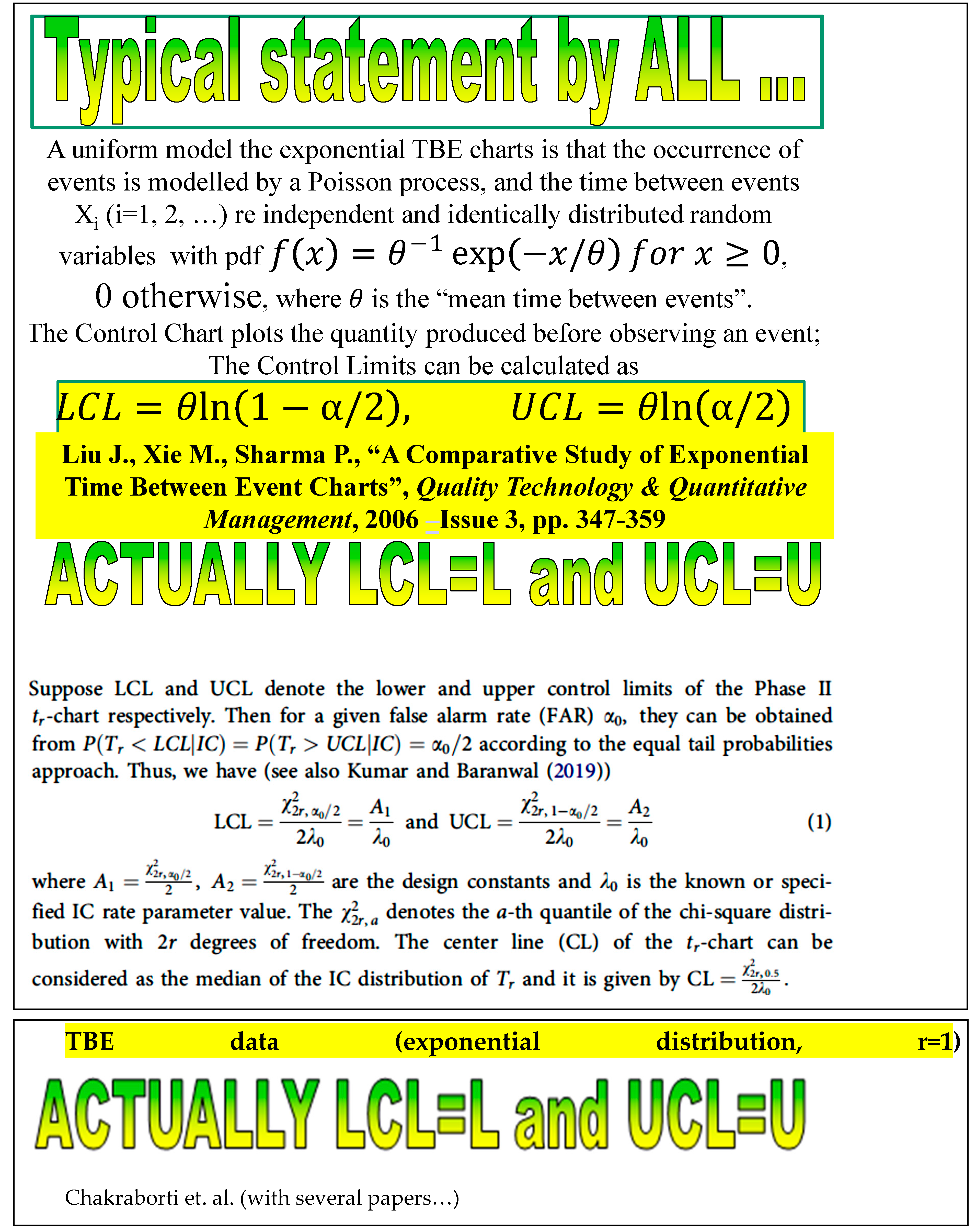
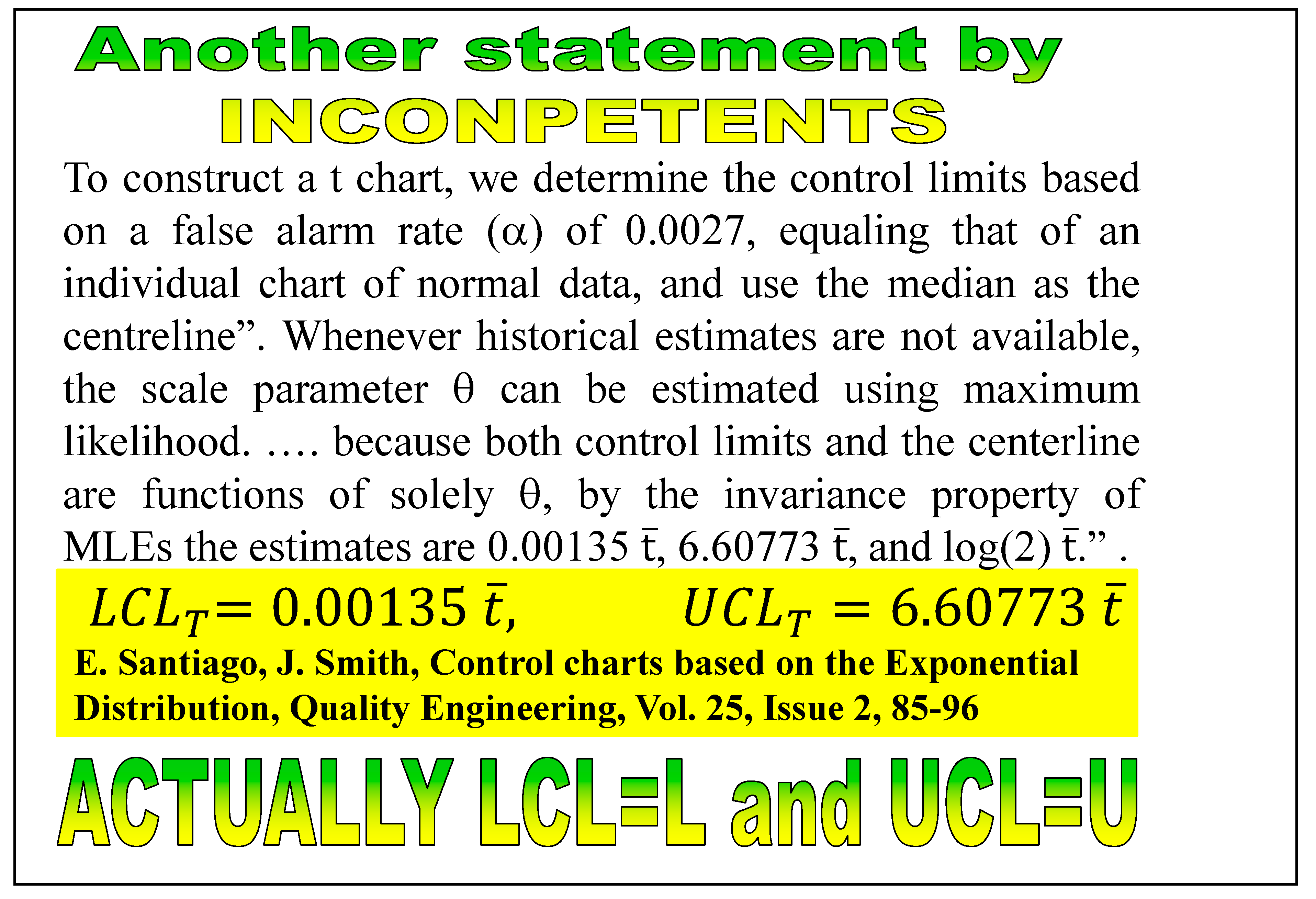
All the authors in the “Garden …” make the same error: they confuse the Probability Interval with the Control Interval in CCs (Confidence Interval!). The same happens for MINITAB, JMP, SAS, … software.
Now we see how RIT solves the I-CC_TBE with exponentially distributed data. Before we computed the Confidence Interval is CI=-------- of the parameter , using all the data with the “total of the data of the empirical sampleD (n=20)” and Confidence Level CL=. When we deal with a I-CC_TBE we have to consider the Figure 10 and compute the LCL and UCL through the empirical mean (mean observed time to failure /n) we only have to solve the two following equations with unknown LCL and UCL
similar to (13). For exponentially distributed data (15) become
The two equations (16) show clearly the errors of the authors in the “Garden …”. See on the left.
See the case by the Peer Reviewer chosen by the Editors of Quality and Reliability Engineering International about the Control Limits for Individual Control Charts with Exponentially distributed data and compare the results:
Khakifirooz, M., Tercero-Gómez, V. G. and Woodall, W. H. (2021). The role of the normal distribution in statistical process monitoring, Quality Engineering 33(3), 497–51
3.1. Some Papers from the “Garden …”
Let’s see some other few cases from the “Garden …”.
Consider the paper Box-plot based Control Charts [by Chakraborti (same author in excerpt 5.) et al.), Quality and Reliability Engineering International, 2011.
Figure 15.
I-CC of Montgomery data analysed by Chakraborti (with α0=0.01).
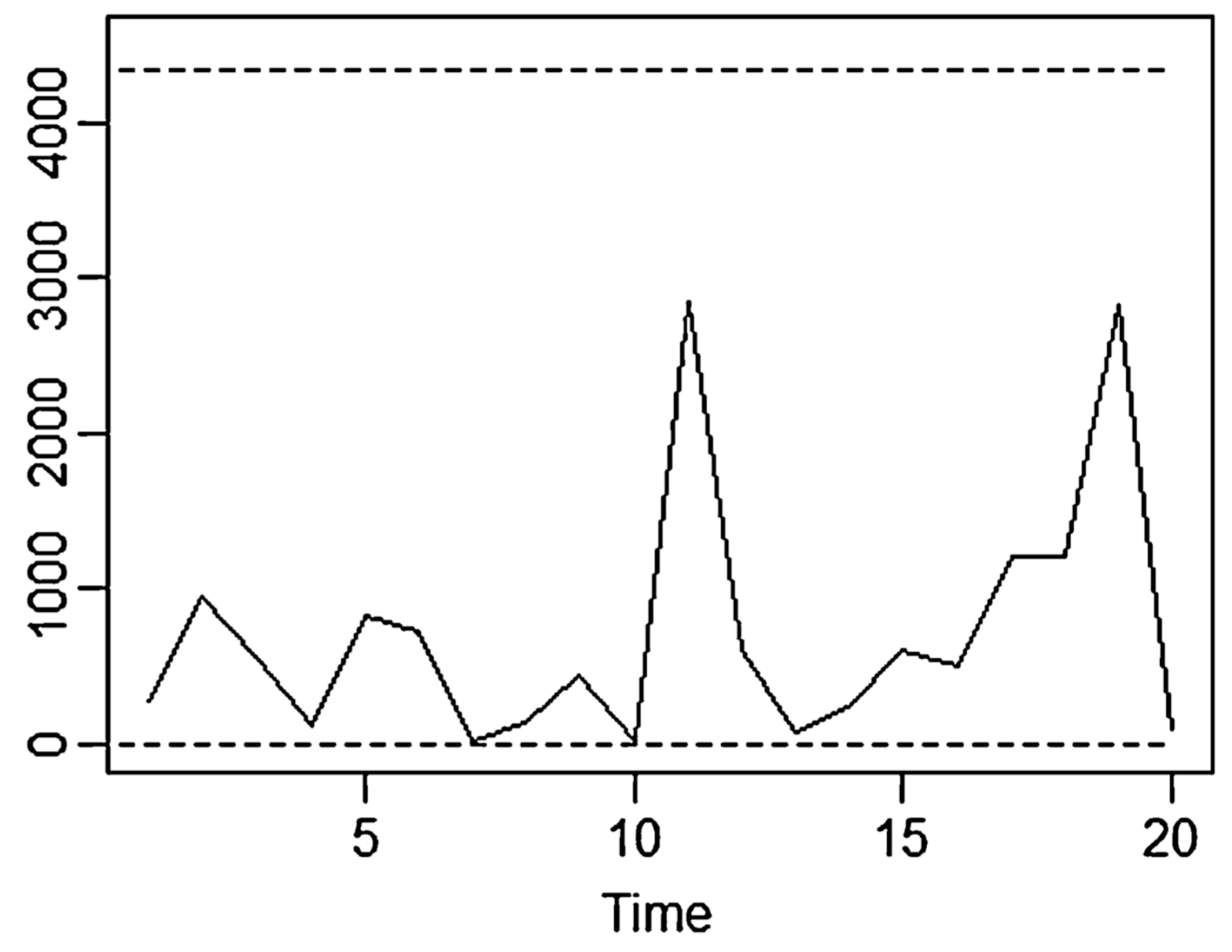
Figure 16.
T Chart of Table 1 data. Minitab 19&20&21 used (F. Galetto).
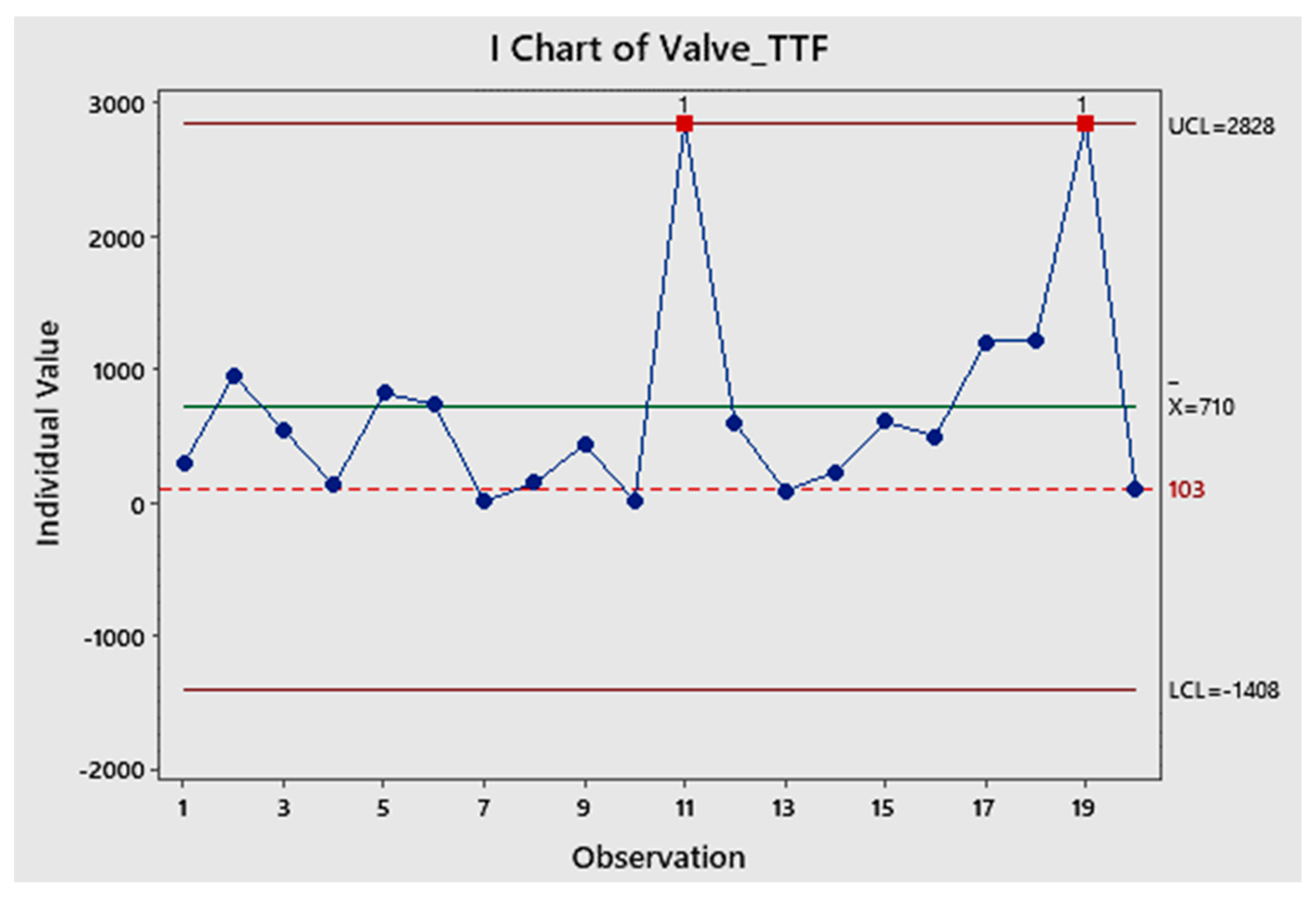
Notice QREI again], where the lifetime data (“valves TTF”) the same as in Montgomery, 2013, page 334) are analysed; the authors use the median (instead of the mean) and the interquartile range (instead of the ranges). The two authors define the control limits with a form similar to Shewhart (but significance level α0=0.01): the process (Figure 15) is found IC, as did Montgomery.
Using the T Chart of Minitab (which makes use of the wrong formulae, devised by Santiago & Smith) we can find the Figure 16: the process is found IC (as in Figure 15, Chakraborti, and as Montgomery).
By using Minitab , one finds the Figure 17 (with wrong OOC as in the Excerpt 8, as happened in the Excerpt 6): UCL and LCL are wrong, while the dotted line (found with RIT) is the correct LCL. Compare figures 16 and 17: only the dotted line is the right correct LCL, allowing taking correct decisions: huge costs of DIS-quality applications/decisions by Minitab Clients, caused by Minitab wrong methods.
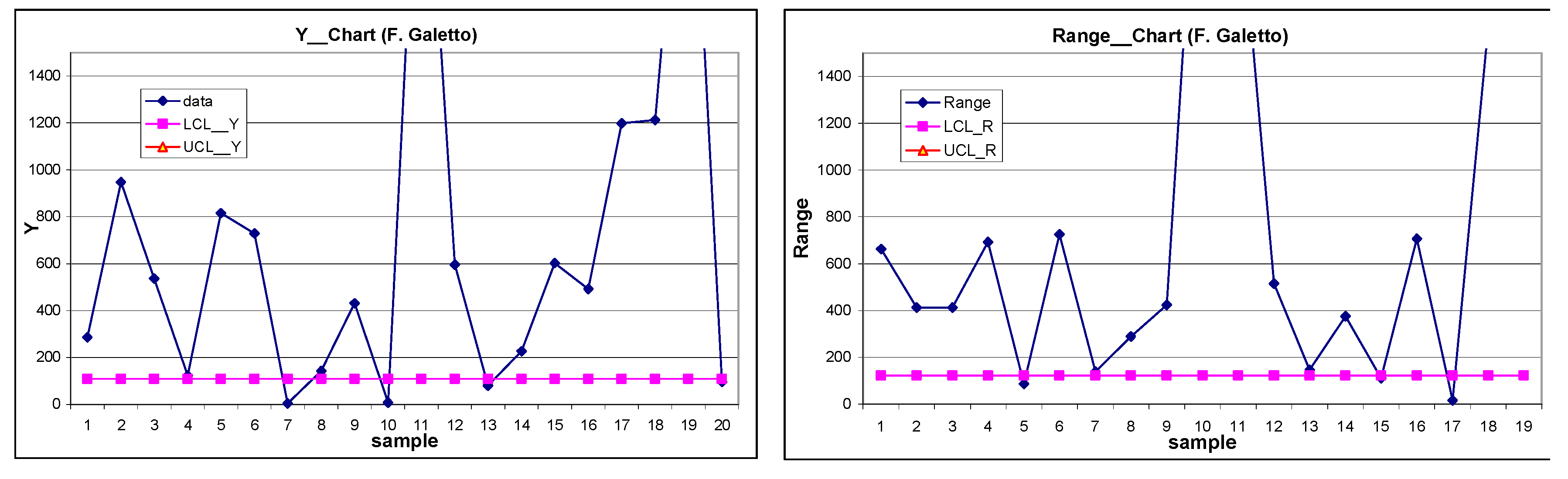
The process is OOC. The reader can see easily from figures 17, 18. The ranges too are OOC.
Figure 17.
(F. Galetto) I Chart (Control charts) for valves data (Minitab 19&20&21 used). The dotted line is the right correct LCL when RIT is used; the UCL is wrong.
Figure 17.
(F. Galetto) I Chart (Control charts) for valves data (Minitab 19&20&21 used). The dotted line is the right correct LCL when RIT is used; the UCL is wrong.
It should be clear that Managers, Professors and Scholars must use the Theory. The author, for many years, has been showing the many drawbacks present in various books and papers: unfortunately, he had little success; only few understood (one was Juran at 1989 EOQC Conference, Vienna).
Figure 18.
(F. Galetto) Scientific Control Charts for valves data [related to the data and control charts in Montgomery books]. RIT is used.
Figure 18.
(F. Galetto) Scientific Control Charts for valves data [related to the data and control charts in Montgomery books]. RIT is used.
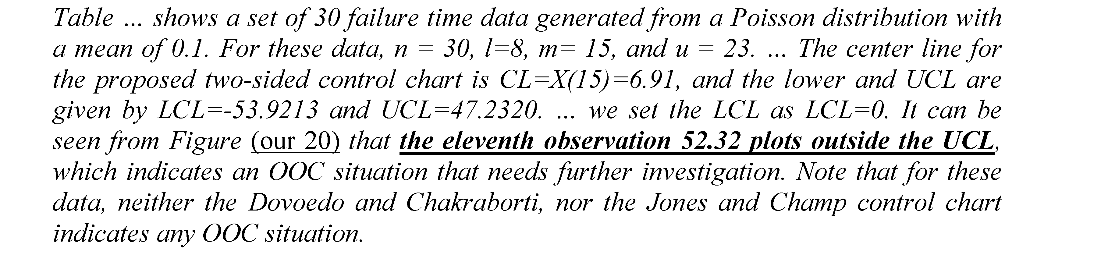
Now we see another paper in the “Garden…” (found online, 2021) “Improved Phase… for Monitoring TBE” [Chakraborti (same author above et al.) published by QREI (again). The two authors provide a wrong solution (found neither by the Peer Reviewers nor by the Editor!). Nevertheless, they write in their Acknowledgements: … The authors would like to thank Dr. Douglas Montgomery, Co-editor, for his interest and encouragement. In the authors’ Abstract, we read
and
See their Concluding remarks.
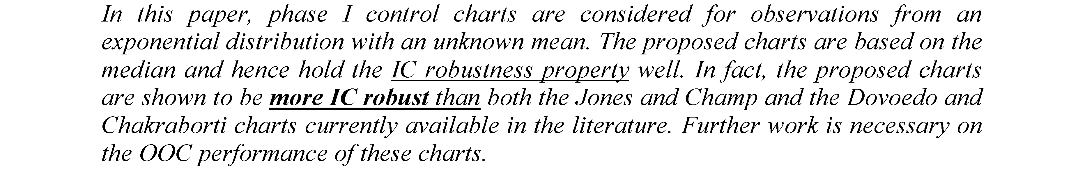
We agree that “Further work is necessary on the OOC performance of these charts”: the further Work must be to STUDY (see Deming!).
The wrong CC (in Figure 19) shows a “false” OOC situation and various “false” IC…
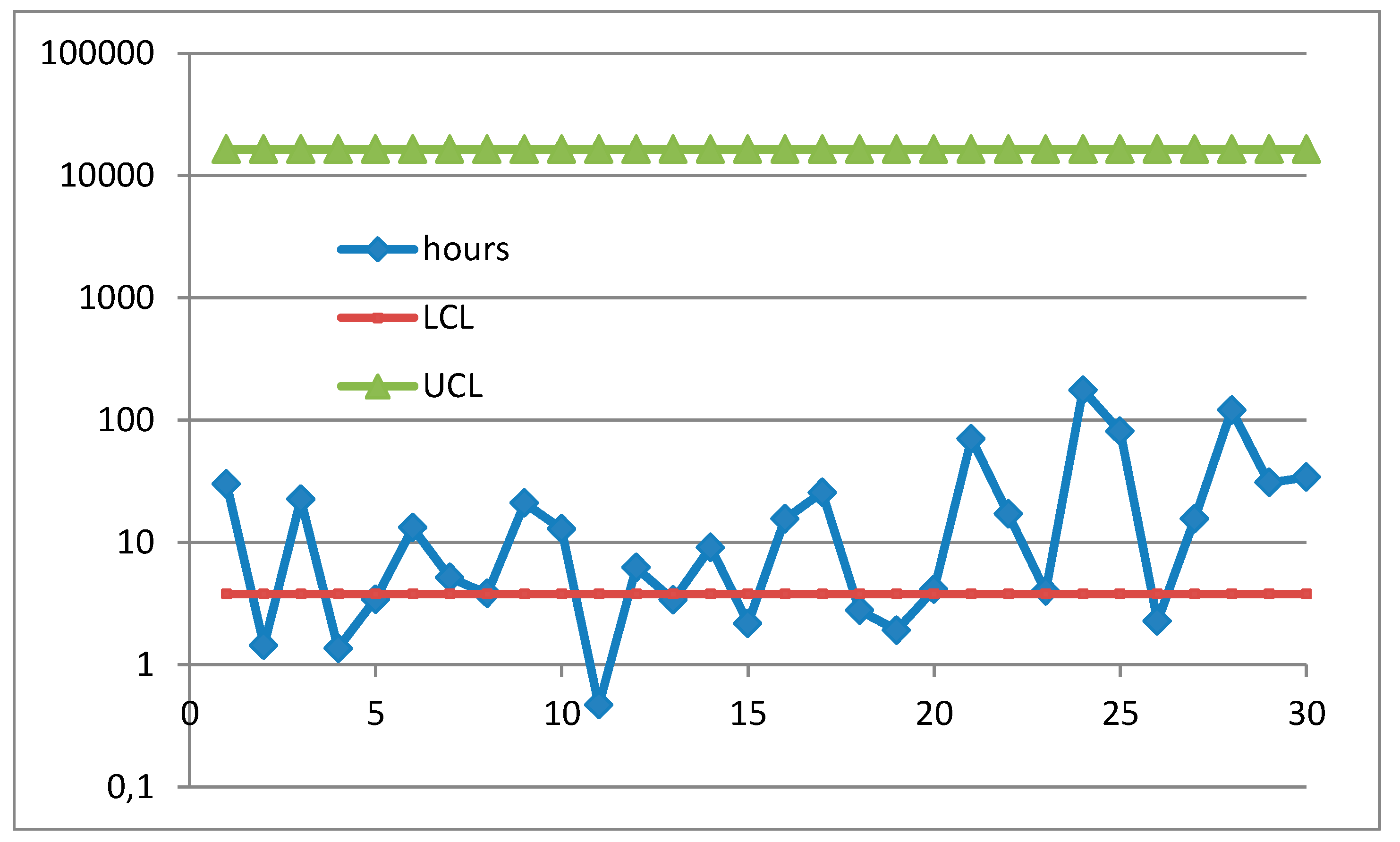
Using RIT as done previously the n=g*=30 TBE can be considered as the “transition times” between states of a stand-by system of 30 units: the Up-states are 0, 1, …, 29, and 30 is the Down-state; ti is the “time to failure ” from state i-1 to state i. R0(t|θ) is the system reliability for the interval 0----t, given θ, and it is, as well, the Operating Characteristic Curve of the reliability test, given t. At the end of the test, we know tO the observed Total Time on Test.
Figure 19.
Control Chart from “Improved Phase… for Monitoring TBE”.
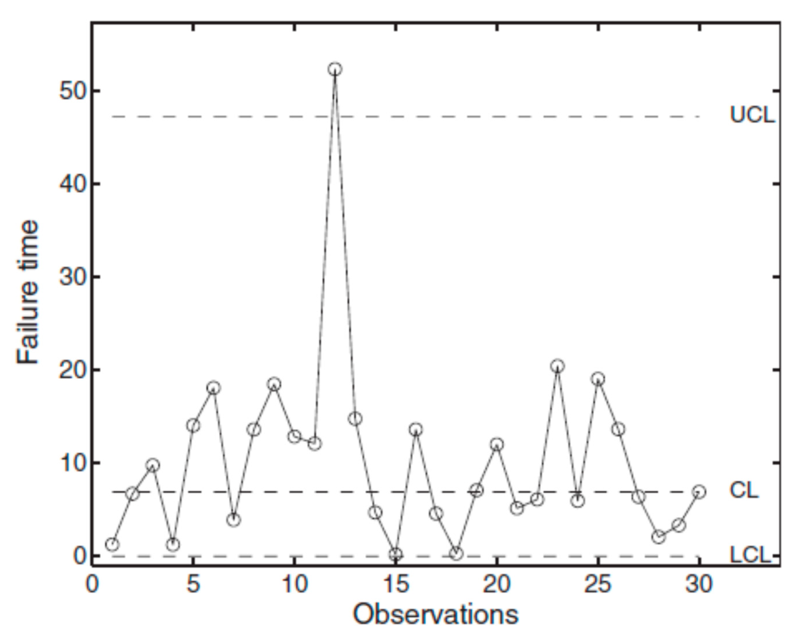
We want to analyse if the “individual” TBE are significantly different from the “mean observed time to failure” tO/n. The Control Limits are the values satisfying the two equations (13) with tO replaced by tO/n, that is two equations (15 and 16) for any single unit; so, we have 30 Confidence Intervals [all equal, by solving formulae (16)], given and CL=1-α.
Figure 20.
Control Chart of the data from “Improved Phase… for Monitoring TBE”; vertical axis logarithmic; UCL is >100. RIT used (F. Galetto).
Figure 20.
Control Chart of the data from “Improved Phase… for Monitoring TBE”; vertical axis logarithmic; UCL is >100. RIT used (F. Galetto).
Compare the figures 19 and 20: it is clear that the I-CC_TBE from “Improved Phase… TBE” presents 5 errors about OOC; the paper is wrong.
Also consider the paper Some effective control chart procedures for reliability monitoring published in Reliability Engineering & System Safety. Again, WRONG Control Limits! The authors Xie et al. the “Time between failures of a component”. They do not realise that at least 20% of the data are OOC (Figure 21), a very good result for a PR paper! All the people involved did not know the Theory. "It is necessary to understand the theory of what one wishes to do or to make." (Deming 1996) T Charts and the “Garden…” methods make the users to take wrong decisions...
Figure 21.
I-CC_TBE of Xie TBF data in “Some effective … for reliability Monitoring”; vertical axis logarithmic; RIT used (F. Galetto).
Figure 21.
I-CC_TBE of Xie TBF data in “Some effective … for reliability Monitoring”; vertical axis logarithmic; RIT used (F. Galetto).
Also, see a paper in (Multidisciplinary Open Access) IEES Access 2017, “EWMA Control Chart For Rayleigh Process With Engineering Applications (Alduais, Khan)”. At the end of the Abstract, we read the fantastic statements
“An application of the REWMA chart on simulated data also reveals that the proposed chart is highly sensitive to smaller and persistent shifts in the scaling parameter of Rayleigh distribution. Finally, an example from real-life has been presented to illustrate the importance of the suggested chart.”
Figure 22.
Proposed CC, ball bearing data [EWMA of of 8 samples, size 3)].
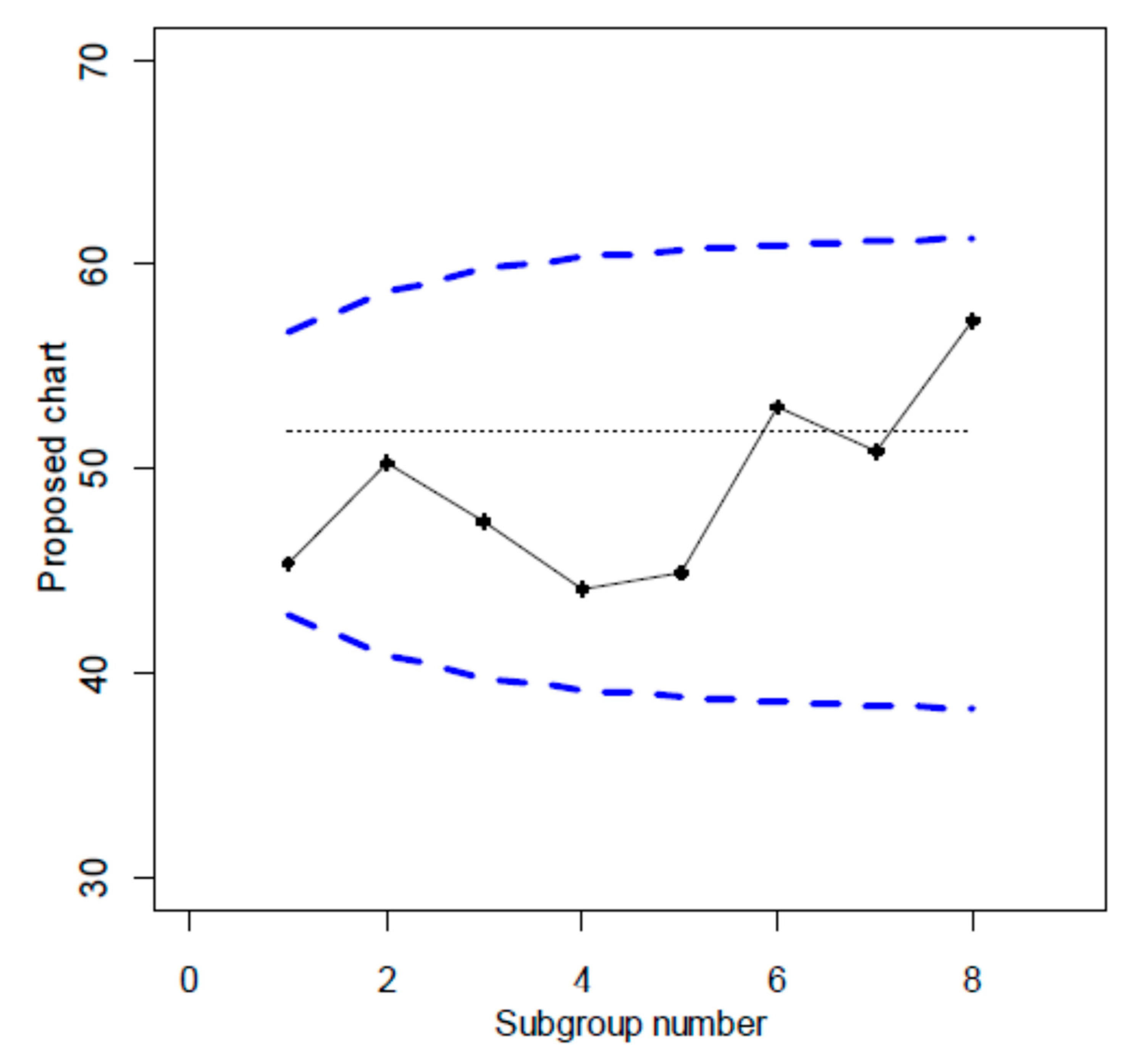
They consider the TTF (Time to failure, Rayleigh distributed) of 24 bearings (8 samples of size 3). The process of the 8 samples is IC (Figure 22) by their “theory”. On the contrary, the process is OOC [using RIT], both for the 24 Individuals (Figure 23) and the 8 samples (Figure 24).
The two authors claim in their Conclusions: “Simulation analysis also indicates the considerable improvement of the REWMA chart over the existing procedure in detecting shifts of smaller sizes in the study parameter”.
We think that the readers agree will not agree on that, by seeing the application (real) on the Ball Bearing failure data: the authors “detect shifts” but do not detect OOC… (Figure 23 and Figure 24).
Figure 23.
CC of the 24 Individuals TTF, RIT used.
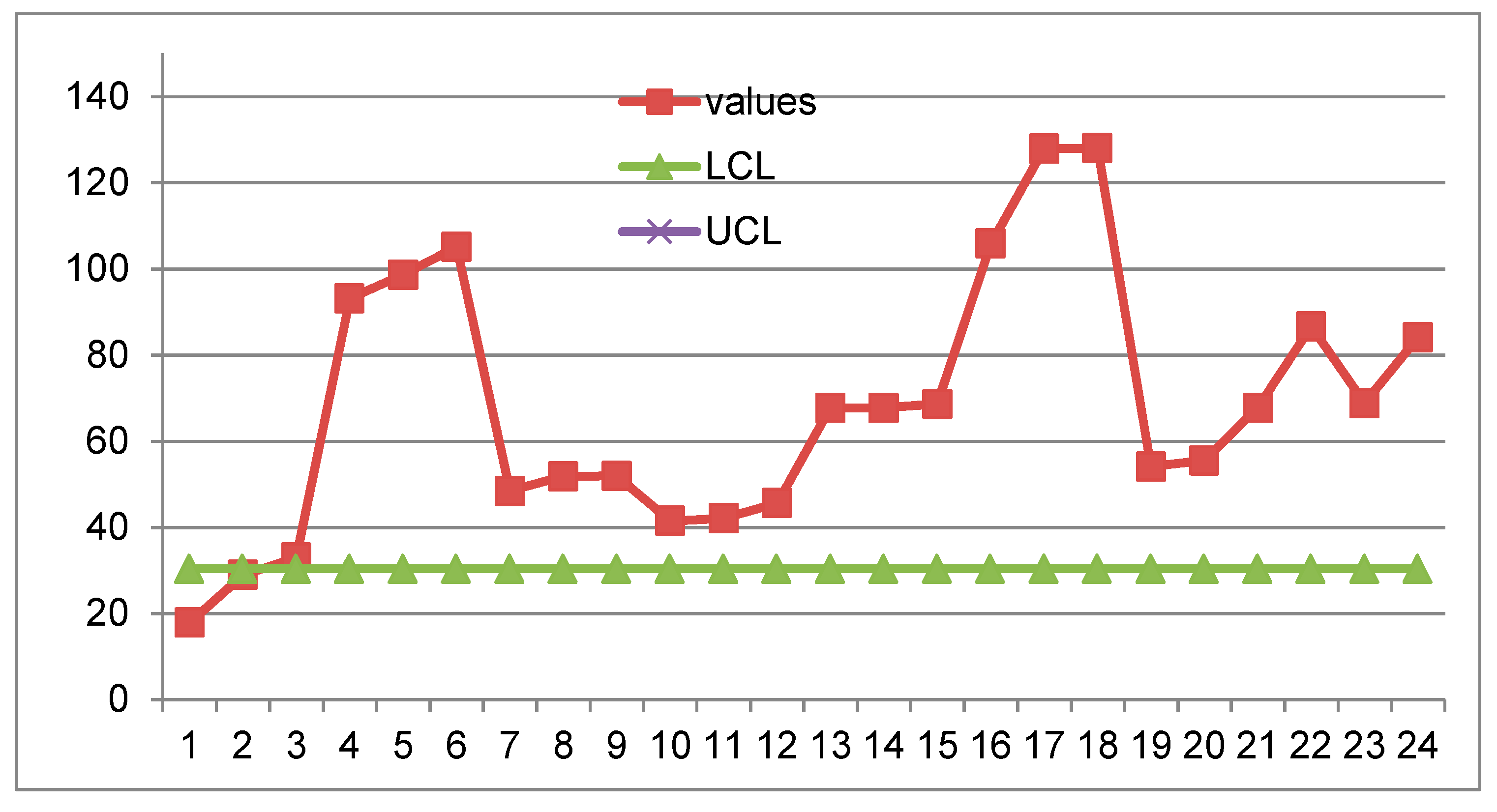
Figure 24.
CC for ball bearing data [ of the 8 samples], RIT used.
Last case: two papers (The length-biased weighted exponentiated inverted Weibull distribution, Cogent Mathematics, 2016, The Weighted Exponentiated Inverted Weibull Distribution, Journal of Informatics and Mathematical Sciences, 2017),
Excerpt 9.
From the paper “The length-biased weighted exponentiated inverted …”.
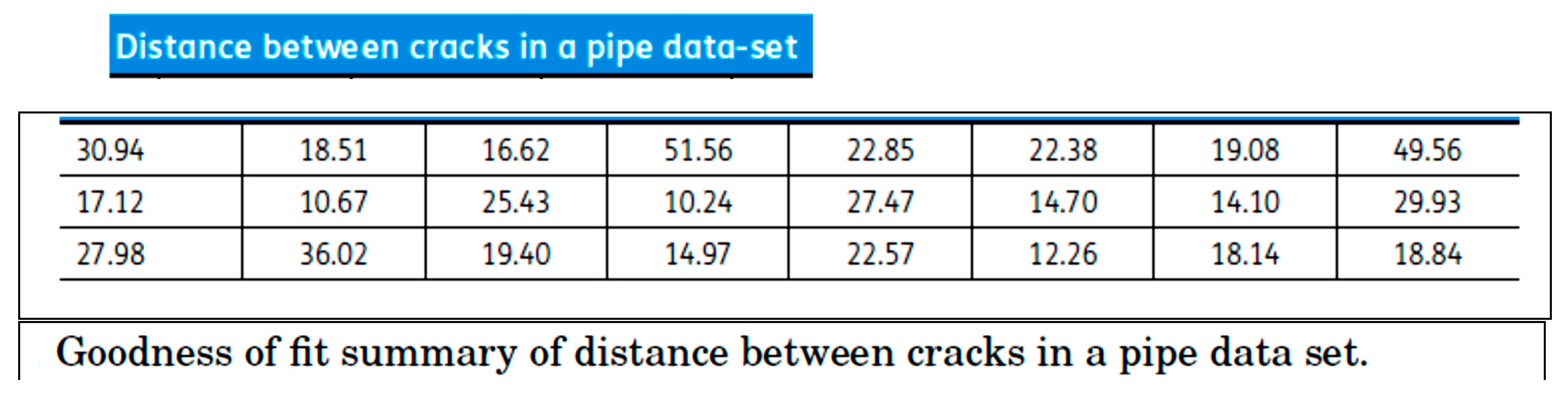
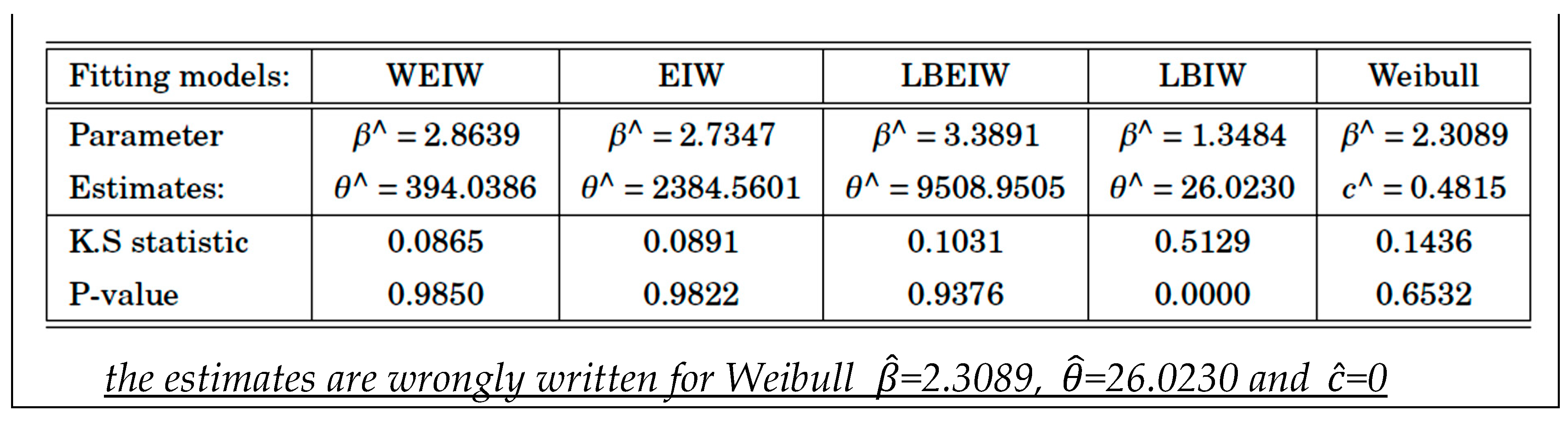
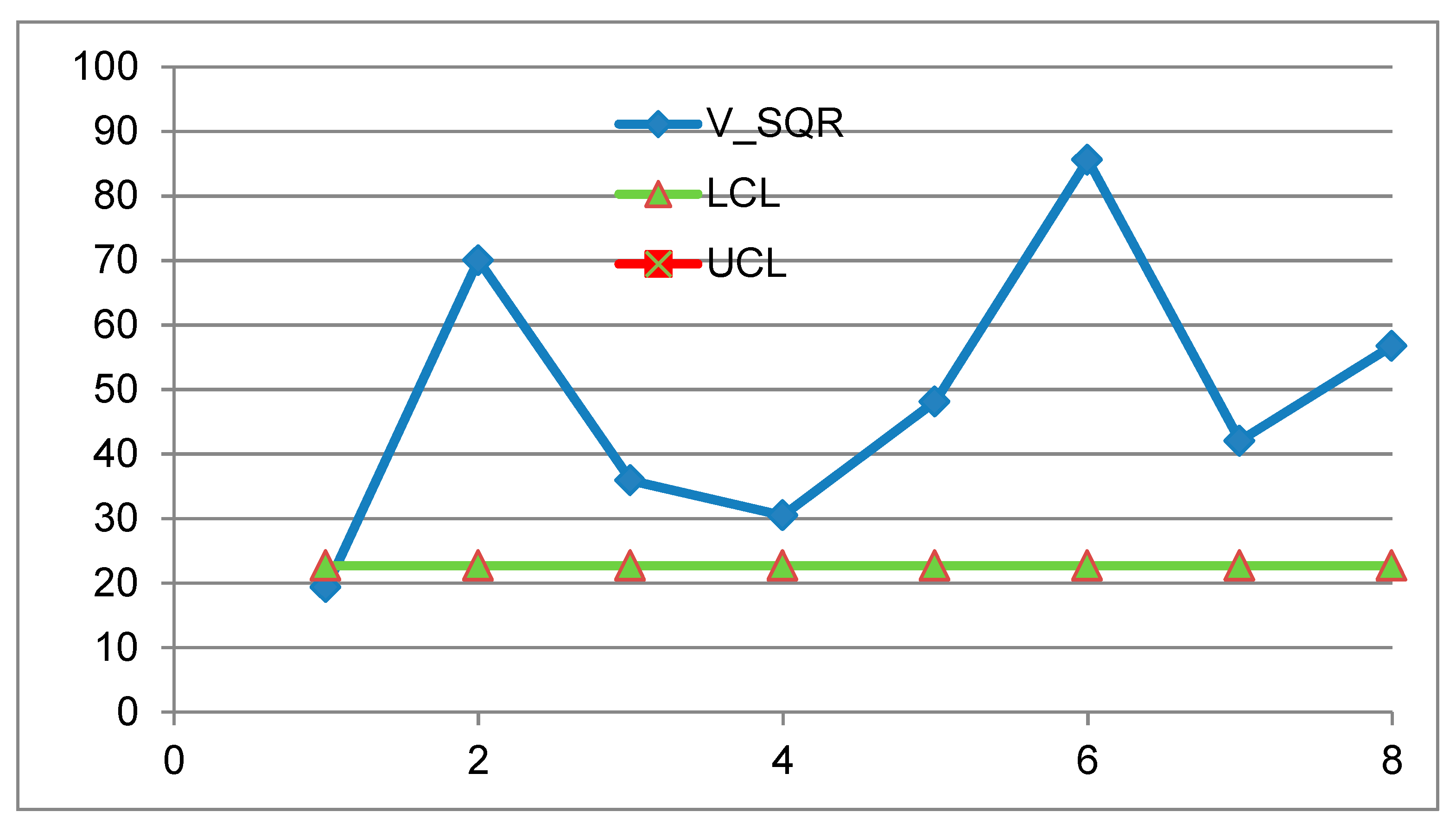
The papers deal with the same data, on the “distance of cracks in a pipe data-set”: same subject and the same real data as an application: they are in Excerpt 9, with the estimates of the density . The estimates of the parameters are (by the authors): =1.4256, =100.7943 and =1.4857. Notice that there is NO Confidence Interval… The authors do not provide any way to do that… When c=0 we get Length-Biased Exponentiated Inverted Weibull pdf (LBEIW), with estimates of the parameters (by the authors): =3.3891, =9508.9505, =0. NO Confidence Interval and not any way to find it…
A question arises: do the data of Excerpt 9 show a process In Control? In the papers there is no way to assess that. Using RIT, we find that the process is OOC for the 24 Individuals (Figure 25). Again, Authors, Peer Reviewers and Editors were wrong!
Also consider the paper On designing a new control chart for Rayleigh distributed processes with an application to monitor glass fiber strength published in Communication in Statistics- Simulation and Computation, January 2020. Again, WRONG Control Limits! The authors M. Pear Hossain et al. consider the “data on strength of 15 cm glass fibers”. They write:
Excerpt 10.
From the paper “On designing a new control chart … to monitor glass fiber strength.”.
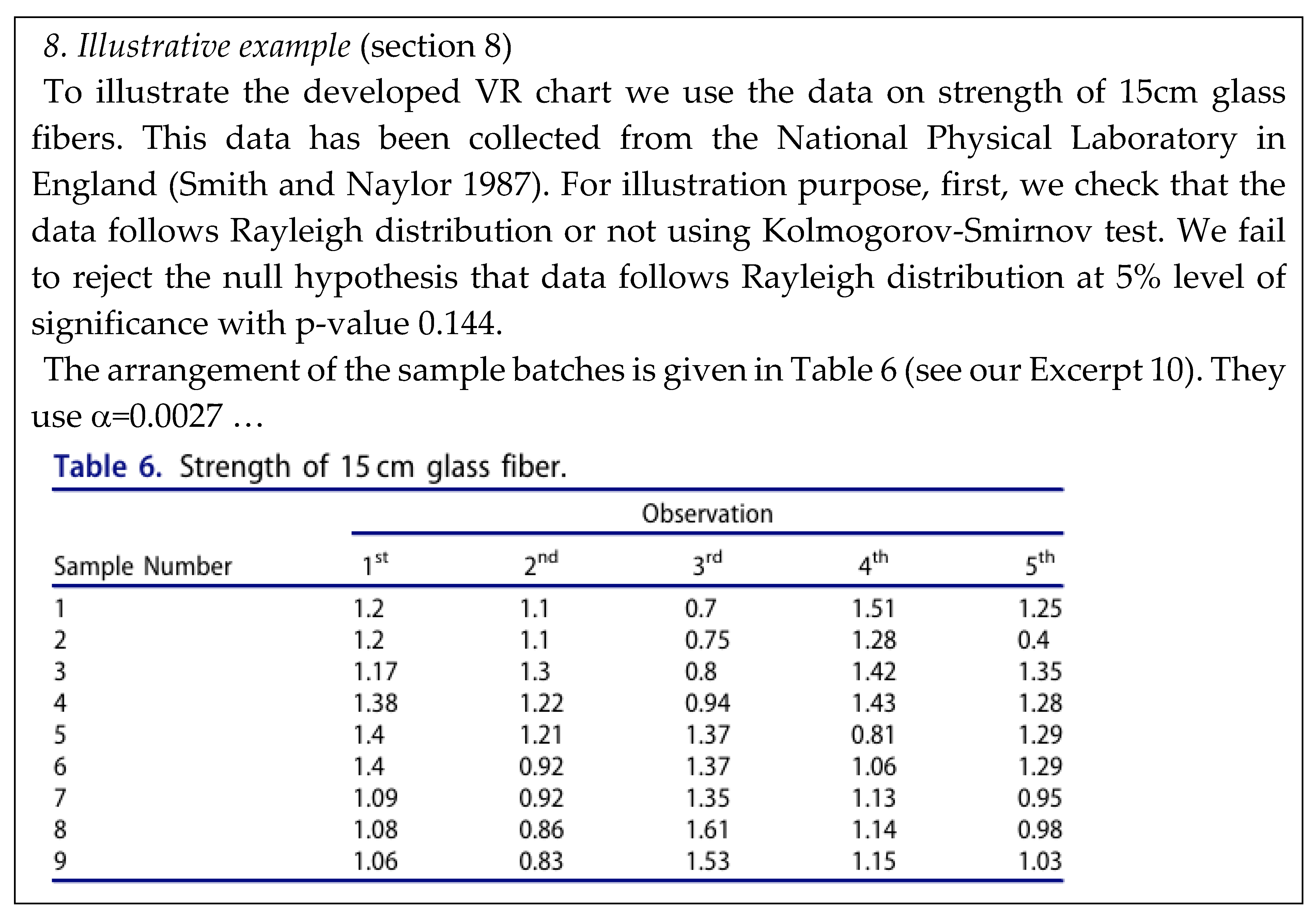
Notice the authors’ statement “We fail to reject the null hypothesis that data follows Rayleigh distribution at 5% level of significance with p-value 0.144.”
According [19] the Rayleigh distribution can be considered a Weibull distribution with β=2 (shape parameter). Analysing the data in Excerpt 10, we find that β=5.59, with a Confidence Interval CI=[3.81, 8.86] at CL=99.5%; the value 2 is not comprised in the CI: hence the distribution is not the Rayleigh distribution (also for CL=95%).
All the authors’ considerations are not valid for their Illustrative example (section 8), that is our Excerpt 10; they find that the “process is IC”.
Analising the data with RIT we get the Figure 26: the process is OOC, using the correct distribution and directly the data in our Excerpt 10.
Analising the data with the Normal distribution (a Weibull with β=5.59 can be approximated by the Normal ) we get the Figure 27: now the process is IC … as it was found by the authors with the Rayleigh distribution!
Figure 26.
CC of the Individuals (from the paper “On designing a new control chart … to monitor glass fiber strength”), RIT used.
Figure 26.
CC of the Individuals (from the paper “On designing a new control chart … to monitor glass fiber strength”), RIT used.
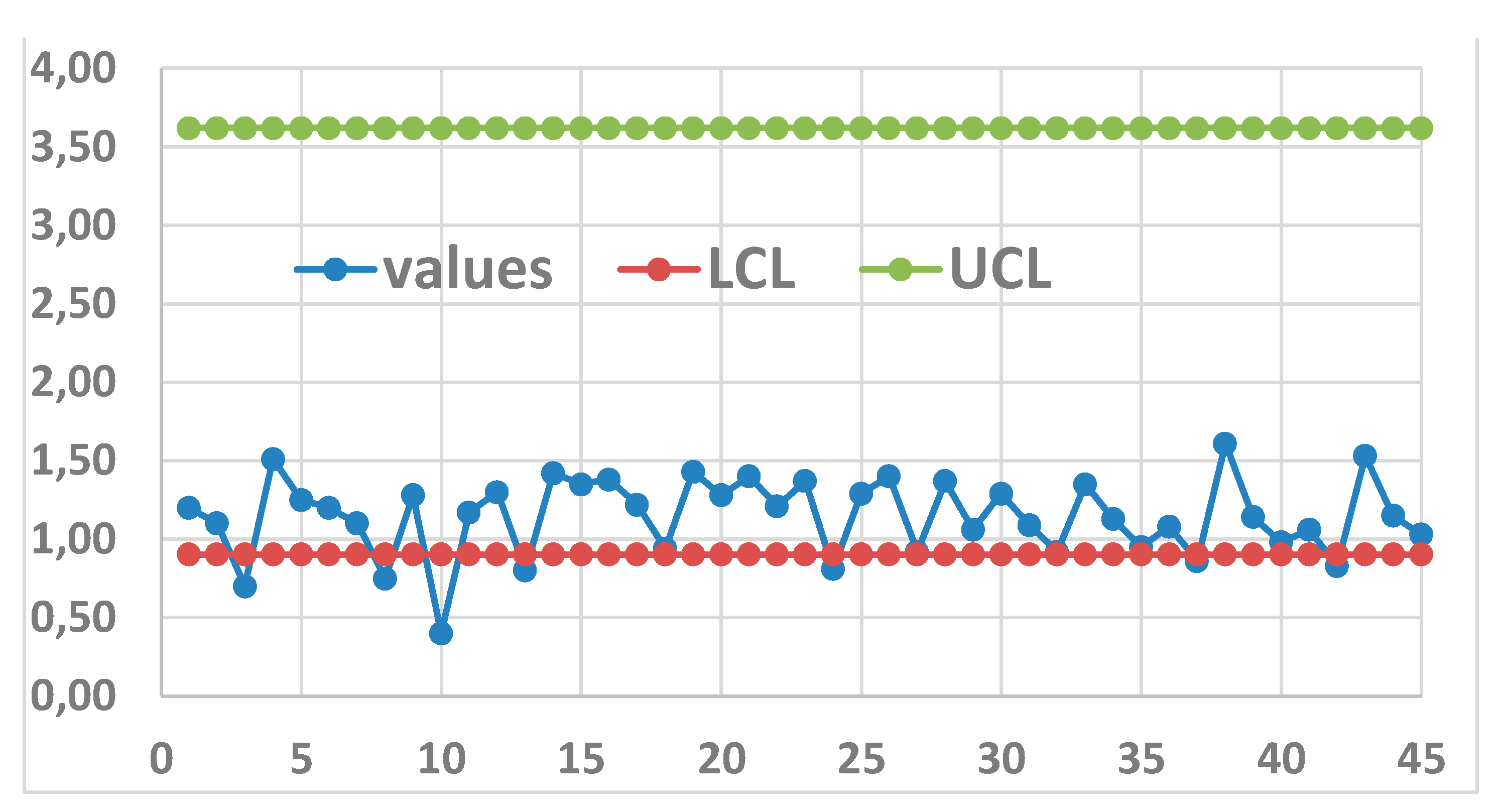
Figure 27.
CC of the samples with sample size 5 (from the paper “On designing a new control chart … to monitor glass fiber strength”), Normal distribution used.
Figure 27.
CC of the samples with sample size 5 (from the paper “On designing a new control chart … to monitor glass fiber strength”), Normal distribution used.
3.2. RIT and the Duane Method
We found this method in the software Minitab 19&20&21.
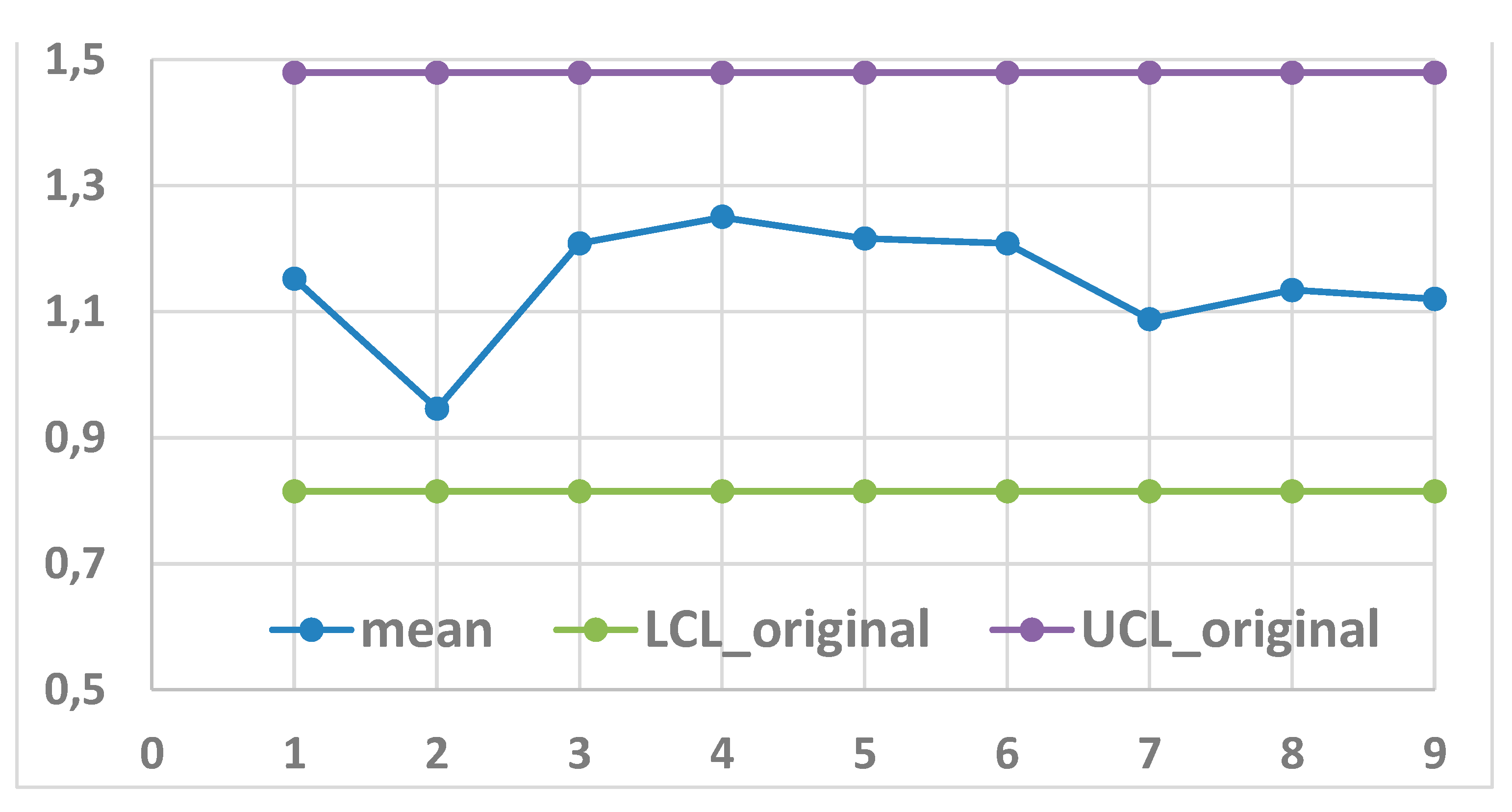
Minitab provides the data on “repairable air-conditioners” and a graphical picture of them [see Figure 28], and computes, the mean number of failures up to time t [M(t) function], of the 13 repairable systems: M(t)=E[N(t)]; they do not give any “theory” to interpret the results; they only inform us that (1) M(t) is interpolated by a model named “power law” (t/η)β, with β=shape parameter and η=scale parameter, and (2) the MLM (Maximum Likelihood Method) is used. No “Reliability Theory” is provided by Minitab: this is extremely dangerous and costing.
They say (with figures):
Figure 28.
13 repairable air-conditioners.
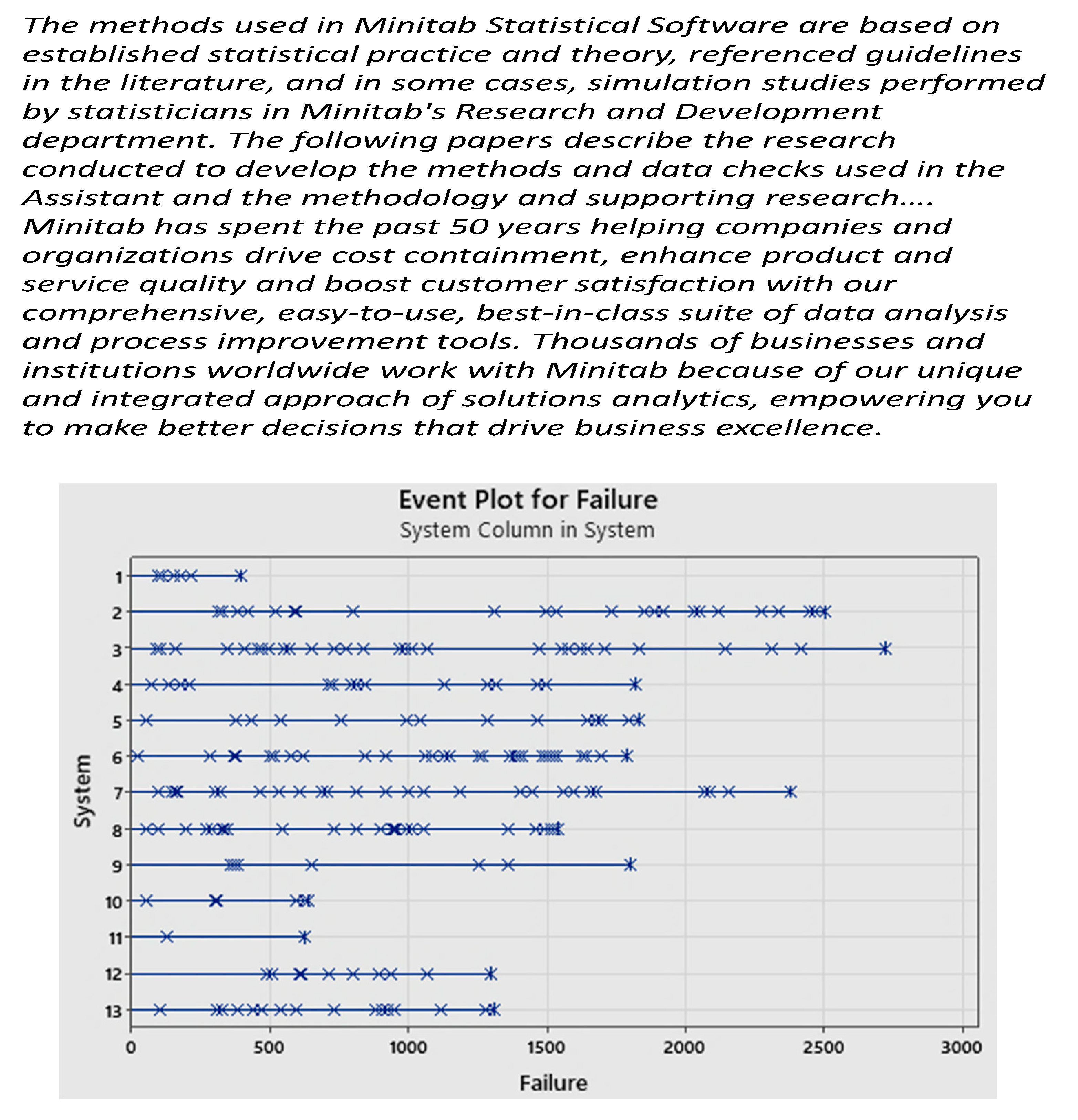
Figure 29.
Statistical Output for 13 repairable air-conditioners (Minitab 21 used).
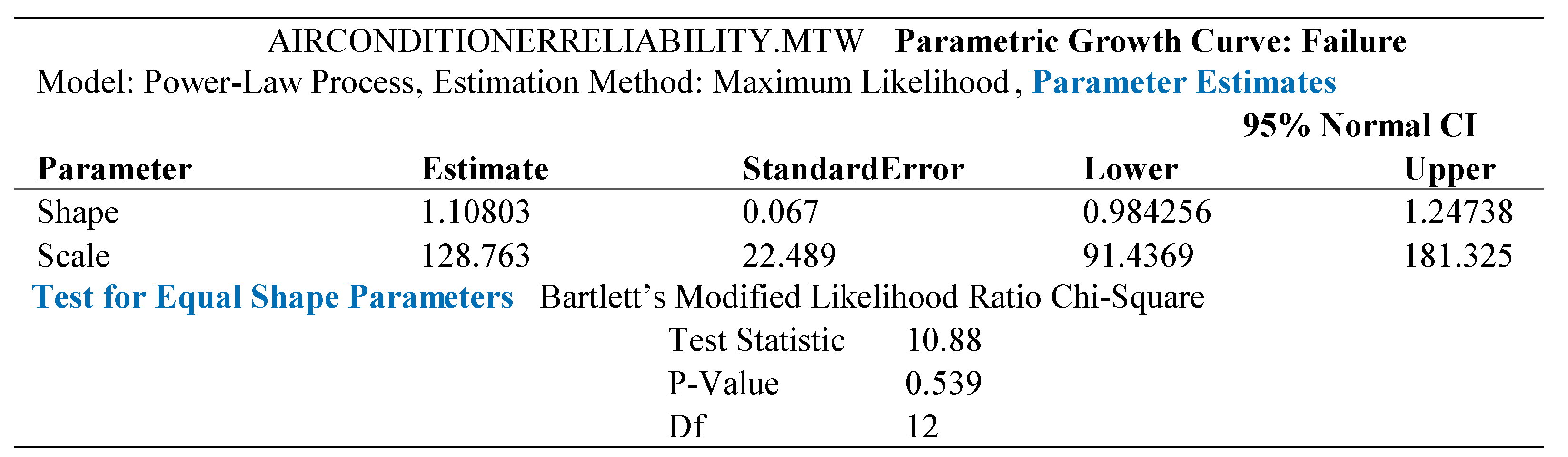
Figure 30.
Graphical Output for 13 repairable air-conditioners data (Minitab 21 used).
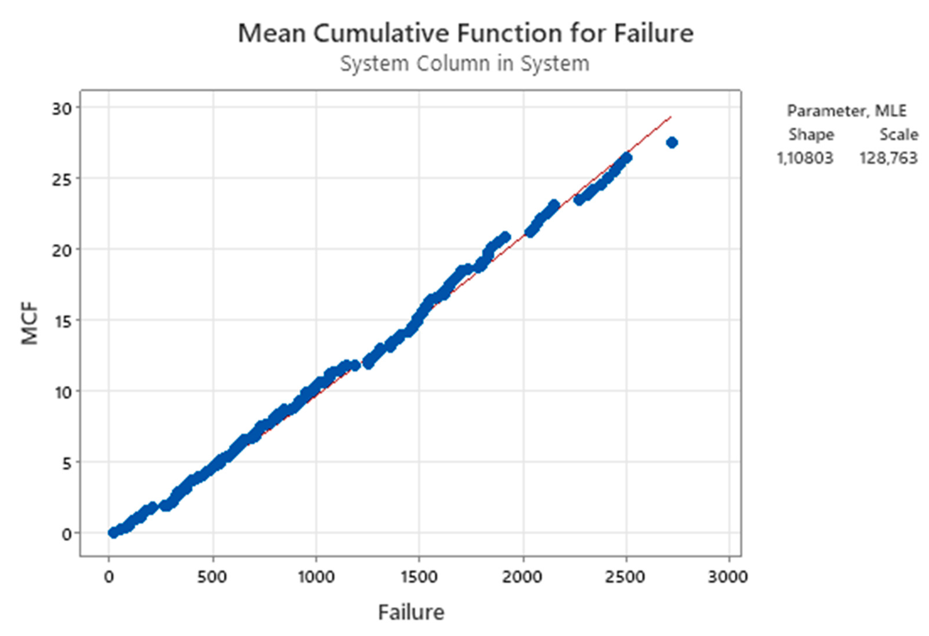
Figure 31.
Duane plot for 13 repairable air-conditioners data (Minitab 21 used).
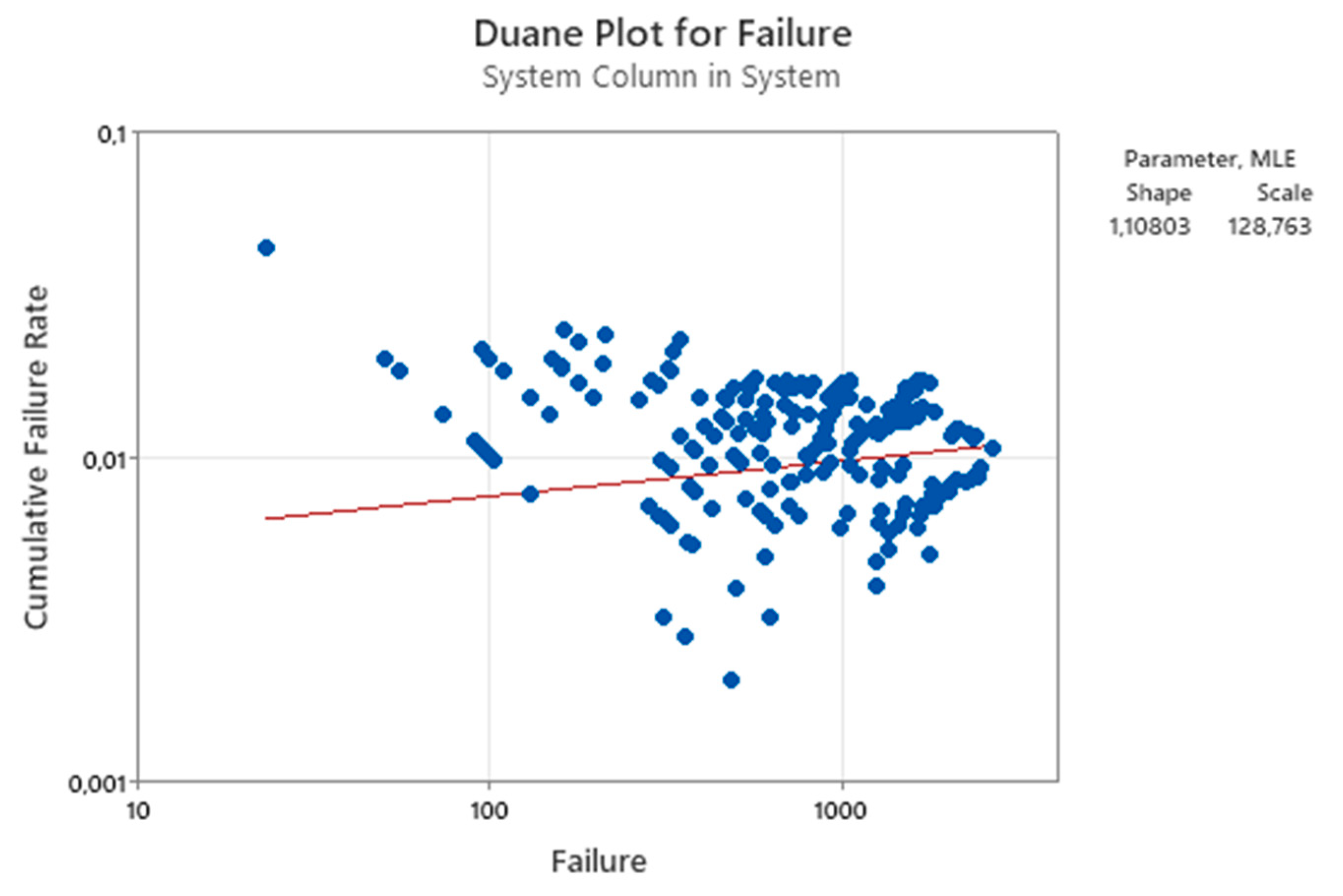
Figure 32.
Distribution of repairable air-conditioners data tij (Minitab 21 used).
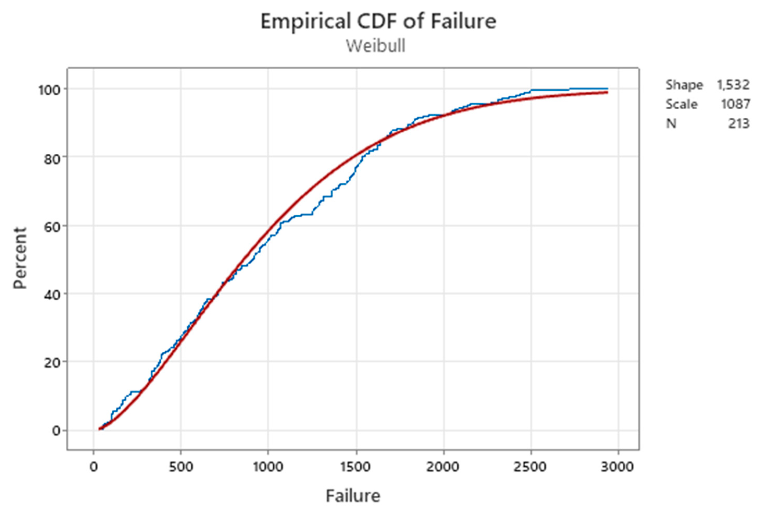
Figure 33.
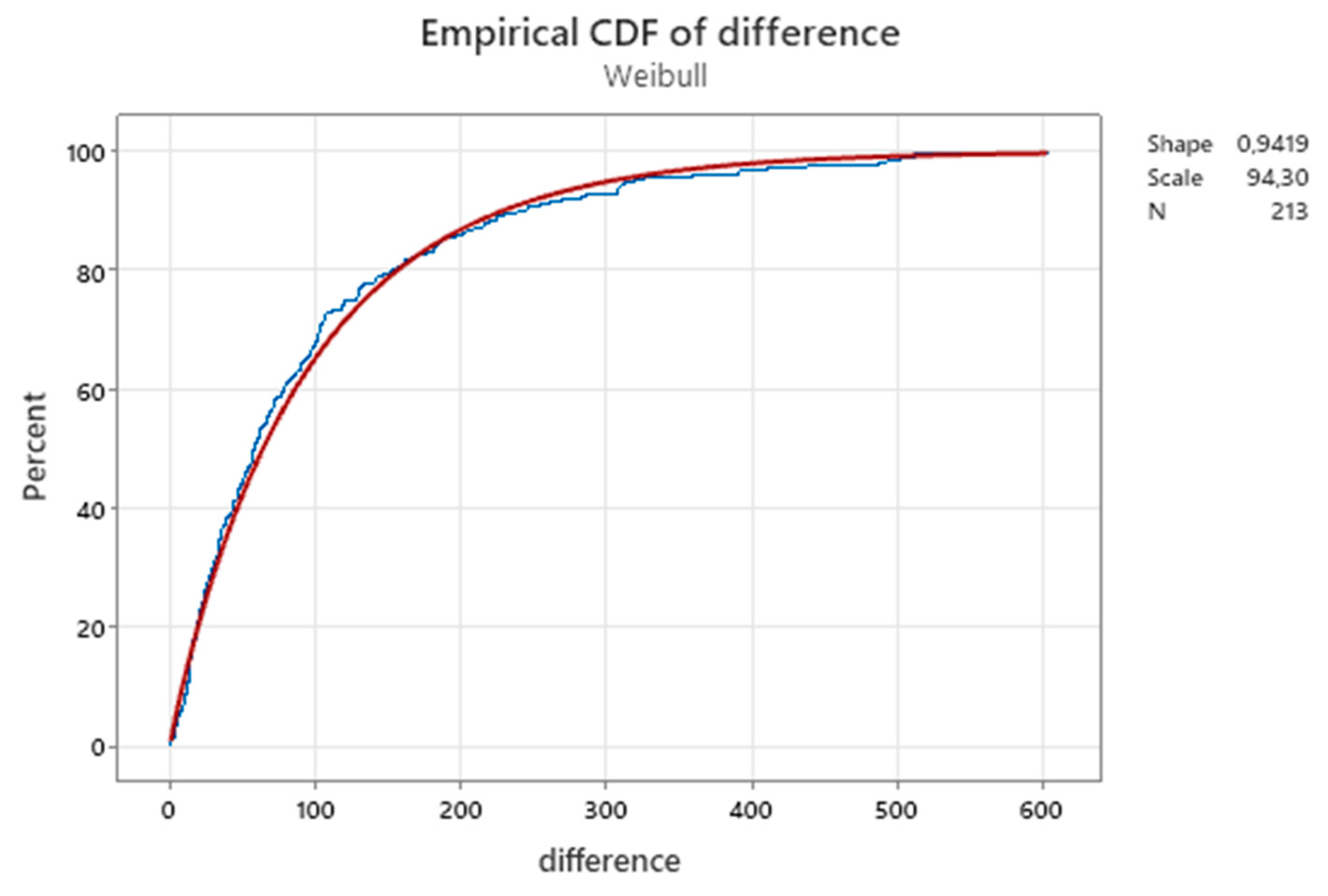
Distribution of repairable air-conditioners differences dij (Minitab 21 used).
We can compare the Figure 30 [the M(t)] with the 31 [the “cumulative failure rate”]; how it is related to “our” failure rate, as defined in our theory? Think about that ... See the figures 29, 30. The Figure 31 is the Duane Model!
The figures 32 and 33 show the distribution of times tij, and their differences dij, respectively.
From figures 30, 31, 32 we see that the shape parameter β of M(t) is estimated by Minitab as βPL=1.10803, where PL stands for “Power Law”. Notice that this estimate tells us that “there is no aging”; moreover, the figures 32 and 33 describe a completely different aging process of the air-conditioners! βW=1.532 (aging) and βd=0.9219 (no aging). Where is the TRUTH?
It is in the given Theory, RIT.
The fundamental system (integral equations) for reliability tests (duration 0-----t) [t0=0 is the start of the test and t is the end of the test], with tj times of failures is given in (10), with the kernels of Figure 28; at the end t of the reliability test, we know the empirical sampleD={t1, t2, …, tg-1, tg, t}; tg is the last failure. To estimate the parameters β and η, from the equations we compute the determinant of the integral system (in matrix form) detB(s|r) [depending on β and η]. We have, for the system (air-conditioner) 1, with failures time t1,j, and g1 failures, the formula (identical to the Likelihood)
The values maximising , for the item 1, are
and Similar results are found for all the 13, identical and repaired, air conditioners.
Same results can be found with the MLM.
Figure 34.
Transition Diagram of a repairable unit (BAO) and probability density of transitions.
From the reliability system of 13 items, we get the estimations βall and ηall of the parameters β and η:
and The CI of βall is 0.858-------1.121, with CL=95%.
Notice: βall=0.99 is slightly in the (Minitab) CI of β (0.984256-------1.24738, with CL=95%), AND the (Minitab) βPL=1.10803 is slightly in the CI of βall (0.858-------1.121, with CL=95%). The contrary would happen by choosing CL=90%!
We cannot have “enough confidence” that the (Minitab) βPL=1.10803 AND βall=0.99 are “equivalent”!
Minitab provides wrong results for repairable systems and Duane analysis: Minitab lacks scientificity and generates huge costs for Companies using them, due to their wrong analyses.
The wrong “Duane method” is based on the wrong “Duane Axiom”: "the MTBFc (the Mean Time Between Failures, instantaneous cumulated) is the ratio of the total cumulated time by the tested items, tc, to the total number of failures M(tc) experienced in the total time test interval t0-----tc". So, they write with α=0.2 ÷ 0.4, and t0 the "total time cumulated at the beginning of the total time test interval t0-----tc" where MTBF=MTBF0
For the Weibull distribution, we have h(t)=(β/η)(t/η)β-1 and (by the absurd “Duane Axiom”) MTBF=1/h(t)=t1-β ηβ/β, α=1-β with MTBF0/t01-β=constant.
The position MTBF=1/h(t) is an absolute NONSENSE, as shown before.
4. Discussion and Conclusions
Applying the G-Process we could show the way to solve various cases of practical interest: analysis of repairable systems reliability and availability, statistical estimation (and Confidence Interval evaluation) of the parameters of distributions, correct computation of Control Limits of the Control Charts, especially for Individual CC with TBE exponentially distributed and of the Douane method.
We introduced the Stochastic G-Processes which rule the relationships between the reliabilities Ri(t|s). The stochastic processes [HMP, NHMP, SMP, RP, A&RP] used for reliability analyses (to the author knowledge) are particular cases of the G-Process. We showed various cases (from papers) where errors were present due to the lack of knowledge of RIT.
The author many times tried to compel several scholars to be scientific: he did not have success (Galetto 1981-2023). Only Juran appreciated the author’s ideas when he mentioned the paper “Quality of methods for quality is important” at the plenary session of EOQC Conference, Vienna.
For the control charts, it came out that RIT proved that the T Charts, for rare events and TBE (Time Between Events), used in the software Minitab, SixPack, JMP or SAS are wrong. So doing the author increased the h-index of the mentioned authors publishing wrong papers. See Appendix A.
We suggest the readers to consider the various excerpts, especially those related to CCs: many authors have been diffusing wrong concepts for years and years…
RIT allows the scholars (managers, students, professors) to find sound methods also for the ideas shown by Wheeler in Quality Digest documents.
We proved also that Minitab software provides wrong analysis repairable systems Reliability (Minitab says “the items are aging”, while they are actually GAN after any failure).
We informed the authors and the Journals who published wrong papers by writing various letters to the Editors…: no “Corrective Action”, a basic activity for Quality. The same happened for Minitab: so, people continue taking wrong decisions…
Deficiencies in products and methods generate huge cost of DIS-quality (poor quality) as highlighted by Deming and Juran. Any book and paper are a product (providing methods). The books present financial considerations about reliability: their wrong ideas and methods generate huge cost for the Companies using them. The methods given here provide the way to avoid such costs, especially when RIT gives the right way to deal with Preventive Maintenance (risks and costs), Spare Parts Management (cost of unavailability of systems and production losses), Inventory Management, cost of wrong analyses and decisions.
We think that we provided the readers with the belief that Quality of Methods for Quality is important and with several ideas and methods to be meditated in view of the applications, generating wealth for the companies using them.
There is no “free lunch”: metanoia and study are needed and necessary.
Funding
This research received no external funding.
Conflicts of Interest
The author declares no conflicts of interest.
Abbreviations
The following abbreviations are used in this manuscript:
| LCL, UCL | Control Limits of the Control Charts (CCs) |
| L, U | Probability Limits related to a probability 1-α |
| θ | Parameter of the Exponential Distribution |
| θL-----θU | Confidence Interval of the parameter θ |
| RIT | Reliability Integral Theory |
Appendix A


There is no “free lunch”: metanoia and study are needed and necessary.
References
- Feller, W. (1967) An Introduction to Probability Theory and its Applications, Vol. 1, 3rd Ed. Wiley.
- Feller, W. (1965) An Introduction to Probability Theory and its Applications, Vol. 2, Wiley.
- Parzen, E. (1999) Stochastic Processes, Society for Industrial and Applied Mathematics.
- Papoulis, A. (1991) Probability, Random Variables and Stochastic Processes, 3rd Ed. McGraw-Hill.
- Jones, P., Smith, P. (2018) Stochastic Processes An Introduction, 3rd Ed. CRC Press.
- Knill, O. (2009) Probability Theory and Stochastic Processes with Applications, Overseas Press.
- Shannon, Weaver (1949) The Mathematical Theory of Communication, University of Illinois Press.
- Dore, P., (1962) Introduzione al Calcolo delle Probabilità e alle sue applicazioni ingegneristiche, Casa Editrice Pàtron, Bologna.
- Cramer, H., (1961) Mathematical Methods of Statistics, Princeton University Press.
- Kendall, Stuart, (1961) The advanced Theory of Statistics, Volume 2, Inference and Relationship, Hafner Publishing Company.
- Mood, Graybill, (1963) Introduction to the Theory of Statistics, 2nd ed., McGraw Hill.
- Rao, C. R., (1965) Linear Statistical Inference and its Applications, Wiley & Sons.
- Belz, M., (1973) Statistical Methods in the Process Industry, McMillan.
- Rozanov, Y., (1975) Processus Aleatoire, Editions MIR, Moscow, (traduit du russe).
- Ryan, T. P., (1989) Statistical Methods for Quality Improvement, Wiley & Sons.
- Casella, Berger, (2002) Statistical Inference, 2nd edition, Duxbury Advanced Series.
- Galetto, F., (1981, 84, 87, 94) Affidabilità Teoria e Metodi di calcolo, CLEUP editore, Padova (Italy).
- Galetto, F., (1982, 85, 94) “Affidabilità Prove di affidabilità: distribuzione incognita, distribuzione esponenziale”, CLEUP editore, Padova (Italy).
- Galetto, F., (1995/7/9) Qualità. Alcuni metodi statistici da Manager, CUSL, Torino (Italy).
- Galetto, F., (2010) Gestione Manageriale della Affidabilità”, CLUT, Torino (Italy).
- Galetto, F., (2015) Manutenzione e Affidabilità, CLUT, Torino (Italy).
- Galetto, F., (2016) Reliability and Maintenance, Scientific Methods, Practical Approach”, Vol-1, www.morebooks.de.
- Galetto, F., (2016) Reliability and Maintenance, Scientific Methods, Practical Approach”, Vol-2, www.morebooks.de.
- Deming W. E., (1986) Out of the Crisis, Cambridge University Press.
- Deming W. E., (1997) The new economics for industry, government, education, Cambridge University Press,.
- Juran, J., (1988) Quality Control Handbook, 4th ed, McGraw-Hill, New York.
- Juran, Godfrey (1998) Quality Control Handbook, 5th ed, McGraw-Hill, New York.
- Shewhart W. A., (1931) Economic Control of Quality of Manufactured Products, D. Van Nostrand Company.
- Shewhart W.A., (1936) Statistical Method from the Viewpoint of Quality Control Graduate School, Washington.
- Galetto, F., (2015) Hope for the Future: Overcoming the DEEP Ignorance on the CI (Confidence Intervals) and on the DOE (Design of Experiments, Science J. Applied Mathematics and Statistics. Vol. 3, No. 3, pp. 70-95. [CrossRef]
- D. J. Wheeler, “The normality myth”, Online available from Quality Digest.
- D. J. Wheeler, “Probability limits”, Online available from Quality Digest.
- D. J. Wheeler, “Are you sure we don’t need normally distributed data?” Online available from Quality Digest.
- D. J. Wheeler, “Phase two charts and their Probability limits”, Online available from Quality Digest.
- Galetto, F., 2019, Statistical Process Management, ELIVA press ISBN 9781636482897.
- Galetto, F., (1989) Quality of methods for quality is important, EOQC Conference, Vienna,.
- Galetto, F., (2015) Management Versus Science: Peer-Reviewers do not Know the Subject They Have to Analyse, Journal of Investment and Management. Vol. 4, No. 6, pp. 319-329. [CrossRef]
- Galetto, F., (2015) The first step to Science Innovation: Down to the Basics., Journal of Investment and Management. Vol. 4, No. 6, pp. 319-329. [CrossRef]
- Galetto F., (2021) Minitab T charts and quality decisions, Journal of Statistics and Management Systems. [CrossRef]
- Galetto, F., (2012) Six Sigma: help or hoax for Quality?, 11th Conference on TQM for HEI, Israel.
- Galetto, F., (2020) Six Sigma_Hoax against Quality_Professionals Ignorance and MINITAB WRONG T Charts, HAL Archives Ouvert, 2020.
- Galetto, F., (2021) Control Charts for TBE and Quality Decisions, submitted.
- Galetto F. (2022), “Affidabilità per la manutenzione Manutenzione per la disponibilità”, tab edezioni, Roma (Italy), ISBN 978-88-92-95-435-9, www.tabedizioni.it.
- Galetto F. (2021) ASSURE: Adopting Statistical Significance for Understanding Research and Engineering, Journal of Engineering and Applied Sciences Technology, ISSN: 2634 – 8853, 2021 SRC/JEAST-128. [CrossRef]
- Galetto F. (2023) Control Charts, Scientific Derivation of Control Limits and Average Run Length, International Journal of Latest Engineering Research and Applications (IJLERA) ISSN: 2455-7137 Volume – 08, Issue – 01, January 2023, PP – 11-45.
- Galetto, F., (1999) GIQA the Golden Integral Quality Approach: from Management of Quality to Quality of Management, Total Quality Management (TQM), Vol. 10, No. 1. [CrossRef]
- Galetto, F., (2004) Six Sigma Approach and Testing, ICEM12 –12th International Conference on Experimental Mechanics, 2004, Bari Politecnico (Italy).
- Galetto, F., (2006) Quality Education and quality papers, IPSI, Marbella (Spain).
- Galetto, F., (2006) Quality Education versus Peer Review, IPSI, Montenegro.
- Galetto, F., (2006) Does Peer Review assure Quality of papers and Education? 8th Conference on TQM for HEI, Paisley (Scotland).
- Montgomery D., (1996, 2009, 2011) Introduction to Statistical Quality Control, Wiley & Sons (wrong definition of the term "Quality", and many other drawbacks in wrong applications).
- Montgomery D., (2019) “Introduction to Statistical Quality Control”, 8th Wiley & Sons.
- Galetto, F., “Design Of Experiments and Decisions, Scientific Methods, Practical Approach”, 2016, www.morebooks.de.
- Galetto, F., “The Six Sigma HOAX versus the versus the Golden Integral Quality Approach LEGACY”, 2017, www.morebooks.de.
- Galetto, F., “Quality Education on Quality for Future Managers”, 1st Conference on TQM for HEI (Higher Education Institutions), 1998, Toulone (France).
- Galetto, F., “Quality Education for Professors teaching Quality to Future Managers”, 3rd Conference on TQM for HEI, 2000, Derby (UK).
- Galetto, F., “Quality, Bayes Methods and Control Charts”, 2nd ICME 2000 Conference, 2000, Capri (Italy).
- Galetto, F., “Looking for Quality in "quality books", 4th Conference on TQM for HEI, 2001, Mons (Belgium).
- Galetto, F., “Quality and Control Carts: Managerial assessment during Product Development and Production Process”, AT&T (Society of Automotive Engineers), 2001, Barcelona (Spain).
- Galetto, F., “Quality QFD and control charts: a managerial assessment during the product development process”, Conference ATA, 2001, Florence (Italy).
- Galetto, F., “Business excellence Quality and Control Charts”, 7th TQM Conference, 2002, Verona (Italy).
- Galetto, F., “Fuzzy Logic and Control Charts”, 3rd ICME 2002 Conference, Ischia (Italy).
- Galetto, F., “Analysis of "new" control charts for Quality assessment”, 5th Conference on TQM for HEI, 2002, Lisbon (Portugal).
- Galetto, F., “The Pentalogy, VIPSI, 2009, Belgrade (Serbia).
- Galetto, F., The Pentalogy Beyond, 9th Conference on TQM for HEI, 2010, Verona (Italy).
- Galetto, F., Papers and Documents in Academia.edu, 2015-2025.
- Galetto, F., Several Papers and Documents in the Research Gate Database, 2014.
Figure 6.
Shewhart I-CC from Brazilian Journal of Op. & Prod. Management (Figure 12 in their paper).
Figure 6.
Shewhart I-CC from Brazilian Journal of Op. & Prod. Management (Figure 12 in their paper).
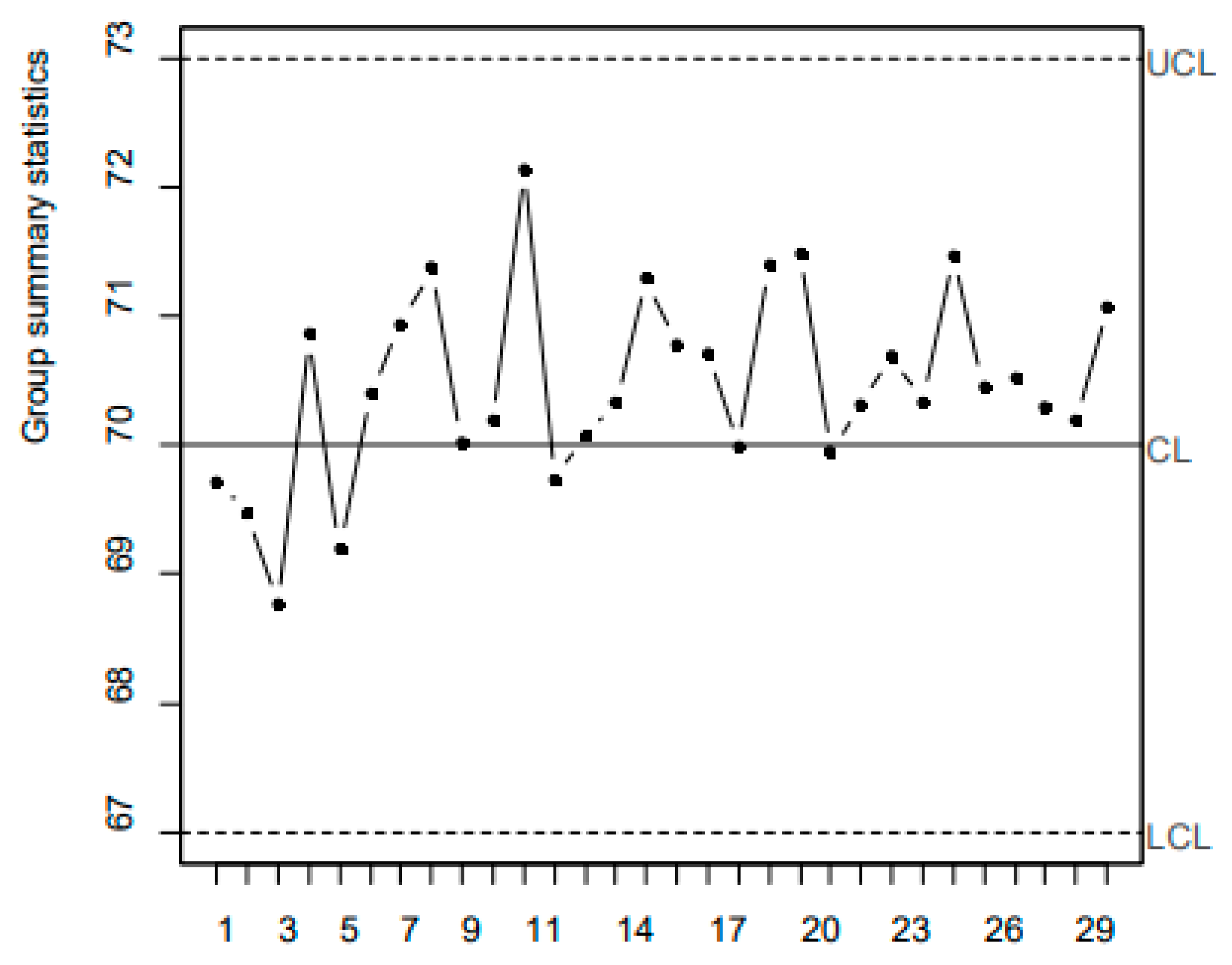
Figure 7.
Shewhart I-CC computed by F. Galetto; notice the OOC points.
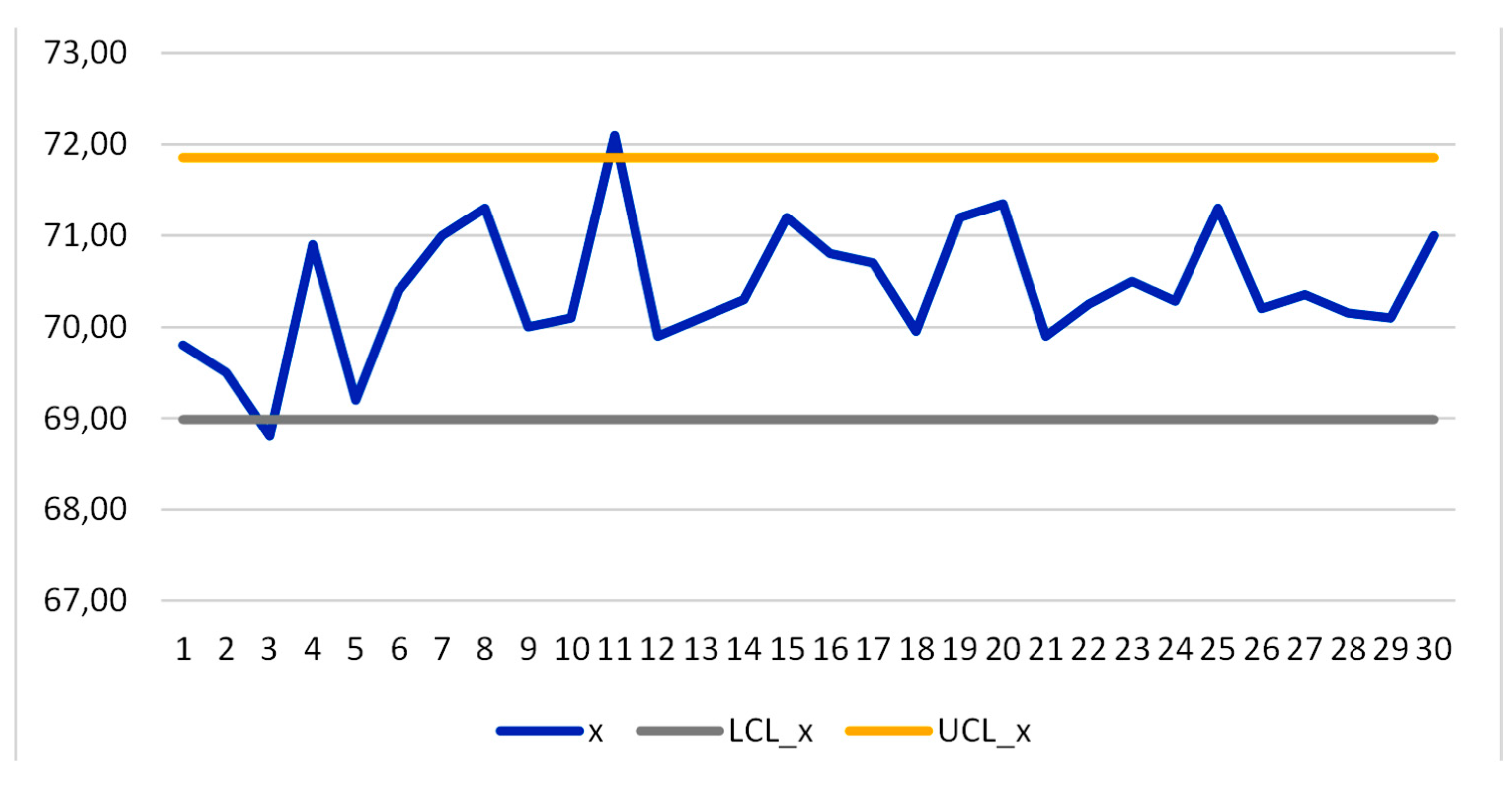
Figure 8.
The Individuals xij, the “means” of the process and the “grand mean” .
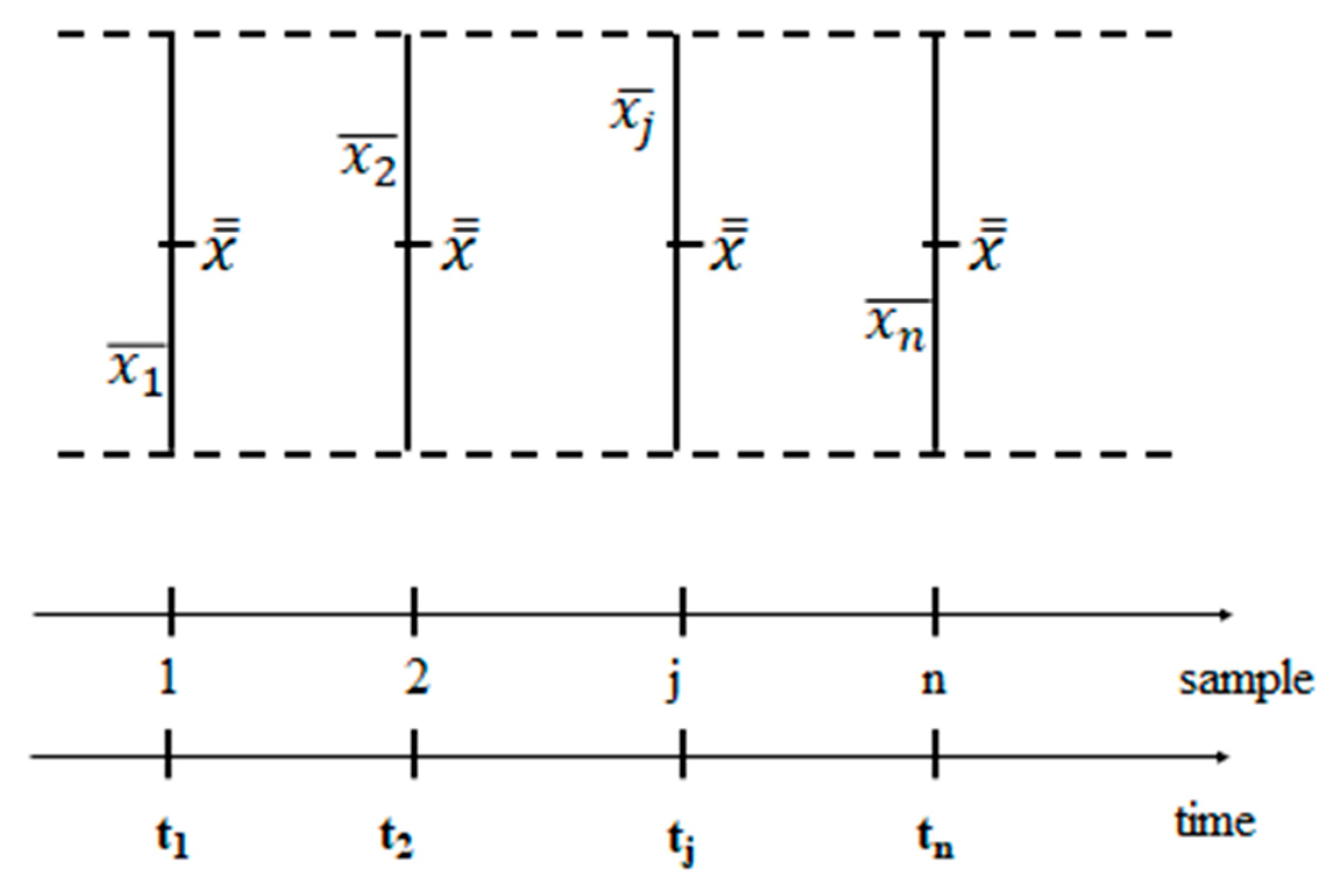
Figure 25.
CC of the Individuals (from the paper “The length-biased weighted exponentiated inverted …”), RIT used.
Figure 25.
CC of the Individuals (from the paper “The length-biased weighted exponentiated inverted …”), RIT used.
Disclaimer/Publisher’s Note: The statements, opinions and data contained in all publications are solely those of the individual author(s) and contributor(s) and not of MDPI and/or the editor(s). MDPI and/or the editor(s) disclaim responsibility for any injury to people or property resulting from any ideas, methods, instructions or products referred to in the content. |
© 2025 by the authors. Licensee MDPI, Basel, Switzerland. This article is an open access article distributed under the terms and conditions of the Creative Commons Attribution (CC BY) license (http://creativecommons.org/licenses/by/4.0/).
Copyright: This open access article is published under a Creative Commons CC BY 4.0 license, which permit the free download, distribution, and reuse, provided that the author and preprint are cited in any reuse.


