Submitted:
10 April 2025
Posted:
11 April 2025
You are already at the latest version
Abstract
Fano-resonant silicon metasurfaces exhibit extreme planar chirality, offering tremendous potential for miniaturized optical devices. However, achieving ultra-high quality factor (Q) resonance in such devices remains challenging. Here, we construct a fractal pentamer all-dielectric metasurface, of which the scale factors of second-order fractals are designed differently to introduce asymmetry. This asymmetry transforms symmetry-protected bound states in the continuum (BIC) into quasi-BIC (QBIC), achieving ultra-high Q factor Fano resonances.Magnetic dipole (MD) and transverse dipole (TD) BIC can be supported in this system, thus produce extremely narrow linewidth Fano resonances. By optimizing the asymmetric state, ultrahigh Q factor up to 4×10⁴ is reached. We numerically obtain bulk sensitivities of 1.905 μm/RIU and figures of merit (FOM) up to 5625.5. The constructed resonances are insensitive to x and y polarizations due to the specific layout of clusters proposed here. Therefore, the proposed all-dielectric metasurface demonstrates good performance in refractive index sensing, which inspires the development of new high Q factor refractive index sensors for the nondestructive identification in the far-infrared regime.
Keywords:
BIC
; dielectric metasurface
; Fano resonance
; polarization insensitivity
1. Introduction
BICs are localized states without radiation in the continuous spectra. An ideal BIC only exists in lossless infinite structures. It can be regarded as zero leakage, zero linewidth resonance, and an infinite Q factor [1,2,3,4]. And it cannot be excited directly owing to its decoupling from the radiative wave. In practice, it will be first converted into quasi-BIC with finite but still high Q factors to be excited by external sources. Due to such advantages BICs have found various applications, including beam steering [5], refractometric sensing [6,7,8,9], chiral enhancement [10,11,12], non-linear harmonic generation [13,14,15], field enhancement , photodetection [16,17,18] and imaging [19,20,21,22], since its experimental demonstration[23,24,25].
Based on the physical mechanisms of formation, BICs can be generally classified into three types of which the most direct type is the symmetry-protected BIC. The electromagnetic energy in symmetry-protected BIC cannot couple outward because the spatial symmetry of a mode does not match the spatial symmetry of radiation[1]. Since symmetry-protected BIC can be excited at the point of Brillouin zone in periodic structures with symmetries, metasurfaces which is composed of periodic unit cells artificially are used to construct symmetry-protected BIC[23]. By breaking the symmetry in various ways, they can be transformed into QBICs with high Q factors. To achieve this transformation, excitation field symmetry or the structure symmetry should be broken. The symmetry of excitation is usually broken through oblique incidences [23,26]. And the common method of breaking structural symmetry is deforming the unit of metasurface to break in-plane symmetry [27,28,29,30,31]. Thus, symmetry-protected BICs can be constructed and transformed into QBICs within metasurfaces.
In sensing applications, high Q factor are desirable performance goals. Initially, benefiting from the development of surface plasmon theory, various kinds of metal-based metasurface sensors finds widely application due to their high field concentration [32,33,34,35,36]. For instance, in [32], by adjusting the gap between two metallic resonant rings, a quasi-BIC resonance with a Q factor of approximately 143 is achieved in the terahertz range. However, the above works based on metallic metasurface inevitably suffer from significant ohmic loss problem especially at ultra-high frequency, which severely degrade the Q factor. To solve this problem, all-dielectric metasurfaces are used to sensing due to their lower intrinsic losses. These resonators with high Q factors have extremely narrow resonance linewidth, enabling detection of small frequency shifts caused by subtle changes. All-dielectric metasurfaces are usually composed of structured high index dielectric materials, thus fano resonance with high Q can be supported. Fano resonance is asymmetric spectral profile produced by the destructive interference of continuous states and discrete localized states. Fano resonances in metaurfaces are usually realized through symmetry breaking and can be described in terms of interactions between bright and dark modes. The bright mode is excited by the incident light and is highly radiative, while the dark mode is subradiant and is only accessible through the near field excitation by the bright mode[37].Recently, Fano resonances of metasurfaces have been linked to BIC. The frequency dependence of the transmission is described rigorously by the Fano formula, and the Fano parameters are expressed explicitly through the material and geometrical parameters of the metasurface. Fano parameter becomes ill-defined for a true BIC thus corresponding to a collapse of the Fano resonance when any features in the transmission spectra disappear, and the resonant mode is transformed into dark mode, which does not manifest itself in scattering spectra.[27]. In metasurfaces, the Fano lineshape can be optimised by decreasing the structural asymmetry of the unit to give a sharp spectral response. Its sharp spectral characteristic can provide high Q, meanwhile, its significant near-field enhancement can supply high sensitivity.
In the last few years, many all-dielectric metasurface sensors have been demonstrated for optical sensing [8,38,39,40,41,42,43,44,45,46]. For example, in [39], dual-band symmetry-protected BICs are proposed based on the hybridization of surface lattice resonances (SLR) in periodic silicon bipartite nanodisk arrays of which the in-plane structural symmetry is broken by displacing the central nanodisk from the center of the unit cell. The hybridization of Mie SLRs results in dual-band electric quadrupole (EQ) and MD BICs. The spectral separation and the quality factors of these two quasi-BICs can be conveniently tuned by varying the nanodisk diameter or the lattice period. Its highest Q factor can reach 1240 and FOM can reach 1200. In [41], the unit is composed of a pair rotated rectangular silicon nanobar. The excited quasi-BIC mode exhibits a dominant TD and EQ resonant property with a strong near-field confined at the surface of nanobar width, indicating strong interaction between the incident light and samples. Such design results in a near-infrared sensor with a Q factor of 2500, and sensitivity of 612 nm/RIU. In[8], the all-dielectric metasurface based on asymmetric silicon square tetramer is designed. Such metasurface can induce TD and MD resonances which produce multi-extremely narrow linewidth Fano resonances governed by QBIC. It get maximum sensitivity reaches up to 1.43 m/RIU and Q factor up to . These studies utilized all-dielectric metasurfaces to obtain sensors with relatively high Q factors and FOMs.
In this work, we proposed ultra-high Q resonance at far infrared frequencies driven by BIC in all-dielectric metasurface structure with a periodic array of asymmetric second-order fractal clusters. By tuning the second-order fractal factor, in-plane symmetry of the unit cell is broken. Three sharp Fano resonance with modulation depths approaching 100% can be achieved by adjusting the structural dimensions and asymmetry parameter. By controlling the asymmetric parameter , the resonance reach a maximum Q factor of . Cartesian multipole decomposition and electric field distribution show that three resonances mainly arise from MD1, MD2 and TD respectively. Besides, the polarization dependence of this metasurface is studied. Finally, the refractive index sensitivity analysis of the proposed sensor demonstrates the highest sensitivity of 1.905m/RIU and a FOM of 5625.5. The designed sensor provides a method for refractive indices sensing for liquid samples in the far-infrared range.
2. Materials and Methods
The schematic diagram of the proposed asymmetric metasurface is depicted in Figure 1. The metasurface unit consists of a second-order fractal silicon nanodisk (refractive index ) arranged on a Potassium Bromide (KBr) substrate (refractive index ). Si and KBr are chosen as the materials for the dielectric nanodisk and substrate respectively because their losses can be neglected in the operating wavelength range of this sensor. The refractive indexes and losses of Si and KBr are obtained from Palik [47].
The geometric parameters of the unit cell are presented in Fig .Figure 1(A) and (B). Here, the period is , the height of nanodisk is 4.25m and the height of substrate is 0.5m. The fundamental structure is a square with side length of . In first-order fractal iteration, small squares with a side length of are removed from the center of each side, where is the first-order scaling factor. This iteration rule is then applied to each side of the first-order fractal to obtain the second-order fractal. This fractal structure can be infinitely repeated to obtain increasingly complex self-similar structures.
As shown in Figure 1B, when performing the second-order fractal, the squares in the northeast and southwest corners are with the scaling factor , while the other two squares are with factor . When , the unit is symmetric in the x-y plane. When , in-plane symmetry breaking is introduced. The difference between and is denoted as . We simulate the proposed metasurface structure using the finite element method. The x and y directions are set with periodic boundary conditions. The excitation source is a x-polarized plane wave propagating along the -z direction.
3. Results and Discussion
3.1. Transmission Spectra and Field
We analyze the the transmission spectra under different fractal factor difference while keeping constant during simulation. The results are shown in Figure 2. Firstly, for (symmetric structure), there is only one Fano resonance peak at 17.21 m. As increases, the in-plane symmetry is broken, the BIC energy can be radiated outside, leading to transition between BIC mode and the continuum free space, which produce additional Fano resonance. Thus, two extra resonances appear in the transmission spectra. Among the three resonances, we refer the one with the longest wavelength as mode3, the one with the shortest wavelength as mode1, and the rest as mode2. It can be observed that mode3 has ultra-narrow resonance, indicating ultrahigh Q factor. Mode1 and mode2 have wider resonance linewidths, suggesting that the symmetry breaking increases the radiative channels at the resonance, resulting in more energy leakage and corresponding decrease in the Q factor. Additionally, as increases, the asymmetry of metasurface increases, leading to increasing linewidths of the three resonances, accompanied by a blue shift in the resonance wavelength. Besides, the distance between mode1 and mode2 also becomes significantly larger. For mode3, the asymmetry caused by the difference of fractal scale factors at diagonal positions compensates for the spatial symmetry mismatch between the BIC mode and the incident excitation. A radiative channel is formed between the metasurface and free space, allowing the BIC energy to radiate outside, thus transforming the BIC mode into a quasi-BIC mode with high Q factor and finite linewidth. The smaller the symmetry breaking is, the narrower the radiative channel is, resulting in higher Q factor. However, when becomes too small, the linewidth of resonance is extremely narrow, but its modulation depth is also low, resulting in difficulty in sensing applications under the case that there is external interference. On the other hand, when is large, the linewidth of resonance increases rapidly resulting in lower Q factor. To make a trade-off, we choose as the operating parameter for this sensor.
According to the simulation results, all three resonances are of Fano resonance profile. To calculate Q factor of the fano resonances, we fit transmission spectra with Fano model by using the classical Fano formulation (1) [48,49].
where represents the resonant angular frequency, is the resonance linewidth, refers to transmission offset, means the continuum-discrete coupling constant, and q is the Fano parameter determining the asymmetry of the resonance profile.
Figure 3 shows the fitted results under . It can be observed that the fitted results match the simulated curve closely. The fitted parameters of mode 3 are , , , and . Then the resonant Q factor of mode3 is calculated as 40793 by . Similarly, fitted results of mode1 and 2 show the linewidths of 35.48 and 58.50, Q factors of 2054.2 and 3112.9 respectively. Therefore, it can be concluded that the resonance linewidth of mode3 is significantly smaller than the others, resulting in the highest Q factor. Thus, mode3 is chosen as the main operating mode for the sensor proposed.
We further investigate the relationship between the Q factor of mode3 and the asymmetric parameter , which is defined here as the ratio of area difference () between original second-order fractal square and its symmetrically broken square to area (S) of original second-order fractal square.
where and are shown in Figure 1.
Based on previous studies [27], the Q factor of the symmetry-protected quasi-BIC exhibits an inverse quadratic law with the asymmetric parameter of metasurface ().
In similar way, we calculate Q factors for a serious different asymmetric parameters =0.0416, 0.0654, 0.091, 0.12, 0.151, 0.185, 0.223, 0.265, 0.312 and 0.422. The results is shown in Figure 4. As approaches zero, the resonant Q factor tends to infinity. The relationship between Q factor of mode3 and the asymmetric parameter follows the inverse quadratic law. It indicates that the resonance of mode3 is excited by the symmetry-protected quasi-BIC resulting from the symmetry breaking.
To further investigate the physical mechanism of all resonances under symmetric and symmetric broken cases, the electric and magnetic fields of the metasurface at the resonance wavelength are calculated and shown in Figure 5(A) to Figure 5(L). Figure 5(A), Figure 5(E) and Figure 5(I) are the electric and magnetic fields under symmetric case. As shown in the figures, the electric field vector forms annular distribution surrounding the axis of the dielectric nanodisk along y, which generates a magnetic moment in y direction. MD mode is excited. Under asymmetric cases, the fields at the three resonances are shown in the Figure 5(B), Figure 5(F), Figure 5(J), Figure 5(C), Figure 5(G), Figure 5(K) and Figure 5(D), Figure 5(H), Figure 5(L). The electric field vectors of mode1 (Figure 5(F)) and mode2 (Figure 5(G)) still exhibit annular distribution, indicating MD mode resonances. However, unlike that in symmetric case under which the axis of annular electric field is along y. The axis of annular electric field for mode1 (Figure 5(B)) is rotated 45 degrees clockwise from y axis (Figure 5(A)). Similarly, axis of annular electric field of mode2 is approximately orthogonal to mode1 (Figure 5(C)), rotating 45 degrees counterclockwise from y axis. Besides, as is shown in Figure 5(A), Figure 5(B) and Figure 5(C), the electric field intensity for three resonances above is confined in the left and right gaps of the unit cell in the horizontal direction. While Figure 5(E), Figure 5(F) and Figure 5(G) show the electric field intensity concentrates at the upper and lower ends of the nanodisks in z direction. Such concentrated field distribution provides higher sensitivity for the sensor proposed. According to their annular distribution feature of electric field vector, all the three resonances above are MD mode resonance. Therefore, when symmetry is broken, the original single resonance under symmetric case is transformed into two resonances as shown in Figure 2.
However, Figure 5(D), Figure 5(H) and Figure 5(L) shows the electric and magnetic field of mode3. In this case, the electric field vectors form two adjacent loops which rotates in opposite directions in y-z plane (Figure 5(H)), which develop two magnetic moments along x axis, but in opposite direction. Consequently, they provide an annular magnetic field in x-z plane (Figure 5(L)). Such magnetic field can be effectively represented as magnetic dipoles arranged end-to-end along the circumference of the loop, resulting in a TD moment in y direction. Therefore, mode3 resonance is different from MD resonances discussed above since it is excited by TD. Besides, the magnetic field enhancement is much lager than that of other modes. Thus, it can suppress radiation loss effectively, resulting in a large Q factor. Besides, Figure 5(D) shows the electric field intensity of mode3 is confined in the up and down gaps of the unit cell in the horizontal direction. While electric field intensity concentrates at the middle of the nanodisks in z direction as shown in Figure 5(H). Such concentrated field distribution provides higher sensitivity for the sensor proposed.
3.2. Multipole Decomposition
In order to further understand the properties of each resonance, we use multipole decomposition in the Cartesian coordinate system for quantitative analysis. Firstly, we extract the displacement current density based on the electric field . Here, represents the relative permittivity at the position vector r. By integrating the current density within the dielectric, we can calculate the multipole moments. Then, we calculate the far-field scattering power spectra of each multipole moment. By summing up scattering powers of all multipole moments, we obtain the total scattering power spectra. For this metasurface, higher order multipole moments can be ignored, so we calculate eight types of multipole moments as follows: , , , , , , and , which represent electric dipole, magnetic dipole, toroidal dipole, electric quadrupole, magnetic quadrupole, toroidal quadrupole, electric octupole, and magnetic octupole. The formulas for calculating each multipole moment are as follows[50,51]
Here, r represents the position vector, c is the speed of light, refers to the angular frequency, and represent the x, y, z directions respectively. For the quadrupole and octupole moments, a simplified notation is used. For example, indicates that the second term (right side of the arrow) is obtained by interchanging the subscripts and in the first term (left side of the arrow) while keeping unchanged.The far-field scattered power of the multipole moment can be calculated as[51]
The results of the multipole decomposition are shown in Figure 6. It can be observed that the dominant multipole mode contributing to mode3 is the TD, with a subsequent contribution from the magnetic quadrupole. On the other hand, the dominant multipole mode contributing to mode1, mode2 and symmetric mode is MD, with a subsequent contribution from the electric quadrupole. These results are consistent with the electric and magnetic field distributions presented in Figure 5.
3.3. Polarization and Dimension Influence
To analyze the performance of the designed metasurface under different liner polarization, the transmitted spectra for x and y polarizations are shown in Figure 7. The dashed line is the case of x-polarized wave incidence, while the solid line represents the case of y-polarized wave incidence. From the results, it can be observed that the two MD resonances and one TD resonance can be excited under both polarization. Besides, there is almost no difference in their modulation depth and resonance wavelengths. It indicates that the obtained resonances are insensitive to x and y polarization.
To analyze the influence of geometric parameters on transmission spectra, we calculate the transmission spectra for various thickness of substrate m=0.4m, 0.6m, 0.8m, various height of nanodisk h=4m, 4.25m, 4.5m and various period P=9.75m, 10m, 10.25m. The corresponding results are shown in Figure 8(A), Figure 8(B) and Figure 8(C) respectively. We set fractal factor difference =0.04, and other geometric parameters the same as the parameters used in Figure 1 except the variable geometric parameter.
It can be seen that as the height of dielectric nanodisk h and the thickness of substrate m increase, all three resonances have a redshift, while the resonance linewidth remains relatively unchanged. Among them, mode 3 exhibits a larger variation in resonance wavelength when changing m, while modes 1 and 2 show a larger variation when changing h. Generally, h has a more significant effect on the resonance wavelength. When period P increases, all three resonances have a blueshift. Furthermore, the resonance linewidth of mode 3 varies less than mode1 and mode2 versus P. Linewidth is the least at period P=10m. In conclusion, compared with linewidth, resonant wavelength of these three resonances is more sensitive to geometric parameters. Besides, the linewidth of mode 3 changes less than mode1 and mode2. The modulation depth of these three resonances keeps stable. Since only wavelength varies significantly with geometric parameters for resonance of mode 3, it provides possibility for adjusting resonance wavelength by manipulating geometric parameters.
3.4. Refractive Index Sensing
The all-dielectric metasurface sensor proposed based on second-order fractal can excite high Q Fano resonances. Thus, it is well suited to detecting minimal wavelength shift which can be used to measure refractive index of liquid.
Firstly, we studied the relationship between the sensor’s wavelength shift caused by microliquid sample and its height. We calculate wavelength shift by assuming that the gaps among silicon nanodisk are filled with water (refractive index ). The variation of wavelength shift versus the height of water sample is achieved in Figure 9. As the height of water sample increases from 0m (unloaded) to 4.25m, redshift of mode3 occurs. Wavelength shift increases slowly when the height of sample is less than 1 m and increases quickly between sample height of 1m and 3.5m. Then, tends to a constant when the sample height is larger than 3.5m, which is close to the height of silicon nanodisk. Such characteristic can be attributed to the distribution of electric field intensity of mode 3 in z direction (Figure 5(H)). Wavelength shift increases quickest at middle range of nanodisk height where electric field has greatest concentration. Similarly, when the height of sample is near to the top of nanodisk (4.25m), the wavelength shift becomes much smaller. Thus, the height of sample should be close to top range of nanodisk so that influence of sample height on refractive index measurement can be ignored.
To investigate sensing performance of the sensor proposed, we choose five different liquid samples with refractive indices ranging from 1.333 to 1.489 and develop simulation model to retrieve the refractive index. According to discussion above, the height of liquid samples are set to the same as height of nanodisk of 4.25m to avoid influence of sample height on refractive index results. The liquid samples chosen have refractive indices n as follows: water sample with , ethanol sample () with , pentanol sample () with , carbon tetrachloride sample () with , and benzene sample () with . We compare sensitivity for the three resonance modes. Transmission spectra loaded with different liquid samples are shown in Figure 10(A) (for mode3) and Figure 10(B) (for mode1 and mode2). The results indicate that the larger the refractive index of the liquid sample is, the larger the resonance wavelength shift is for all the three resonances. Here, the refractive index sensitivity () is defined as the resonance wavelength shift caused by a unit change in refractive index, i.e . Besides, to quantitatively describe the sensing performance of the sensor, we define FOM=·/2c=, which concerns sensitivity, Q factor and resonance wavelength. where is the resonant wavelength, linewidth is obtained by fitting the transmission spectra loaded with liquid sample using equation (1).For each resonance mode, average linewidths at five refractive indices are used to calculate FOM.
Figure 10(C) shows linear fitting results on resonance wavelength shift versus corresponding refractive index. Based on that, refractive index sensitivity and FOM results for the three modes are listed in Table 1. It shows that mode3 has the highest FOM among the three modes.
Ultimately, We compare the performance of presented metasurface sensor with some other sensors in Table 2. It shows that our sensor has a great sensing performance.
4. Conclusions
A fractal all-dielectric metasurface sensor proposed here can generate TD quasi-BIC resonance, which perform high Q factor. By manipulating the second-order fractal scale factor of fractal structure, spatially symmetry is broken and high Q quasi-BIC resonance can be excited. Multipole decomposition and near-field distribution confirm the dominant role of the TD response. Such TD resonance exhibits typical symmetrically protected BIC characteristics, achieving a Q factor of approximately by controlling the asymmetric parameter. Additionally, this structure exhibits nearly identical transmission spectra for x and y-polarized incident planewaves, meeting the polarization-insensitive requirements in practical applications. Simulation results for refractive index sensing of five different liquid samples demonstrate a refractive index sensitivity of approximately 1.789 m/RIU and an FOM of 5625.5, indicating superior performance of the sensor. Our all-dielectric metasurface sensor exhibits high Q resonances, enabling detection of tiny wavelength shift. Thus, it holds great potential for non-destructive sensing and detection applications across various fields.
Author Contributions
Conceptualization, H.S. and H.D.; methodology, H.S. and H.D.; software, H.S. and H.D.; validation, H.S. and J.Z.; formal analysis, J.Z. and T.X.; investigation, H.S., H.D. and J.Z.; resources, X.W.; data curation, J.Z. and T.X.; writing—original draft preparation, H.S.; writing—review and editing, J.Z.; visualization, T.X.; supervision, X.W.; project administration, X.W. All authors have read and agreed to the published version of the manuscript.
Funding
This research received no external funding.
Data Availability Statement
The original contributions presented in this study are included in the article. Further inquiries can be directed to the corresponding author.
Conflicts of Interest
The authors declare no conflict of interest.
References
- Hsu, C.W.; Zhen, B.; Stone, A.D.; Joannopoulos, J.D.; Soljačić, M. Bound states in the continuum. Nature Reviews Materials 2016, 1, 1–13. [Google Scholar] [CrossRef]
- Koshelev, K.; Bogdanov, A.; Kivshar, Y. Meta-optics and bound states in the continuum. Science Bulletin 2019, 64, 836–842. [Google Scholar] [CrossRef] [PubMed]
- Azzam, S.I.; Kildishev, A.V. Photonic bound states in the continuum: from basics to applications. Advanced Optical Materials 2021, 9, 2001469. [Google Scholar] [CrossRef]
- Joseph, S.; Pandey, S.; Sarkar, S.; Joseph, J. Bound states in the continuum in resonant nanostructures: an overview of engineered materials for tailored applications. Nanophotonics 2021, 10, 4175–4207. [Google Scholar] [CrossRef]
- Qin, H.; Chen, S.; Zhang, W.; Zhang, H.; Pan, R.; Li, J.; Shi, L.; Zi, J.; Zhang, X.D. Optical moiré bound states in the continuum. Nature Communications 2024, 15. [Google Scholar] [CrossRef]
- Mesli, S.; Yala, H.; Hamidi, M.; BelKhir, A.; Baida, F.I. High performance for refractive index sensors via symmetry-protected guided mode resonance. Optics Express 2021, 29, 21199–21211. [Google Scholar] [CrossRef]
- Gao, J.Y.; Liu, J.; Yang, H.; Liu, H.; Zeng, G.; Huang, B. Anisotropic medium sensing controlled by bound states in the continuum in polarization-independent metasurfaces. Optics express 2023, 31 26, 44703–44719. [Google Scholar] [CrossRef]
- Chen, X.; Zhang, Y.; Cai, G.; Zhuo, J.; Lai, K.; Ye, L. All-dielectric metasurfaces with high Q-factor Fano resonances enabling multi-scenario sensing. Nanophotonics 2022, 11, 4537–4549. [Google Scholar] [CrossRef]
- Ndao, A.; Hsu, L.; Cai, W.; Ha, J.; Park, J.; Contractor, R.; Lo, Y.; Kanté, B. Differentiating and quantifying exosome secretion from a single cell using quasi-bound states in the continuum. Nanophotonics 2020, 9, 1081–1086. [Google Scholar] [CrossRef]
- Droulias, S. Chiral sensing with achiral isotropic metasurfaces. Physical Review B 2020, 102, 075119. [Google Scholar] [CrossRef]
- Deng, Q.; Li, X.; Hu, M.; et al. Advances on broadband and resonant chiral metasurfaces. npj Nanophoton 2024, 1, 20. [Google Scholar] [CrossRef]
- Tanaka, K.; Arslan, D.; Fasold, S.; Steinert, M.; Sautter, J.; Falkner, M.; Pertsch, T.; Decker, M.; Staude, I. Chiral bilayer all-dielectric metasurfaces. ACS nano 2020, 14, 15926–15935. [Google Scholar] [CrossRef] [PubMed]
- Koshelev, K.L.; Tonkaev, P.; Kivshar, Y.S. Nonlinear chiral metaphotonics: a perspective. Advanced Photonics 2023, 5, 064001. [Google Scholar] [CrossRef]
- Liu, Z.; Xu, Y.; Lin, Y.; Xiang, J.; Feng, T.; Cao, Q.; Li, J.; Lan, S.; Liu, J. High-Q quasibound states in the continuum for nonlinear metasurfaces. Physical review letters 2019, 123, 253901. [Google Scholar] [CrossRef]
- Koshelev, K.; Tang, Y.; Hu, Z.; Kravchenko, I.I.; Li, G.; Kivshar, Y. Resonant Chiral Effects in Nonlinear Dielectric Metasurfaces. ACS Photonics 2023, 10, 298–306. [Google Scholar] [CrossRef]
- Wang, W.; Besteiro, L.V.; Yu, P.; Lin, F.; Govorov, A.O.; Xu, H.; Wang, Z. Plasmonic hot-electron photodetection with quasi-bound states in the continuum and guided resonances. Nanophotonics 2021, 10, 1911–1921. [Google Scholar] [CrossRef]
- Wang, Y.; Yu, Z.; Zhang, Z.; Sun, B.; Tong, Y.; Xu, J.B.; Sun, X.; Tsang, H.K. Bound-states-in-continuum hybrid integration of 2D platinum diselenide on silicon nitride for high-speed photodetectors. ACS Photonics 2020, 7, 2643–2649. [Google Scholar] [CrossRef]
- Gao, X.D.; Fei, G.T.; Xu, S.H.; Zhong, B.N.; Ouyang, H.M.; Li, X.H.; Zhang, L.D. Porous Ag/TiO2-Schottky-diode based plasmonic hot-electron photodetector with high detectivity and fast response. Nanophotonics 2019, 8, 1247–1254. [Google Scholar] [CrossRef]
- Seo, I.C.; Kim, S.; Woo, B.H.; Chung, I.S.; Jun, Y.C. Fourier-plane investigation of plasmonic bound states in the continuum and molecular emission coupling. Nanophotonics 2020, 9, 4565–4577. [Google Scholar] [CrossRef]
- Zhou, C.; Qu, X.; Xiao, S.; Fan, M. Imaging Through a Fano-Resonant Dielectric Metasurface Governed by Quasi–bound States in the Continuum. Physical Review Applied 2020, 14, 044009. [Google Scholar] [CrossRef]
- Romano, S.; Mangini, M.; Penzo, E.; Cabrini, S.; De Luca, A.C.; Rendina, I.; Mocella, V.; Zito, G. Ultrasensitive surface refractive index imaging based on quasi-bound states in the continuum. ACS nano 2020, 14, 15417–15427. [Google Scholar] [CrossRef] [PubMed]
- Siefke, T.; Hurtado, C.B.R.; Dickmann, J.; Dickmann, W.; Käseberg, T.; Meyer, J.; Burger, S.; Zeitner, U.; Bodermann, B.; Kroker, S. Quasi-bound states in the continuum for deep subwavelength structural information retrieval for DUV nano-optical polarizers. Optics Express 2020, 28, 23122–23132. [Google Scholar] [CrossRef] [PubMed]
- Hsu, C.W.; Zhen, B.; Lee, J.; Chua, S.L.; Johnson, S.G.; Joannopoulos, J.D.; Soljačić, M. Observation of trapped light within the radiation continuum. Nature 2013, 499, 188–191. [Google Scholar] [CrossRef] [PubMed]
- Plotnik, Y.; Peleg, O.; Dreisow, F.; Heinrich, M.; Nolte, S.; Szameit, A.; Segev, M. Experimental observation of optical bound states in the continuum. Physical review letters 2011, 107, 183901. [Google Scholar] [CrossRef]
- Gansch, R.; Kalchmair, S.; Genevet, P.; Zederbauer, T.; Detz, H.; Andrews, A.M.; Schrenk, W.; Capasso, F.; Lončar, M.; Strasser, G. Measurement of bound states in the continuum by a detector embedded in a photonic crystal. Light: Science & Applications 2016, 5, e16147–e16147. [Google Scholar]
- Fan, K.; Shadrivov, I.V.; Padilla, W.J. Dynamic bound states in the continuum. Optica 2019, 6, 169–173. [Google Scholar] [CrossRef]
- Koshelev, K.; Lepeshov, S.; Liu, M.; Bogdanov, A.; Kivshar, Y. Asymmetric metasurfaces with high-Q resonances governed by bound states in the continuum. Physical review letters 2018, 121, 193903. [Google Scholar] [CrossRef]
- Li, S.; Zhou, C.; Liu, T.; Xiao, S. Symmetry-protected bound states in the continuum supported by all-dielectric metasurfaces. Physical Review A 2019, 100, 063803. [Google Scholar] [CrossRef]
- Han, S.; Pitchappa, P.; Wang, W.; Srivastava, Y.K.; Rybin, M.V.; Singh, R. Extended bound states in the continuum with symmetry-Broken terahertz dielectric metasurfaces. Advanced Optical Materials 2021, 9, 2002001. [Google Scholar] [CrossRef]
- Li, Z.; Zhou, L.; Liu, Z.; Panmai, M.; Li, S.; Liu, J.; Lan, S. Modifying the Quality Factors of the Bound States in the Continuum in a Dielectric Metasurface by Mode Coupling. ACS Photonics 2022. [Google Scholar] [CrossRef]
- Hu, L.; Wang, B.; Guo, Y.; Du, S.; Chen, J.; Li, J.; Gu, C.; Wang, L. Quasi-BIC Enhanced Broadband Terahertz Generation in All-Dielectric Metasurface. Advanced Optical Materials 2022, 10, 2200193. [Google Scholar] [CrossRef]
- Zhao, X.; Chen, C.; Kaj, K.; Hammock, I.; Huang, Y.; Averitt, R.D.; Zhang, X. Terahertz investigation of bound states in the continuum of metallic metasurfaces. Optica 2020, 7, 1548–1554. [Google Scholar] [CrossRef]
- Chen, X.; Fan, W.; Yan, H. Toroidal dipole bound states in the continuum metasurfaces for terahertz nanofilm sensing. Optics Express 2020, 28, 17102–17112. [Google Scholar] [CrossRef] [PubMed]
- Wang, L.; Cao, J.; Li, X.; Zhao, Y.; Shi, H.; Fu, L.; Liu, D.; Liu, F. Quasi-BICs Enabled Proximity Sensing Based on Metal Complementary H-Shaped Arrays at Terahertz Frequencies. IEEE Photonics Journal 2022, 14, 1–8. [Google Scholar] [CrossRef]
- Xing, W.; Bian, X.; Su, R.; Han, Y.; Liang, M.; You, R. Enhanced Sugar Sensing via a Fano Resonance Terahertz Metasurface With a Metallic Cross-Shaped Hole Array. IEEE Sensors Journal 2024, 24, 34311–34319. [Google Scholar] [CrossRef]
- Zhang, J.; Ruan, Y.; Hu, Z.D.; Wu, J.; Wang, J. An Enhanced High Q-Factor Resonance of Quasi-Bound States in the Continuum With All-Dielectric Metasurface Based on Multilayer Film Structures. IEEE Sensors Journal 2023, 23, 2070–2075. [Google Scholar] [CrossRef]
- Tan, T.C.W.; Plum, E.; Singh, R. Lattice-Enhanced Fano Resonances from Bound States in the Continuum Metasurfaces. ADVANCED OPTICAL MATERIALS 2020, 8. [Google Scholar] [CrossRef]
- Wang, D.; Fan, X.; Fang, W.; Du, M.; Sun, Q.; Niu, H.; Li, C.; Wei, X.; Li, M.; Chen, B.; et al. High-Performance All-Dielectric Metasurface for Quadruple Fano Resonance-Induced Biosensing Applications in the Near-Infrared Range. IEEE Sensors Journal 2024, 24, 12286–12295. [Google Scholar] [CrossRef]
- Du, X.; Xiong, L.; Zhao, X.; Chen, S.; Shi, J.; Li, G. Dual-band bound states in the continuum based on hybridization of surface lattice resonances. Nanophotonics 2022, 11, 4843–4853. [Google Scholar] [CrossRef]
- Wang, Y.; Han, Z.; Du, Y.; Qin, J. Ultrasensitive terahertz sensing with high-Q toroidal dipole resonance governed by bound states in the continuum in all-dielectric metasurface. Nanophotonics 2021, 10, 1295–1307. [Google Scholar] [CrossRef]
- Hsiao, H.H.; Hsu, Y.C.; Liu, A.Y.; Hsieh, J.C.; Lin, Y.H. Ultrasensitive Refractive Index Sensing Based on the Quasi-Bound States in the Continuum of All-Dielectric Metasurfaces. Advanced Optical Materials 2022, 10, 2200812. [Google Scholar] [CrossRef]
- Liu, W.; Liang, Z.; Qin, Z.; Shi, X.; Yang, F.; Meng, D. Polarization-insensitive dual-band response governed by quasi bound states in the continuum for high-performance refractive index sensing. Results in Physics 2022, 32, 105125. [Google Scholar] [CrossRef]
- Abbas, M.A.; Zubair, A.; Riaz, K.; Huang, W.; Teng, J.; Mehmood, M.Q.; Zubair, M. Engineering multimodal dielectric resonance of TiO2 based nanostructures for high-performance refractive index sensing applications. Optics Express 2020, 28, 23509–23522. [Google Scholar] [CrossRef] [PubMed]
- Jiang, X.Q.; Fan, W.H.; Chen, X.; Yan, H. Ultrahigh-Q terahertz sensor based on simple all-dielectric metasurface with toroidal dipole resonance. Applied Physics Express 2021, 14, 102008. [Google Scholar] [CrossRef]
- Fan, H.; Li, J.; Liu, C.; Sun, Y.; Wang, Y.; Wang, X.; Wu, T.; Ye, H.; Liu, Y. Polarization-independent tetramer metasurface with multi-Fano resonances based on symmetry-protected bound states in the continuum. Optics Communications 2022, 525, 128864. [Google Scholar] [CrossRef]
- Li, M.; Ma, Q.; Luo, A.; Hong, W. Multiple toroidal dipole symmetry-protected bound states in the continuum in all-dielectric metasurfaces. Optics & Laser Technology 2022, 154, 108252. [Google Scholar]
- Palik, E.D. Handbook of optical constants of solids; Vol. 3, Academic press, 1998.
- Miroshnichenko, A.E.; Flach, S.; Kivshar, Y.S. Fano resonances in nanoscale structures. Reviews of Modern Physics 2010, 82, 2257. [Google Scholar] [CrossRef]
- Lim, W.X.; Manjappa, M.; Pitchappa, P.; Singh, R. Shaping High-Q Planar Fano Resonant Metamaterials toward Futuristic Technologies. Advanced Optical Materials 2018, 6, 1800502. [Google Scholar] [CrossRef]
- Savinov, V.; Fedotov, V.; Zheludev, N.I. Toroidal dipolar excitation and macroscopic electromagnetic properties of metamaterials. Physical Review B 2014, 89, 205112. [Google Scholar] [CrossRef]
- Radescu, E.; Vaman, G. Exact calculation of the angular momentum loss, recoil force, and radiation intensity for an arbitrary source in terms of electric, magnetic, and toroid multipoles. Physical Review E 2002, 65, 046609. [Google Scholar] [CrossRef]
- Ye, Y.; Yu, S.; Li, H.; Gao, Z.; Yang, L.; Zhao, T. Triple Fano resonances metasurface and its extension for multi-channel ultra-narrow band absorber. Results in Physics 2022, 42, 106025. [Google Scholar] [CrossRef]
Figure 1.
(A)3D schematic diagram of the asymmetric metasurface with geometric parameters . (B)Top view of the unit cell of metasurface, where .
Figure 1.
(A)3D schematic diagram of the asymmetric metasurface with geometric parameters . (B)Top view of the unit cell of metasurface, where .
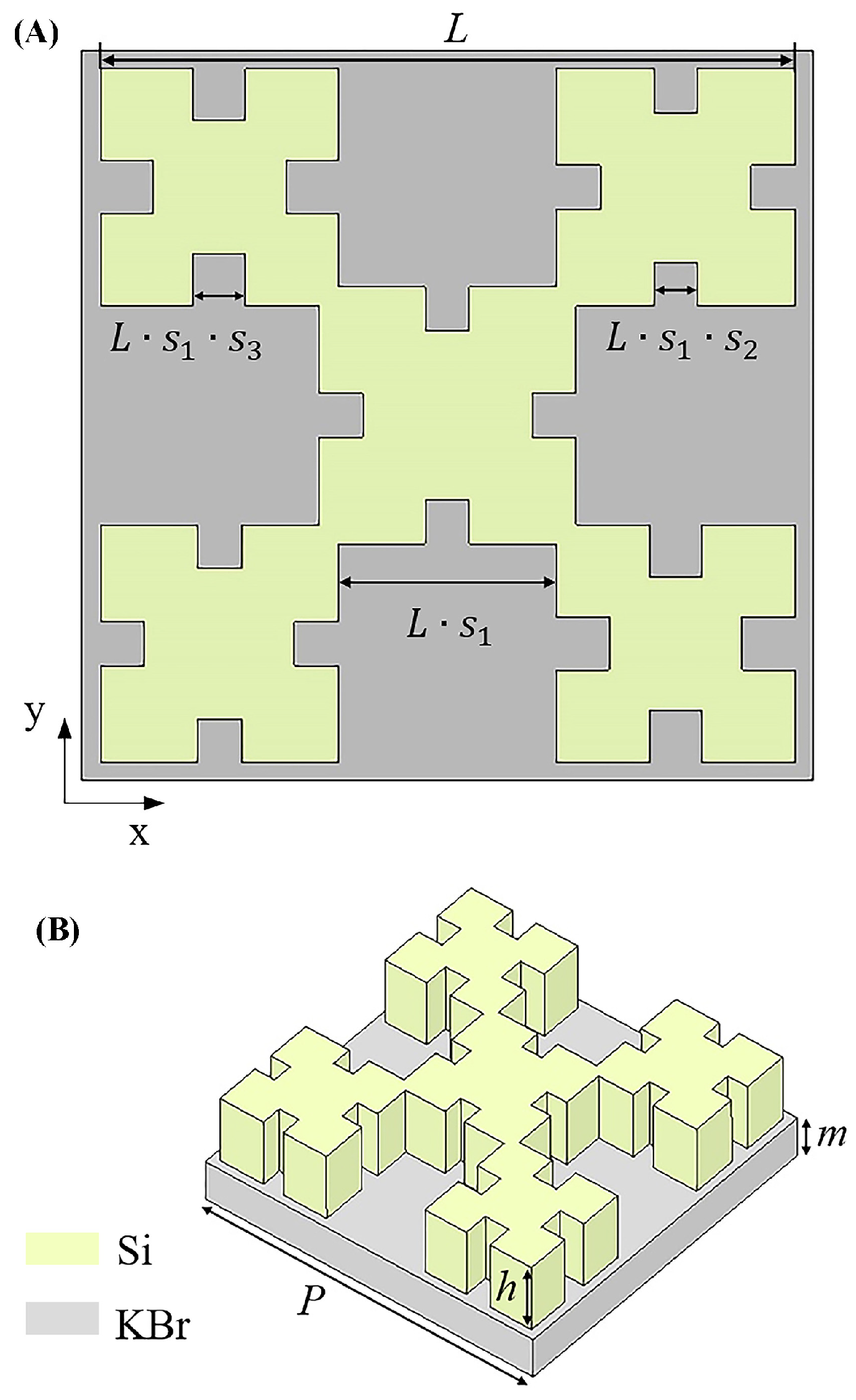
Figure 2.
The transmission spectra under various fractal factor difference .
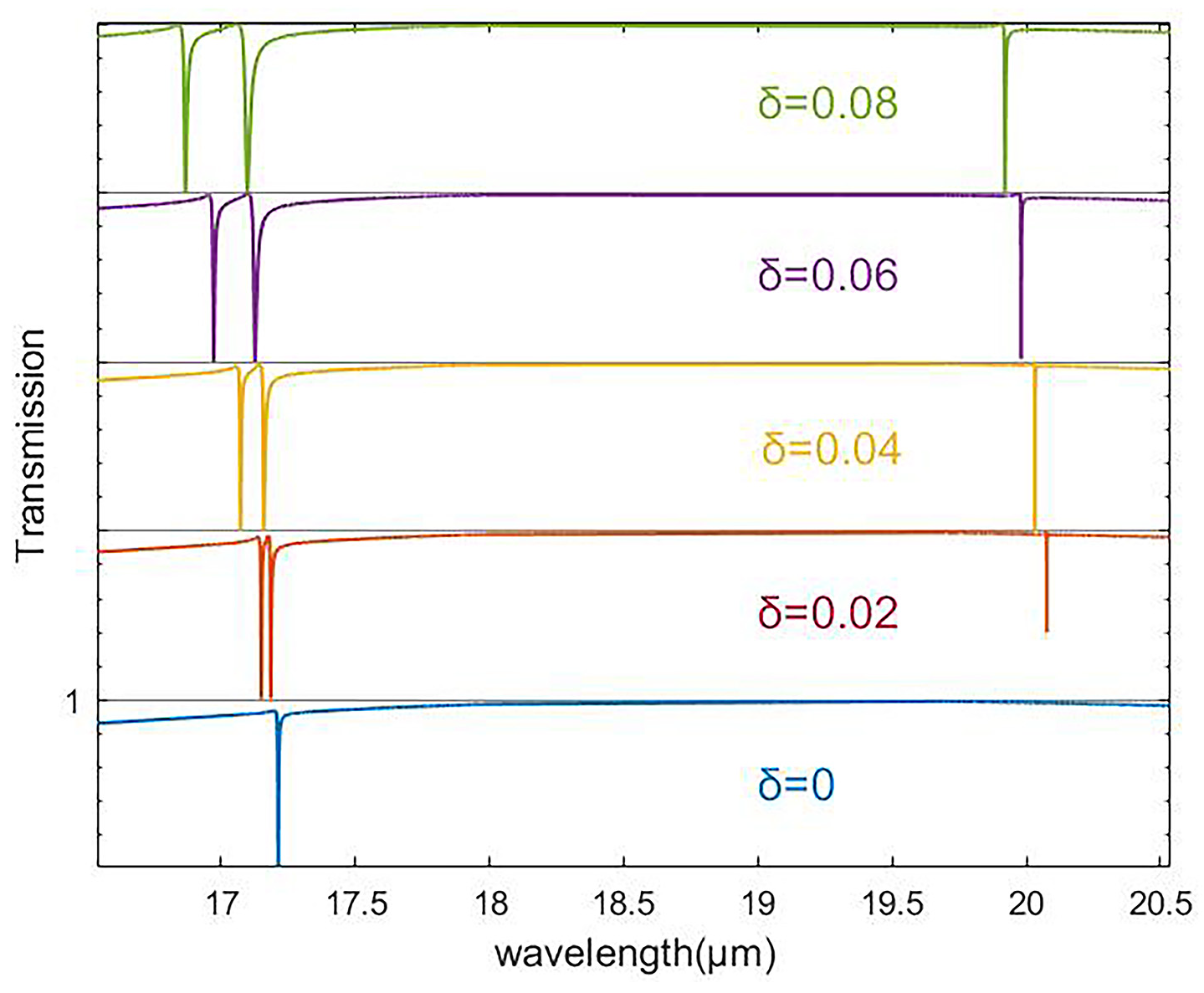
Figure 3.
Comparison of the Fano fitting and simulation results. (A), (B), and (C) are Fano fittings of mode1, mode2 and mode3 when . The solid curves are simulation results, and the dashed curves are Fano fitting results
Figure 3.
Comparison of the Fano fitting and simulation results. (A), (B), and (C) are Fano fittings of mode1, mode2 and mode3 when . The solid curves are simulation results, and the dashed curves are Fano fitting results
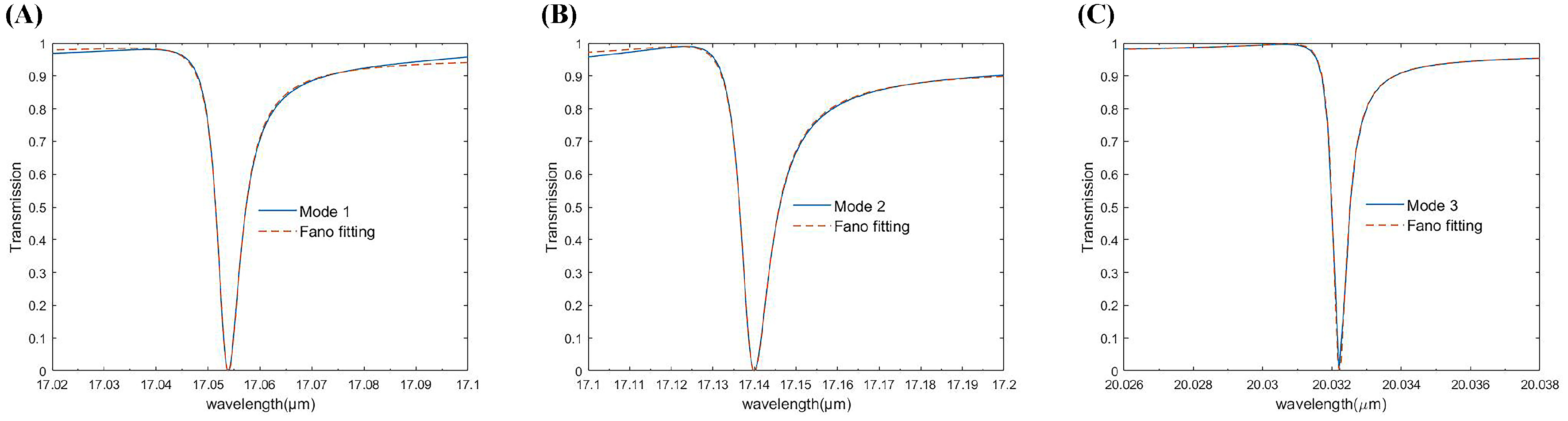
Figure 4.
The log-log plot of Q factors as a function of the asymmetric parameter of mode3. Solid black dots represent Q factors extracted from simulated spectra and the orange line shows the fitted inverse quadratic.
Figure 4.
The log-log plot of Q factors as a function of the asymmetric parameter of mode3. Solid black dots represent Q factors extracted from simulated spectra and the orange line shows the fitted inverse quadratic.
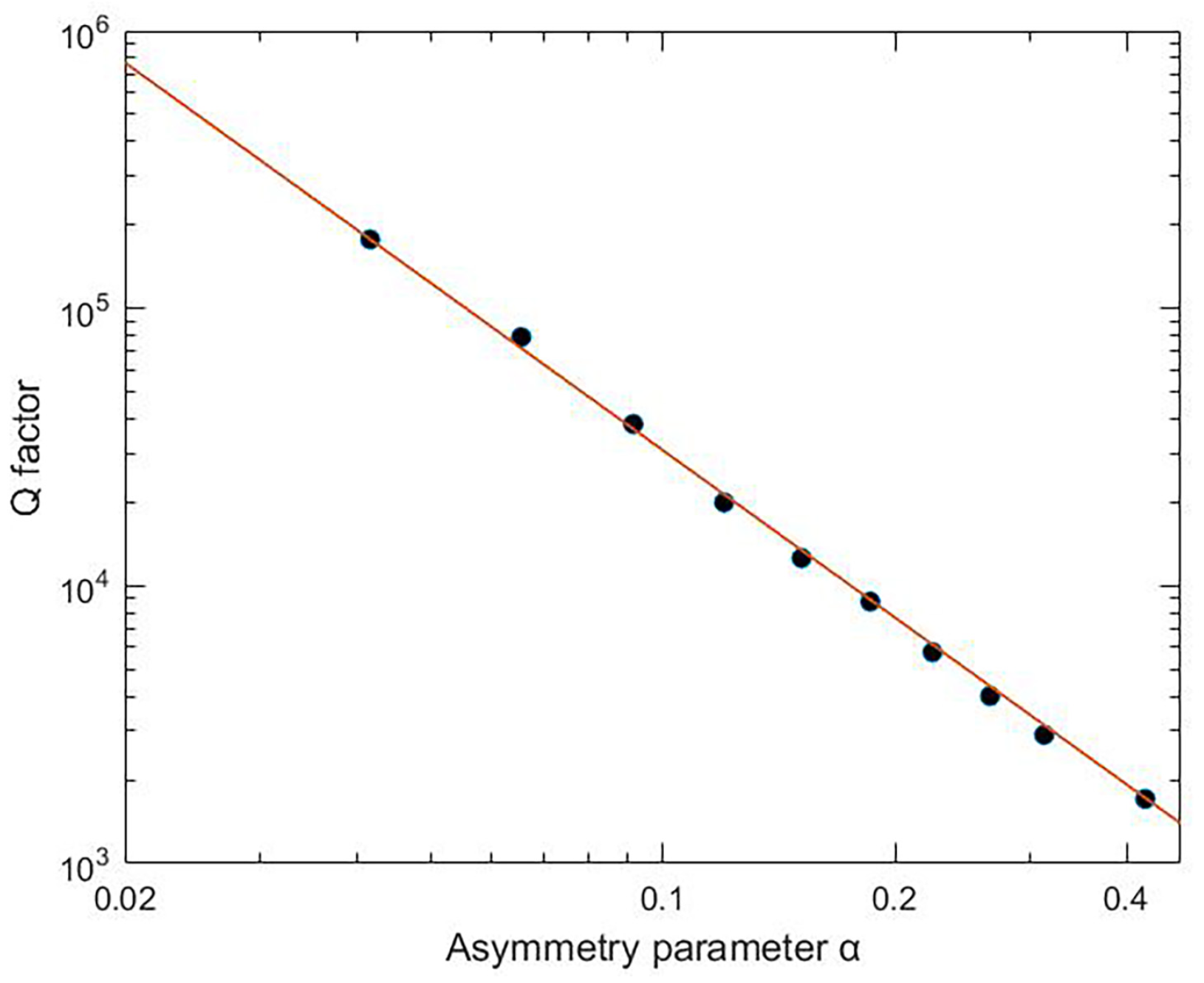
Figure 5.
Electromagnetic field distributions for different resonance modes. (A)-(H) cross-sectional patterns of electric field vector and enhancement in different plane for symmetric mode, mode 1, mode 2 and mode 3 respectively. (I)-(L) cross-sectional patterns of magnetic field vector and enhancement for above four modes. Cross-sectional patterns in x-y plane correspond to the height of highest electric field intensive with z-axis; those in x-z plane correspond to and those in y-z plane correspond to .
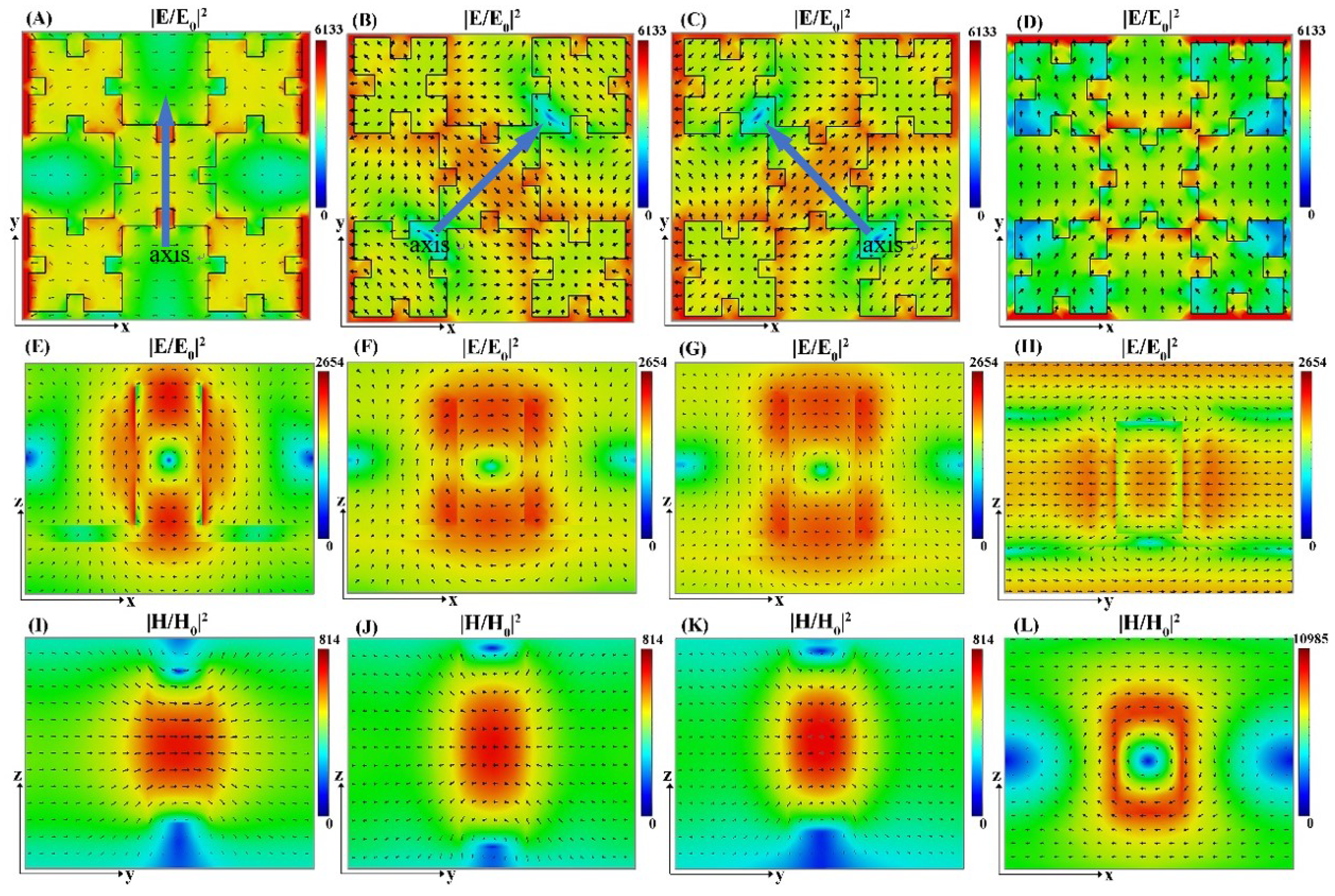
Figure 6.
The normalized scattered power by different multipole moments for (A)mode 3 and (B)mode1 and mode 2 (C)symmetric mode
Figure 6.
The normalized scattered power by different multipole moments for (A)mode 3 and (B)mode1 and mode 2 (C)symmetric mode
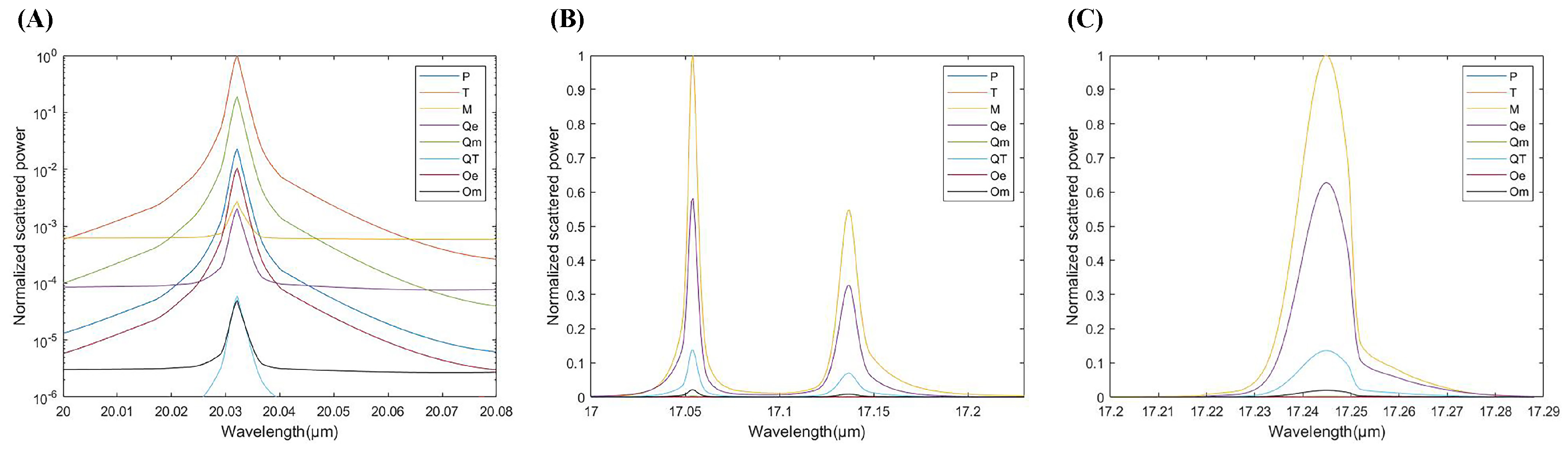
Figure 7.
Transmission spectra under x-polarization and y-polarization for(A)mode 3 (B)mode 1 and mode 2.
Figure 7.
Transmission spectra under x-polarization and y-polarization for(A)mode 3 (B)mode 1 and mode 2.
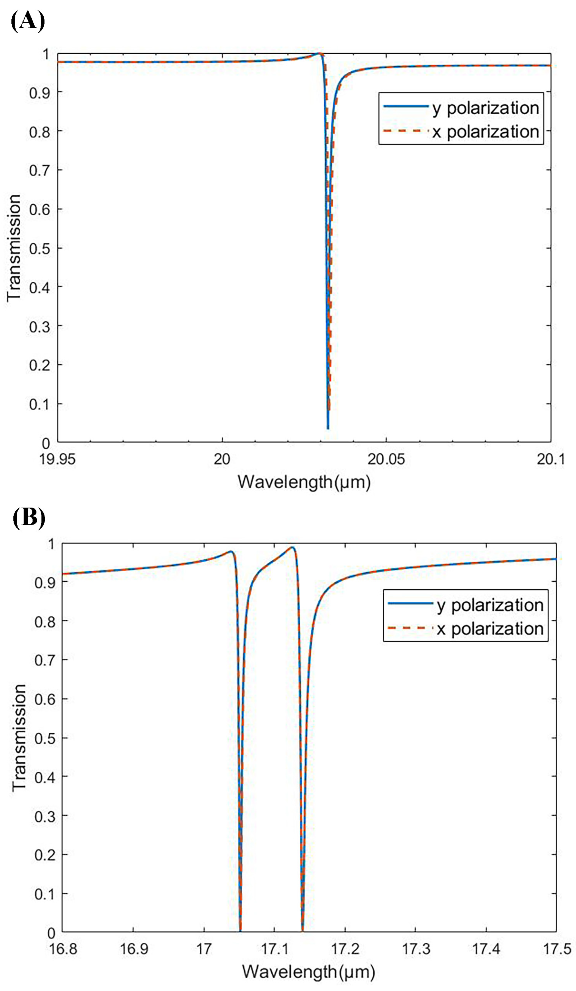
Figure 8.
Transmission spectra of the asymmetric metasurface structure with different(A) thickness of substrate m (B) height of nanodisk h and (C) period P
Figure 8.
Transmission spectra of the asymmetric metasurface structure with different(A) thickness of substrate m (B) height of nanodisk h and (C) period P
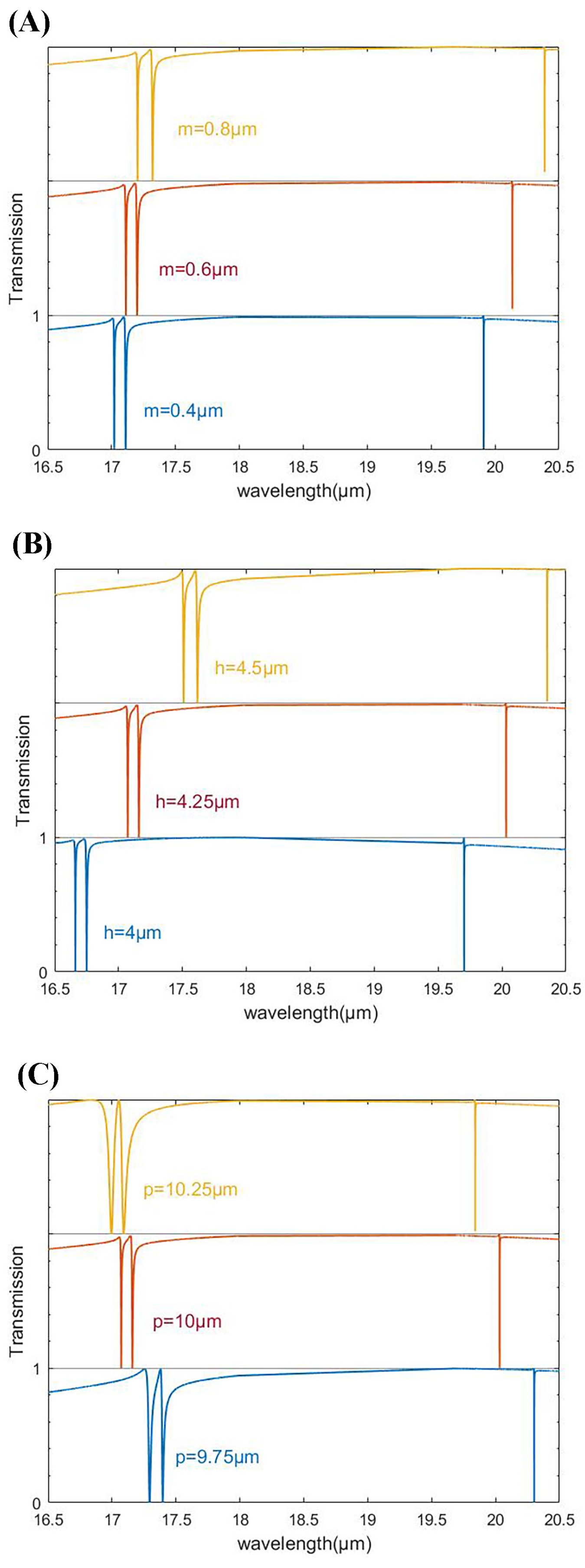
Figure 9.
Wavelength shift of mode3 versus height of water sample
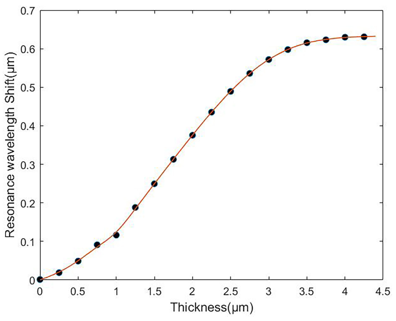
Figure 10.
Refractive sensing performance of metasurface sensor. Transmission spectra of (A)mode 3, (B)mode1 and mode 2 with different refractive indices. (C) Resonance wavelength shift of three modes with different refractive indices
Figure 10.
Refractive sensing performance of metasurface sensor. Transmission spectra of (A)mode 3, (B)mode1 and mode 2 with different refractive indices. (C) Resonance wavelength shift of three modes with different refractive indices
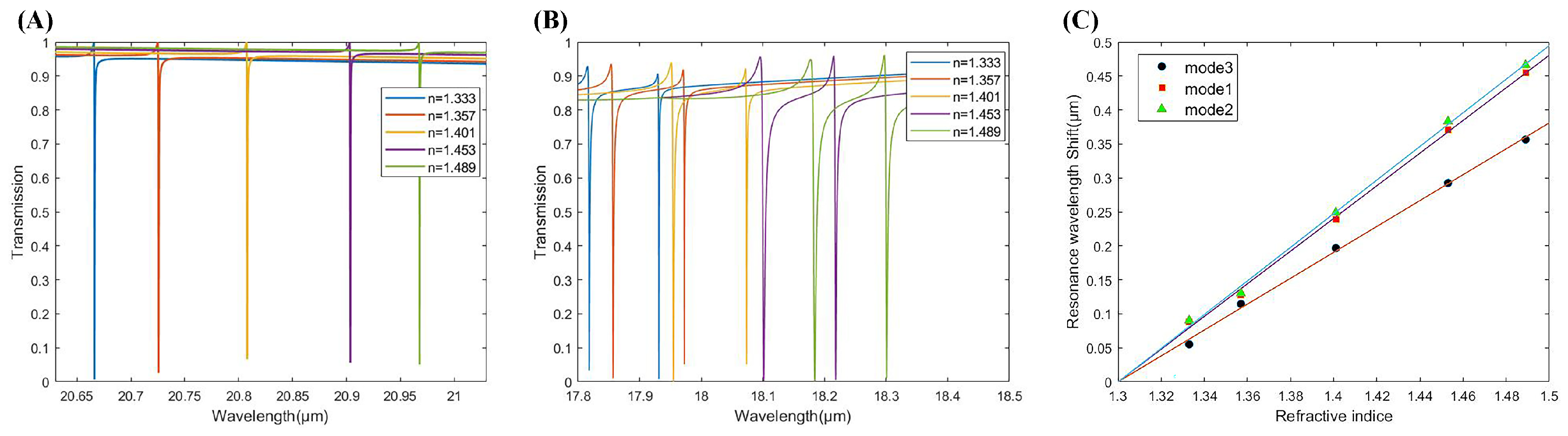

Table 1.
refractive index measurement performance of sensor proposed
| Mode | Sensitivity(m/RIU) | FOM |
|---|---|---|
| Mode1 | 2.404 | 724 |
| Mode2 | 2.475 | 1123 |
| Mode3 | 1.905 | 5625 |
Disclaimer/Publisher’s Note: The statements, opinions and data contained in all publications are solely those of the individual author(s) and contributor(s) and not of MDPI and/or the editor(s). MDPI and/or the editor(s) disclaim responsibility for any injury to people or property resulting from any ideas, methods, instructions or products referred to in the content. |
© 2025 by the authors. Licensee MDPI, Basel, Switzerland. This article is an open access article distributed under the terms and conditions of the Creative Commons Attribution (CC BY) license (http://creativecommons.org/licenses/by/4.0/).
Copyright: This open access article is published under a Creative Commons CC BY 4.0 license, which permit the free download, distribution, and reuse, provided that the author and preprint are cited in any reuse.


