Submitted:
10 April 2025
Posted:
10 April 2025
You are already at the latest version
Abstract
Macroalgae are an integral part of estuarine primary production, however their excessive growth may have severe negative impacts on the ecosystem. Although it is generally believed that algal blooms may be caused by a combination of excessive nutrients and temperature, their occurrences are hard to predict, and quantitative monitoring is a logistical challenge which requires development of reliable and inexpensive technique. This can be achieved by implementation of processing algorithms and indices on multi-spectral satellite images. Tuggerah Lakes estuary on the Central Coast of NSW was studied because of the regular occurrences of blooms, primarily of green filamentous algae. The detection of algal blooms based on the red-edge effect of the chlorophyll provided consistent results supported by direct observations. Floating Algae Index (FAI) was chosen as the most accurate index detecting algal blooms in shallow areas. Logistic regression was implemented where FAI was used as a predictor of two clusters, “bloom” and “non-bloom”. FAI was calculated for multi-spectral satellite images based on pixels of 20x20 meters, covering the entire area of the Tuggerah Lakes. Seven sample points (pixels) were chosen, and the optimal threshold was found for each pixel to assign it to one of the two clusters. Logistic regression model was trained for each pixel; then the optimal parameters for its coefficients and the optimal classification threshold were obtained by cross validation and bootstrapping. Probabilities for classifying clusters as either “bloom” or “non-bloom” were predicted with respect to the optimal threshold. The resulting model can be used to estimate probability of macroalgal blooms in coastal estuaries allowing quantitative monitoring through time and space.
Keywords:
algae bloom
; satellite photos
; GIS index
; logistic regression
1. Introduction
Macroalgae (multicellular seaweeds) are important contributors to estuarine primary production. They normally grow in estuaries throughout the year, but in warm seasons may significantly increase in biomass resulting in the so-called algal blooms. This is especially common in shallow estuaries throughout the world (Valiela et al. 1997) and can significantly impact the entire ecosystem by inducing hypoxia, smothering seagrasses, and ultimately leading to the loss of estuarine biodiversity (Lavery et al. 1991, Raffaelli 1998, Cummins et al. 2004, Lyons et al. 2012, Wang et al. 2012, Lewis and DeWitt 2017) Optimal temperature for the maximum growth of macroalgae is 25-30oC (Larcher 1980), which may be a reason why macroalgal blooms occur in the seasons when water temperature is within these limits. Low water exchange between an estuary and the sea promotes the accumulation of nutrients which support algal growth in wide areas of shallow warm water (Deng et al. 2018, Paulimer et al. 2018). Therefore, rapid increase in algal biomass of common opportunistic algae such as Ulva (formerly Enteromorpha) intestinalis, Chaetomorpha linum, and other surface-floating species may serve as an indicator of water eutrophication caused by urban runoff from extensive development of surrounding areas or treated wastewater (Cohen 2002). Algal blooms can be an indirect indicator of unsustainable agriculture, insufficient wastewater treatment, changes of hydrological processes due to extensive development of the land and human population growth, or any other disturbances of natural balance of estuaries. Tracking and recording the dynamics of algal growth by remote sensing can be used as an environmental monitoring tool which is suggested for different parts of the world (Alharbi, 2022; Medina-Lopez et al. 2023).
Despite the widespread nature of macroalgal blooms in estuaries throughout the world (Valiela et al. 1997; Lyons et al. 2012), there is very little data on their temporal and spatial dynamics. Monitoring algal blooms at different temporal and spatial scales is the first crucial step in trying to understand the factors that correlate with the presence of the blooms and, ultimately, in developing predictive capabilities for effective management and control of excessive algal growth.
One of the challenges of effective monitoring is developing reliable and non-expensive techniques of measuring algal biomass and/or the area of the blooms. Substantial efforts have been placed into development of measurement techniques that would allow effective monitoring of the blooms at large scales in multiple estuaries (Scanlan 2007; Zhang 2019). As direct measurements in the field are impractical, especially at very large scales, remote sensing is the most promising tool for quantifying and mapping distribution and abundance of floating macroalgae.
In ecological studies, the use of satellite images is an effective non-invasive method of observation allowing monitoring at large spatial scales. Analysis of multi-spectral data enables the detection of areas with certain reflection pattern, or spectral signature. Detection of algal blooms using spectral signatures of pigments was suggested after this approach has been successfully implemented for biomass measurements of terrestrial vegetation (Rouse et al. 1974; Richardson 1996). The detection of algal mass by remote sensing is literally the detection of light reflection patterns of individual pigments common for the algae (Buschmann et al. 2012, Lillesand et. al. 2015).
The biological role of photosynthetic pigments is absorbing light energy and then transferring it to photosynthetic reaction organelles or re-emitting excessive energy at longer wavelengths to prevent photodamage of the cell. The distinctive feature of all types of chlorophyll is fluorescence in near infra-red diapason, when the lowest reflectance in the range of 630-650 nm changes to the highest in near infra-red of 685±25nm (Morton 1975, Horler et al. 1983; Gower et al. 2004). This produces the so-called “red-edge” effect, which is used as a specific optical feature in chlorophyll detection (Miyashita et al. 1996, Croft and Chen 2017).
Analyses of satellite images based on the “red edge” effect have been widely used to estimate chlorophyll activity in terrestrial plants (Rouse et al. 1974; Buschmann et al. 2012) and for detecting algal blooms on large areas such as the Yellow Sea (Hu 2009; Keith 2009, Alawadi 2010, Xing and Hu 2016; Hu et al. 2017). Initially, only massive bloom events could be detected using images obtained from Moderate Resolution Imaging Spectroradiometers (MODIS) on board of Terra and Aqua satellites due to its 500m resolution (Shen et al. 2012). However, with recent enhancements of satellite sensors more detailed images could be obtained, which allowed monitoring smaller areas (Cao et. al. 2021). Several algorithms were developed to process raw satellite data to use them for remote sensing monitoring of terrestrial and aquatic vegetation. The results of these algorithms, or indices, serve as a base for machine learning techniques for algal blooms detection (Medina-Lopez et al. 2023). The index also can be used to quantify harvestable macroalgal biomass accumulations (Joniver et.al. 2019)
Mathematical models proved to be a reliable tool in the studies of species dynamics (such as phytoplankton, algae, and other water-dependent fauna) in connection with environmental conditions as water salinity or toxins release during harmful algae bloom (Sukhinov et al, 2021). Fractional regression model was implemented in the study of rural production performance (da silva e Souza et al. 2022). Modelling proved to be effective in reduction of harvest operations costs (Albornoz et al. 2022). In this study the result was obtained by the development of the model based on logistic regression algorithm and training it on the sample point data.
The primary aim of this study was to assess and identify the most reliable among known indices for the detection of macroalgal blooms. To allow the analysis to be used at different sun angles and light intensity, the index should be ratio-dependent (Lee, 1997). Therefore, six indices were selected for further comparison: NDVI (Normalized Difference Vegetation Index), SABI (Surface Algal Bloom Index), FAI (Floating Algae Index), ABDI (Algal Bloom Detection Index), MCI (Maximum Chlorophyll Index), VB-FAH (Virtual Baseline Floating macroAlgae Height).
The secondary aim was to develop effective techniques for identifying and quantifying macroalgal blooms, facilitating efficient monitoring and measurement of their abundances.
2. Methods
2.1. Selection of “Candidates” for the Optimal Index
For the selection of the best index for macroalgae bloom detection, Web of Science and Scopus databases were searched following the methodology of Lyons et al. (2012). The focus of search were algorithms for interpretation of remote sensing data for chlorophyll spectral signature detection.
The search terms for multi-spectral satellite images interpretation and keywords for chlorophyll activity were combined using Boolean operator “AND”. The keywords for chlorophyll reflectance and algal blooms were separated by the operator “OR” and then combined into a search string. The following search terms for remote sensing and multi-spectral data processing have been used:
“Satellite Remote Sensing” OR “Remote sensing” OR “Multi spectral” OR “Spectral Index” OR “Chlorophyll Index” OR “Spectral signature” OR “Chlorophyll fluorescence” OR “Vegetation monitoring” OR “Water leaving radiance” OR “Reflectance” OR “Red edge effect” OR “MODIS” OR “ERTS” OR “MERIS” OR “Sentinel” OR “Bloom monitoring”.
The following terms were used to search for algorithms and indices:
“NDVI” OR “Normalized Difference Vegetation Index” OR “FAI” OR “Floating Algae Index” OR “NDAI” OR “Normalized Difference Algae Index” OR “SAI” OR “Scaled Algae Index” OR “SABI” OR “Surface Algal Bloom Index” OR “FLH” OR “Fluorescence Line Height”
The following terms were used to search for information on macroalgal blooms:
“Macroalgae” OR “Macroalgal Blooms” OR “Floating vegetation” OR “Chlorophyll content” OR “Green macroalgae” OR “Floating macroalgae” OR “Ulva” OR “Enteromorpha” OR “Chaetomorpha”
As a result, information about existing indices which can be used for macroalgal blooms detection was collected, and six indices were implemented in raster analysis of the study area. The initial study of algal blooms and verification of data on the ground was done on the Tuggerah Lakes on the Central Coast, New South Wales, located 70 km north of Sydney. Tuggerah Lakes system consists of three interconnected lakes that form a saline barrier estuary of approximately 80 km2 area and an average depth of 2.4m. The estuary experiences regular macroalgal blooms (Batley et al. 1990, Scott 1999), which makes it optimal for satellite, drone, and on-ground observations.
For quantitative validation of our interpretation of the satellite data, the aerial photos were taken by the drone (DJI Phantom 4 Pro V2.0, camera DJI FC6310S) flying over the Chittaway bay area of Tuggerah Lake at the height of approximately 30 m. The images were georeferenced, the contours of algal bloom mats digitized, and the area measured using ESRI ArcGIS 10.7 software. Simultaneous capture of satellite images and drone photos involved using satellite images from the same date as the drone imagery. Bloom data obtained by index implementation on multi-spectral satellite images were compared with drone photos and the results of the direct observation to select the best performing index formula. Performance of the index was defined as the best correspondence with macroalgal mats contours, digitized from drone photos. The efficiency of each index was calculated as the ratio of the sum of true positives and true negatives to the total sum of pixels. It was applied to multi-spectral satellite data spanning from 2019 to 2023, involving the processing of a total of 170 images. Sample points were randomly selected at the places where blooms were observed on a regular basis.
2.2. Logistic Regression Model
Eleven training data sets were used, each of which had 166 records or timesteps collected over 4 years (dates 01/01/2019 to 18/02/2023). For all timesteps for each of the eleven data set points “bloom”/“non-bloom” status was established. This status was used along with the date when image was taken to train the model to detect the probability of the bloom using logistic regression. The timesteps for these records were irregular due to varying cloud cover, which completely obstructed aerial visibility on some days. As an algorithm of algae bloom detection, the single variable logistic regression was used. Analytically this model is given by the equation:
(1)
The variable x is an index value, and p(x) is an output which is interpreted as a probability of a bloom presence. For each pixel in the model the value of p(x) (1) has been estimated using the maximum likelihood method. Then the estimated values and were used for determining the probability .
The probability threshold was established based on index values for binary (“bloom”/“non-bloom”) classification, quantified as 0 and 1 respectively. For this estimation the Python language was utilized. After implementation of bootstrapping technique, the optimal threshold was found for each of the points. Cross-validation of the prediction function was made to classify “bloom” / “ non-bloom” events with respect to the optimal threshold. The cross-validation procedure is described in the special section below.
The algorithm is as follows: the given pixel classified as a “bloom” if the estimated value exceeded some threshold po, and non-blooming otherwise. Therefore, the blooming prediction algorithms were established for each pixel (sample point), using three parameters, , and po. Optimal thresholds po were identified by minimizing the classification error: percentage of wrongly classified pixel values.
Sample points on the lake were selected in areas where bloom occurrences were most frequent (Figure 1). Other features of those places which can affect the index results (seagrasses presence, shallow or turbid water) were also considered when selecting control points. Having those obstacles was important for selecting the most accurate threshold. For comparison, points where no bloom occurred were also chosen, but they were subsequently discarded during further processing as they were deemed unnecessary for training of the model.
For index implementation we used Sentinel 2 multi-spectral images taken in 2019-2023 years.
Results show overlap values attributed to “bloom” and “non-bloom” because of similarity of spectral characteristics of floating algae and seagrasses at the shallow water.
Therefore, we have an example of a binary classification, and the most logical approach to solve it is logistic regression (Figure 2).
During training and calibration of the model logistic coefficients which define the curve and probability threshold were calculated.
3. Results
3.1. Overview of Existing Indices
Satellite images are currently available as top-of-atmosphere radiances (level 1 data) and atmospherically corrected surface-leaving radiances (level 2 data) (Gordon and Wang, 1994). For calculations of any surface phenomena, like spectral signature of the algae, which is basically the light reflected from their surface, it is preferable to have level 2 data where the algorithms for atmospheric effects correction is implemented and unwanted effects are minimized (Gower et al. 2004, Matthews et al. 2012). Indices are transferable, which means that they can be implemented on rasters, obtained by different satellite sensors (MODIS, Landsat, Sentinel) (Li et al. 2017). All known indices are based on FLH (Fluorescence Line Height) algorithm which calculates the difference between reflection in 685±25nm (near infra-red, NIR) and in shorter (red) and in longer (infra-red) reflections. However, some of them introduced reflectance in green and blue bands to increase the capability of the algorithm to distinguish the spectral signature of the floating macroalgae from the surrounding water.
The first Index developed for terrestrial vegetation monitoring is TVI (Transformed Vegetation Index) It was made to be used with bands 5 and 7 of the satellite ERTS-1 (Earth Resources Technology Satellite-1) MSS (Multi-Spectral Scanner), or Landsat-1. The MSS recorded data in four spectral bands: green, red, and two infrared bands.
Where Band Ratio Parameter (BRP) is calculated as follows:
Where:
– reflection in near infra-red diapason , and
– reflection in red diapason (Rouse et al. 1974)
The difference between reflection in red and near infra-red diapasons proved to be a reliable basis for the development of future indices.
NDVI (Normalized Difference Vegetation Index) is calculated in the same manner as BRP. It is currently used for detection of chlorophyll concentration in terrestrial plants (Gitelson et al. 1999)
Where:
Xnir – reflection in near infra-red diapason , and
Xred – reflection in red diapason
Currently NDVI is a basic raster analysis tool for estimating the condition of terrestrial vegetation. However, it has limited use for aquatic flora because the sensor is unable to get reflectance in near infra-red diapason from submerged vegetation. Yet, NDVI works for the floating algal mats as spectral characteristics of macroalgae appearing above the water are similar to the terrestrial plants. It also gave a positive result for shallow waters near the shore indicating that index also picks up submerged seagrasses (see Figure 5).
FAI (Floating Algae Index) was developed for detection and mapping massive algal blooms on the sea surface. It shows chlorophyll activity and first was implemented on medium-resolution (250-500m) MODIS images. FAI detects the organisms with red edge effect of plant tissue above the water allowing separation of macroalgae from phytoplankton suspended in the water column (Hu, 2009). This index shows relative height of near infra-red peak relative to background value, which is interpolated from surrounding red and short-wave infrared (SWIR) wavelength values:
Where:
RRC(RED) is the Rayleigh-corrected top of atmosphere reflection in red diapason,
RRC(NIR) - Rayleigh-corrected top of atmosphere reflection in near infra-red diapason,
RRC(SWIR) - Rayleigh-corrected top of atmosphere reflection in short wave infra-red diapason,
λ(RED) – median wavelength in red diapason,
λ (NIR) – median wavelength in near infra-red diapason and
λ (SWIR) – median wavelength in short wave infra-red diapason.
Importantly, FAI is sensitive to water turbidity as it also reflects infra-red radiation and therefore can give false positive result (Wang et. al. 2011; Garcia et al, 2013). However, when used with Sentinel 2 images, it shows good precision when compared with detailed aerial photos (Figure 5).
NDAI (Normalized Difference Algae Index) uses the same scheme as NDVI that is based on difference between reflectance in red and NIR diapasons. This index works on atmospherically corrected data. The correction is based on the images taken in SWIR diapason.
Where - top of atmosphere reflectance in near infra-red diapason,
– atmospheric correction for near infra-red diapason,
- top of atmosphere reflectance in red diapason, and
– atmospheric correction for red diapason.
The index has large negative results for clean blue ocean waters which have low reflectance in both red and NIR diapasons. In turbid conditions, suspended inorganic particles in the water column cause higher reflectance in red and low in NIR. In this case, NDAI may show low positive or slightly negative values (i.e. indicating presence of algae when there are none). Algae have low reflectance in red and high in NIR, so the index will have high positive values when a macroalgal bloom is present (Shi and Wang, 2009).
SAI (Scaled Algae Index) is an algorithm used to calculate spatial extent of floating algae (Garcia et.al. 2013) Its implementation requires several steps. First, the index, which detects chlorophyll (NDVI or FAI), is calculated. Then odd-numbered square pixel region selected around each pixel, median value calculated for this region and applied to the central pixel. New raster is filled with these values. This resulting raster has the same configuration and number of pixels but a smoothed picture with high variability of an image removed.
Then the empirically selected threshold is applied, and all pixels are divided into “algae” and “non-algae” categories. This approach works well on large area of the Yellow Sea. However, the number of pixels on the side of square region which is used to extract median value needs to be smaller than the number of pixels across the entire area of the bloom, otherwise the high index values may be replaced with the lower median, and some data will be lost. For smaller lakes, the application of the median value can be skipped, and threshold can be applied directly on index raster. Resulting number of “bloom” pixels is used to calculate the area of the bloom. At the last step, the area of the bloom is calculated as a product of the number of pixels showing positive result (“bloom” pixel) multiplied by the area depicted by one pixel (spatial resolution of a sensor) This Index also considers the value of the “bloom” pixel and calculates relative algae coverage in the area covered by this pixel.
SABI (Surface Algal Bloom Index) is an empirical algorithm developed for processing MODIS images (Alawadi 2010). It is targeted to estimate the area of floating macroalgae. It uses the “red edge effect” in the nominator and incorporates blue and green bands in the denominator which supposed to make it less dependent to atmospheric effects and Rayleigh scattering. SABI is calculated as follows:
Where:
Xnir – reflection in NIR diapason ,
Xred – reflection in red diapason,
Xgreen – reflection in green diapason, and
Xblue – reflection in blue diapason.
SABI can be implemented on Sentinel 2 data and was considered in further analysis.
MERIS MCI (Medium Resolution Imaging Spectrometer - Maximum Chlorophyll Index) proved to be effective for detecting cyanobacteria blooms in turbid eutrophic waters where suspended matter increase reflection in visible diapason and can mask the chlorophyll spectral signature. It also detects surface blooms of microalgal films or floating macroalgae mats. However, for macroalgae its application is limited because of high chlorophyll content in their floating biomass, which may be compared to those in plants. In this case MCI may show “out-of-range” (too high) results as for terrestrial vegetation (Binding et al. 2013)
Based on MERIS data, MCI calculates the height of peak in reflection at 709nm against baseline formed by reflections at 681 and 753nm. But it is versatile and can be adopted for other satellite sensors bands with different wavelengths.
Where:
L – atmospherically corrected water-leaving reflection
681, 709 and 753 – central wavelengths of bands used in calculation.
VB-FAH (Virtual Baseline Floating macroAlgae Height) algorithm was developed for mapping macroalgal blooms in the Yellow Sea and proved to be insensitive to atmospheric effects and solar/viewing position (Xing and Hu, 2016). It is a peak-above-baseline method which uses the difference between artificial baseline and height of reflectance peak in NIR. The difference from the previously described MERIS MCI is that the baseline is formed by reflections in red and green diapasons, which, in the case of floating algal mats, has smaller values then reflectance in NIR:
As this index was developed to be used with Sentinel 2 images to pick up macroalgae mats it was selected for analysis too.
FGTI (Floating Green Tide Index) approach is based on the enhancement of raw digital data using a matrix of coefficients developed for each sensor. This increases the difference between the clear water and floating algal mats. This method allows the use of images without atmospheric correction and can detect macroalgae through a thin cloud coverage and has been successfully used for monitoring floating Ulva prolifera mats in the Yellow sea (Zhang et al. 2019). Because this approach does not include any map algebra to select bloom areas and appear to be sensor-dependent (coefficients are unique for each sensor), we did not use it further.
ABDI (Algal Bloom Detection Index) was developed for use with Sentinel 2 Bands (Cao et. al, 2021):
Where:
RRED - reflection in red diapason (645 – 665 nm),
RRE2 - reflection in red-edge 2 diapason (740nm),
RNIRn - reflection in near infra-red diapason (859-865 nm),
λRED – median wavelength in red diapason used (645 – 665 nm),
λRE2 – median wavelength in near infra-red diapason, and
λNIRn – median wavelength in narrow bear infra-red diapason.
ABDI takes advantage of extended red-edge bands as Sentinel 2 provides three diapasons for plant red-edge effect detection. It also uses green band where chlorophyll has the strongest reflection.
3.2. Selection of the Optimal Index
For floating macroalgae, having water surface as a background, initially seems to simplify the task. However, coastal shallow zones vary greatly in terms of vegetation composition and type, and not all of it can be attributed to macroalgal blooms. Seagrasses are also photosynthesize, but usually they do not constitute a problem unless found in very shallow water. For example, in the RGB image (Figure 3), only the top two fragments can be attributed to blooming, while the others should be classified as non-blooming, despite the visual similarity between fragments of the image taken on underwater seagrasses and the actual algal bloom. This was the challenge of classification—when spectral composition at certain points could be classified as both “bloom”/“non-bloom”. The outstanding spectral characteristic of the algal mat is high chlorophyll activity producing a red edge effect. Therefore, the challenge was to find the threshold index value, by which it will be possible to detect “bloom” pixels attributed to the algal bloom.
The following procedure was developed to select an index that best distinguishes coastal algal bloom occurring in shallow turbid water where seagrasses may also be present. A study area was chosen by the drone footage which was captured simultaneously with a satellite image. Six indices were applied to the same multi-spectral image fragment. Out of the six studied indices, two (NDVI and SABI) already had binary values, indicating pixels where bloom was detected or absent.
After calculating the values of the remaining four indices (FAI, VB-FAH, MCI, and ABDI) for each pixel in the selected fragment using ArcGIS Map Algebra, the results were reclassified using the Slice tool to standardize them for subsequent comparison. The Natural Breaks method was applied for greater contrast.
Following classification by the Slice method for all indices, a uniform threshold was established based on visual assessment, categorizing pixel values as either “bloom” or “non- bloom”. A threshold value of 100 was selected.
Therefore, six binary “bloom”/“non-bloom” rasters were obtained. The next step involved comparing these binary rasters with the results from the drone photo processing. Digitized contours of algal mats from the drone photo were overlaid onto the raster of the satellite image (Figure 3). Algal blooms could be easily identified from the drone images and, thus, pixels within detected algae mats were selected to determine true positive and negative, as well as false positive and negative pixels (Figure4).
Some difference in the total number of pixels for VB-FAH and MCI can be attributed to variations in the formulae for index calculation and the involved ranges.
To assess how accurately each index identifies true positive and negative values (i.e., “bloom”/“ non-bloom”), the following equation was used:
where:
IA is the index of accuracy (a larger value indicates better performance),
TP is the number of true positive pixels,
TN is the number of true negative pixels,
TPxls is the total number of pixels in the studied fragment of the satellite image with the index implemented.
As observed in Table 1, FAI demonstrated the highest efficiency and was therefore selected for further analysis and modelling.
3.3. Model Training and Cross-Validation
Seven pixels for which the information about blooming/non-blooming was recorded for 166 consequential days were selected as calibration data (Figure 1). However, the time periods between these days were not constant, because satellite photos were taken on the irregular time steps, for the reason of the meteorological conditions and characteristics of the satellite orbit. For each of these images, the grid-code, or FAI value was recorded. So, the calibration data was constituted from the seven data sets (for points 1 to 7, Figure 1), each of which had input (FAI value) and output (binary code 0 for non-blooming and 1 for blooming). For the model calibration, FAI values for each pixel were normalized:
z=,
Where x is an original FAI value at the sample point, x̄ is sampling mean and s is sampling standard deviation. Then logistic regression model was run on the normalized data along with naïve (basic) classification when positive values were attributed to bloom and negative to non-bloom.
Sensitivity of a model assesses the model's ability to identify all positive instances correctly. It calculates the proportion of true positives out of all instances that are algae bloom (true positives plus false negatives). Sensitivity provides insights into the model's ability to capture all occurrences of algae bloom. A high sensitivity value indicates a low number of false negatives.
To assess the practicability of the model its results were compared with the naïve classification. As can be seen from Table 2 and Table 3, logistic regression gives lower overall error rate.
Three model parameters – overall error rate, quantity of false negatives and false positives – were selected for the model training (calibration). As the values of these parameters could lead to the model overestimation, or artificial deflation of the calibration error, the cross-validation test has been implemented to select the model coefficients, which minimize the test error.
As a result of calibration, the logistic coefficients and were estimated for each of seven pixels (Table 4). The error minimization procedure was implemented for selecting the optimal value of the probability threshold po which corresponded to the maximum accuracy of the model. For each pixel threshold po was changed from 0.1 to 0.9 with a step of 0.1. Then the bootstrap resampling procedure was implemented 100 times for each value of the probability threshold. For each value of the threshold, the mean accuracy was calculated. Accuracy defined in this algorithm as a complement of the overall classification error: Acc=1-Err, where classification error Err was a percentage of wrongly classified values (sum of false positive and false negative divided to the total number of the observations).
Figure 6a,b demonstrate the error rate with respect to threshold values for the first of 100 bootstrap iterations implemented for the sample point 1 (Figure 6a) and sample point 7 (Figure 6b). One iteration was selected to make the graphical illustration clearer. On these figures blooming error mean percentage of bloom classified as non-bloom (percentage of false negative results) and non-blooming error is percentage of non-blooms classified as blooms (percentage of false positives).
To evaluate the effectiveness of the modelling approach, error rates were compared among the naïve forecast, optimal logistic regression, and bootstrap test. As shown in Table 2, Table 3, and Table 5, the overall error rates for the naïve forecast were consistently higher than those for the optimal logistic regression model and bootstrapping, with the latter two exhibiting similar performance. Figure 7 presents the total classification errors for all three models, where the solid line, representing the logistic regression model, remains consistently below the dashed line, which corresponds to the naïve forecast. The bootstrapping results (dotted line) closely align with those of logistic regression, exceeding them by no more than 0.02% at sample point 1 and no more than 0.1% at the remaining six sample points. These findings indicate that the model successfully passed the bootstrapping test.
4. Discussion and Conclusions
The current paper has two important components. First, it presents a new methodology for selecting an optimal index, which can be calculated by utilizing the information obtained from satellite photos and which can be then used for quantifying the algal blooms. The selected Floating Algae Index was used for binary classification of pixels constituting a waterway into blooming/non-blooming conditions. Second, a traditional logistic regression approach is used for indication the optimal threshold which allows to separate pixels into “bloom”/”non-bloom” categories.
The major contribution belongs to the first component. The methodology of selection of an optimal index for macroalgal bloom detection starts form selecting a short list of the candidate indices, which was done by the analysis of Web of Science and Scopus databases were searched following the methodology of Lyons et al. (2012). The focus of search were algorithms for interpretation of remote sensing data for chlorophyll spectral signature detection. The primary research question was which indices are compatible with Sentinel 2 multi-spectral data and may provide clear selection of floating macroalgae in the shallow or turbid water. After implementing this search 6 candidates were selected.
Then these six indices were compared to select the optimal one. These six indices were applied on the multi-spectral satellite image of Tuggerah lakes estuary where blooming is possible. Then the arbitrary selected threshold was used for classifying the pixels as “bloom” (the threshold is exceeded) and “non-bloom” (the threshold is not exceeded). The actual information about blooming is also available for these pixels, in the other words we are in the context of supervise learning. Therefore, the confusion matrix characteristics could be calculated.
The index of accuracy was used for comparing the selected six indices. This metric was calculated as a ratio of the sum of the true positive and true negative (numerator) and the total number of pixels in the studied fragment of the satellite image with the index implemented (denominator). Logically the largest value of the accuracy index indicates the better performance of the index. The FAI demonstrated the highest efficiency (0.711) and was therefore selected for further analysis and modelling. The proposed method is reliable and easy to use, and it can be implemented by GIS tools.
Next reported result was the implementation of the logistic regression model for selecting the optimal threshold for the FAI index, which could be used for determining the blooming in each pixel without detail analysis of the lake surface with the drones, but solely relying on the satellite information. The model was calibrated and validated for seven pixels in the Tuggerah lakes, where blooming has happened during the observation period. The optimal values for the regression coefficients and probability threshold were established using the bootstrapping method. As the value of FAI index is not available for the future this model cannot be used as it is for predicting algal blooms. However, it can be used for detecting the blooms for the sites of the waterways, where direct observation of blooming is not possible, but the satellite photos, which allow to determine FAI index, are available.
Thus, in the future the model based on macroalgae detection index can be effectively used for monitoring macroalgal blooms in estuarine coastal areas. It picks up the algal mats on the images very precisely if implemented on high quality satellite photographs. There are more possibilities of implementation of multi-spectral images for macroalgal blooms detection and for identification of the species of algae that may be potentially differentiated by more advanced sensors. With the advent of new and more advanced sensors, obtaining spectral signatures of different species of algae and availability of high-resolution multi-spectral images may provide opportunities for remote species identification.
The single variable logistic regression model (blooming against FAI index value) was developed for the seven sample pixels of the Tuggerah Lakes in order to establish reliable detection of algal blooms will allow quantitative monitoring of blooms through time and space. As the next step of this research, the model could be expended to the multivariable logistic regression by the inclusion of other variables, like season, water temperature or nutrients except the FAI index, as well as the previous period values of these variables (for example, by utilizing the dynamic regression approach), which could considerably increase its predictive power and, hence, our ability to take preventative management actions at the key periods of algal blooms.
Authors Contributions
All authors contributed to the study conception and design. Material preparation, data collection and analyses were performed by Mayya Podsosonnaya and Maria Schreider. Modelling was conceptualized and developed by Sergei Schreider. The first draft of the manuscript was written by Mayya Podsosonnaya, Maria Schreider and Sergei Schreider commented on previous versions of the manuscript. All authors read and approved the final manuscript.
Funding
Not applicable. The authors certify that they have no affiliations with or involvement in any organization or entity with any financial interest or non-financial interest in the subject matter or materials discussed in this manuscript.
Data Availability Statement
All data generated or analysed during this study are included in this published article. Sentinel 2 images are available at Copernicus Data Space Ecosystem portal https://dataspace.copernicus.eu/.
Acknowledgments
Authors express their gratitude to Dr Vincent Raoult (University of Newcastle) for his help with obtaining the drone images, to Mr Olivier Rey-Lescure (formerly of the University of Newcastle) for his assistance with the use of georeferencing of the images, and to Ms Gabrielle Potts-Todd (University of Newcastle) for digitising drone images. The Python and R codes for the logistic regression were written by Shubham Sharma, Rutgers Business School.
Conflicts of Interest
The authors declare no conflict of interest.
Abbreviations
(ABDI) Algal Bloom Detection Index
(BRP) Band Ratio Parameter
(FAI) Floating Algae Index
(FGTI) Floating Green Tide Index
(FLH) Fluorescence Line Height
(MCI) Maximum Chlorophyll Index
(MERIS) Medium Resolution Imaging Spectrometer
(MODIS) Moderate Resolution Imaging Spectroradiometer
(MSS) Multi-spectral Scanner
(NDAI) Normalized Difference Algae Index
(NDVI) Normalized Difference Vegetation Index
(NIR) Near Infra-Red
(SABI) Surface Algal Bloom Index
(SAI) Scaled Algae Index
(SWIR) Shorth Wave Infra-Red
(TVI) Transformed Vegetation Index
(VB-FAH) Virtual Baseline Floating macroAlgae Height
References
- Alawadi F (2010) Detection of surface algal blooms using the newly developed algorithm surface algal bloom index (SABI) Proc. SPIE 7825, Remote Sensing of the Ocean, Sea Ice, and Large Water Regions, 782506.
- Albornoz, V.M., Araneda, L.C. & Ortega, R. (2022) Planning and scheduling of selective harvest with management zones delineation. Ann Oper Res 316, 873–890.
- Alharbi B (2022) Remote sensing techniques for monitoring algal blooms in the area between Jeddah and Rabigh on the Red Sea Coast. Remote Sensing Applications, Society and Environment 30, 100935.
- Batley GE, Body DN, Cook BG, Dibb L, Fleming PM, Skyring GW, Boon PI, Mitchell DS, Sinclair RL (1990) The ecology of the Tuggerah Lakes System: a review: with special reference to the impact of the Munmorah Power Station. Stage 1: hydrology, aquatic macrophytes, heavy metals, nutrient dynamics. Report prepared for the Electricity Commission of New South Wales, Wyong Shire Council and the State Pollution Control Commission [consultancy report].
- Binding CE, Greenberg TA, Bukata RP (2013) The MERIS Maximum Chlorophyll Index; its merits and limitations for inland water algal bloom monitoring. J Great Lakes Res 39, 100-107.
- Buschmann C, Lenk S, Lichtenthaler HK (2012) Reflectance spectra and images of green leaves with different tissue structure and chlorophyll content. Isr J Plant Sci 60:1-2, 49-64.
- Cao M, Qing S, Jin E, Hao Y, Zhao W (2021) A spectral index for the detection of algal blooms using Sentinel-2 Multispectral Instrument (MSI) imagery: a case study of Hulun Lake, China, Int J Remote Sens 42:12, 4514-4535.
- Cohen R (2002) The effects of runoff on the physiology of Enteromorpha intestinalis: implications for use as a bioindicator of freshwater and nutrient influx to estuarine and coastal areas. UC Office of the President: UC Marine Council.
- Croft H, Chen JM (2017) Leaf Pigment Content. Reference Module in Earth Systems and Environmental Sciences. University of Toronto, Toronto, ON, Canada.
- Cummins SP, Roberts DE, Zimmerman KD (2004) Effects of the green macroalga Enteromorpha intestinalis on microbenthic and seagrass assemblages in shallow coastal estuary. Mar Ecol Progr Ser Vol.266: 77-87.
- Da Silva e Souza G, Gomes EG, and de Andrade Alves ER. (2022) Two-part fractional regression model with conditional FDH responses: an application to Brazilian agriculture. Ann Oper Res 314, 393–409.
- Deng X, Liu T, Liu CY, Liang SK, Hu YB, Jin YM, Wang XC (2018) “Effects of Ulva prolifera blooms on the carbonate system in the coastal waters of Qingdao”. Mar Ecol Prog Ser 605:73-86.
- Garcia RA, Fearns P, Keesing JK, Liu D (2013) Quantification of floating macroalgae blooms using the scaled algae index. JGR Oceans, Vol. 118, Issue 1, 26-42.
- Gitelson AA, Buschmann C, Lichtenthaler HK (1999) The Chlorophyll Fluorescence Ratio F735/F700 as an Accurate Measure of the Chlorophyll Content in Plants. Remote Sens Environ Vol. 69, Issue 3, 296-302.
- Gordon HR, Wang M (1994) Retrieval of water-leaving radiance and aerosol optical thickness over the oceans with SeaWiFS: A preliminary algorithm. Appl Optics 33: 443-452.
- Gower JFR, Brown L, Borstad GA (2004) Observation of chlorophyll fluorescence in west coast waters of Canada using the MODIS satellite sensor. Can J Remote Vol. 30, No. 1, 17-25.
- Horler DNH, Dockray M, Barber J (1983) The red edge of plant leaf reflectance. Int J Remote Sens 4:2, 273-288.
- Hu C, (2009) A novel ocean colour index to detect floating algae in the global oceans. Remote Sens Environ 113, 2118–2129.
- Hu, L. Hu C. Ming-Xia HE (2017) Remote estimation of biomass of Ulva prolifera macroalgae in the Yellow Sea. Remote Sens Environ Vol. 192, 217-227.
- Joniver C, Moore P, Woolmer A, Adams J (2019) Is sustainable harvesting of opportunistic macroalgae blooms an ecological, social and economic solution? International Seaweed Symposium, 10.13140/RG.2.2.30406.11849.
- Keith DJ (2009) Estimating Chlorophyll Conditions in Southern New England Coastal Waters from Hyperspectral Aircraft Remote Sensing. Remote sensing of Coastal Environments, ed. Weng Q, Indiana State University, 151-172.
- Larcher W (1980) Physiological Plant Ecology. 2nd ed. Springler: Berlin.
- Lavery PS, Lukatelich RJ, McComb AJ (1991) Changes in the Biomass and Species Composition of Macroalgae in Eutrophic Estuary. Estuar Coast Shelf Sci 33, 1-22.
- Lee Z, Carder KL, Steward RG, Peacock TG, Davis CO, Mueller JL Remote sensing reflectance and inherent optical properties of oceanic waters derived from above-water measurements, in Ocean Optics XIII 2963, S. G. Ackleson and R. J. Frouin, Eds., 160-166 (1997).
- Lewis NS, DeWitt TH (2017) Effect of Green Macroalgal Blooms on the Behaviour, Growth, and Survival of Cockles (Clinocardium nuttallii) in Pacific NW Estuaries. Mar Ecol Progr Ser. 582: 105-120.
- Li S, Ganguly S, Dungan JL, Wang WL, Nemani RR (2017) Sentinel-2 MSI Radiometric Characterization and Cross-Calibration with Landsat-8 OLI. Advances in Remote Sensing 6, 147-159.
- Lillesand TM, Kiefer RW, Chipman JW (2015) Remote Sensing and Image Interpretation. 7th ed. Wiley, USA.
- Lyons DA, Mant RC, Bullen F, Kotta J, Rilov G, Crowe TP (2012) What are the effects of macroalgal blooms on the structure and functioning of marine ecosystems? A systematic review protocol. Environ Evid 1:7.
- Matthews MW, Bernard S, Lain LR (2012) An algorithm for detecting trophic status (chlorophyll-a), cyanobacterial-dominance, surface scums and floating vegetation in inland and coastal waters', Remote Sens Environ 124, 637-652.
- Medina-Lopez E, Navarro G, Santos-Echeandia J, Bernardes P, Caballero I (2023) Machine Learning for Detection of Macroalgal Blooms in the Mar Menor Coastal Lagoon Using Sentinel-2. Remote Sens 15, 1208.
- Miyashita H, Ikemoto H, Kurano N, Adachi K, Chihara M, Miyachi S (1996) Chlorophyll d as a major pigment. Nature 383, 402.
- Morton AM (1975) Biochemical Spectroscopy. Vol. 1. New York: Wiley and Sons.
- Paulimer A, Tatlian T, Reveillac E, Le Luherne E, Ballu S, Lepage M, Le Pape O (2018) Impacts of green tides on estuarine fish assemblages. Estuar Coast Shelf Sci 213: 176-184.
- Raffaelli DG, Raven JA, Poole LJ (1998) Ecological Impact of Green Macroalgal Blooms. Oceanography and Marine Biology: An Annual Review 36, 97-125.
- Richardson LL (1996) Remote sensing of algal bloom dynamics, Bioscience, 46, 492-501.
- Rouse Jr JW, Haas RH, Schell JA, Deering DW (1974) Monitoring vegetation systems in the Great Plains with ERTS. In: NASA. Goddard Space Flight Center 3d ERTS-1 Symposium, Vol. 1/A, 309–317.
- Scanlan CM, Foden J, Wells E, Best MA (2007) The monitoring of opportunistic macroalgal blooms for the water framework directive. Mar Pollut Bull 55, 162-171.
- Scott A (1999) Ecological History of the Tuggerah Lakes. CSIRO Land and Water, Canberra.
- Shen L, Xu H, Guo X (2012) Satellite remote sensing of harmful algal blooms (HABS) and a potential synthesized framework. Sensors, 12 (6), 7778-7803.
- Shi W, Wang M (2009) Green macroalgae blooms in the Yellow Sea during the spring and summer of 2008. J Geophys Res 114, p. C120010.
- Sukhinov A, Belova Y, Chistyakov A, Beskopylny A, Meskhi B. Mathematical Modeling of the Phytoplankton Populations Geographic Dynamics for Possible Scenarios of Changes in the Azov Sea Hydrological Regime. Mathematics 2021, 9, 3025.
- Valiela I, McClelland J, Hauxwell J, Behr PJ, Hersh D, Fereman K (1997) Macroalgal blooms in shallow estuaries Controls and ecophysiological and ecosystem consequences. Limnol Oceanogr 42/5, p. 2, 1105-1118.
- Wang C, Yu R, Zhou MJ (2012) Effects of the decomposing green macroalga Ulva (Enteromorpha) prolifera on the growth of four red-tide species. Harmful Algae, 16. 12–19.
- Wang XH, Qiao F, Lu J, Gong F (2011) The turbidity maxima of the northern Jiangsu shoal-water in the Yellow Sea, China, Estuar Coast Shelf Sci 93, 202- 211.
- Xing Q, Hu C (2016) Mapping macroalgal blooms in the Yellow Sea and East China Sea using HJ-1 and Landsat data: Application of a virtual baseline reflectance height technique. Remote Sens Environ 178, 113–126.
- Zhang H, Qiu Z, Devred E, Sun D, Wang S, Yu Y (2019) A simple and effective method for monitoring floating green macroalgae blooms: a case study in the Yellow Sea. Optics Express, Vol. 27, No. 4, 4528 – 4548.
Figure 1.
Sample points for algorithm training selected in the study area.

Figure 2.
Bloom and non-bloom values distribution for control point 1 and probability threshold (po) estimation (see equation (1)).
Figure 2.
Bloom and non-bloom values distribution for control point 1 and probability threshold (po) estimation (see equation (1)).
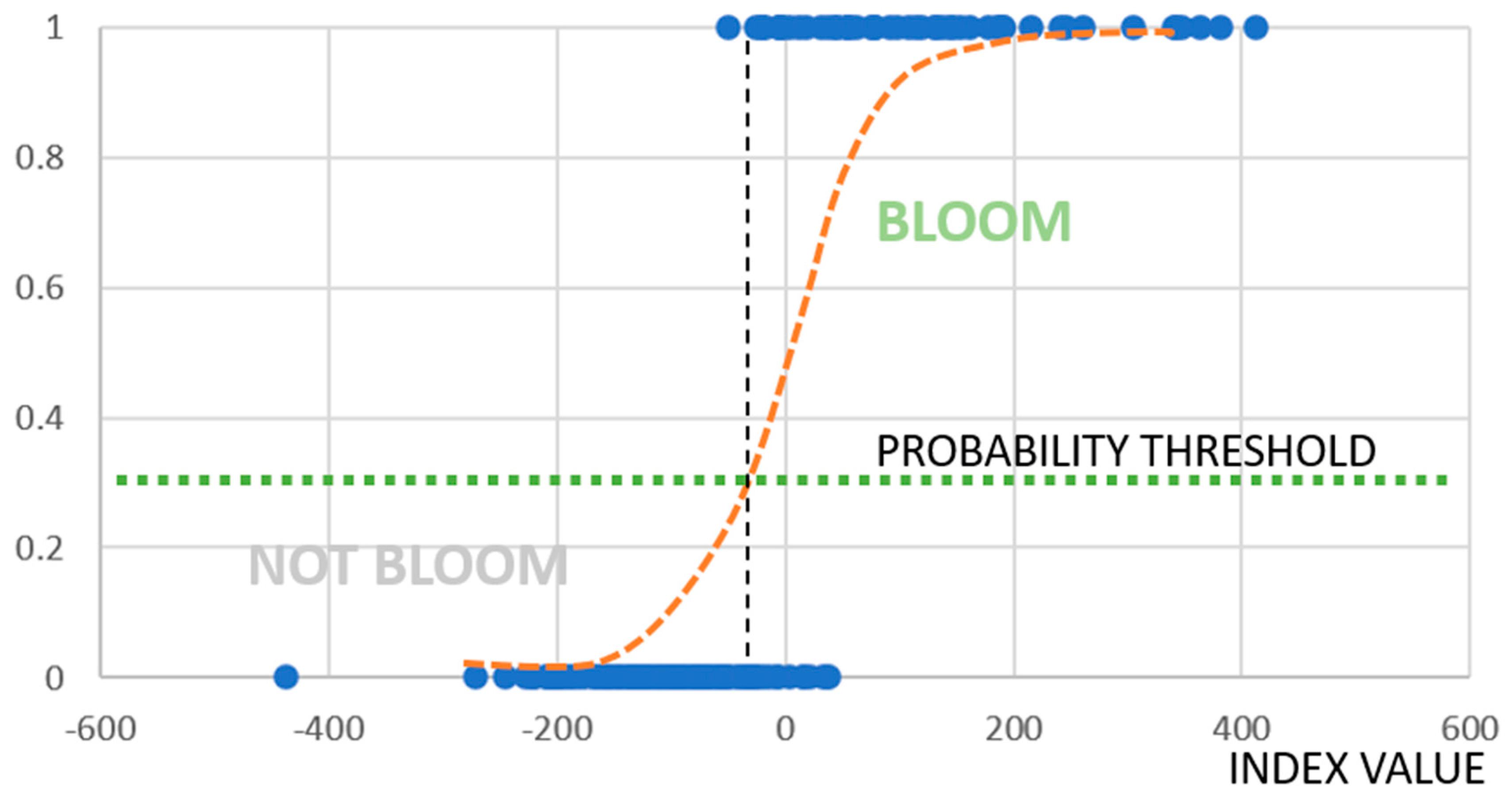
Figure 3.
RGB image of study area showing similarities in bloom and non-bloom areas.
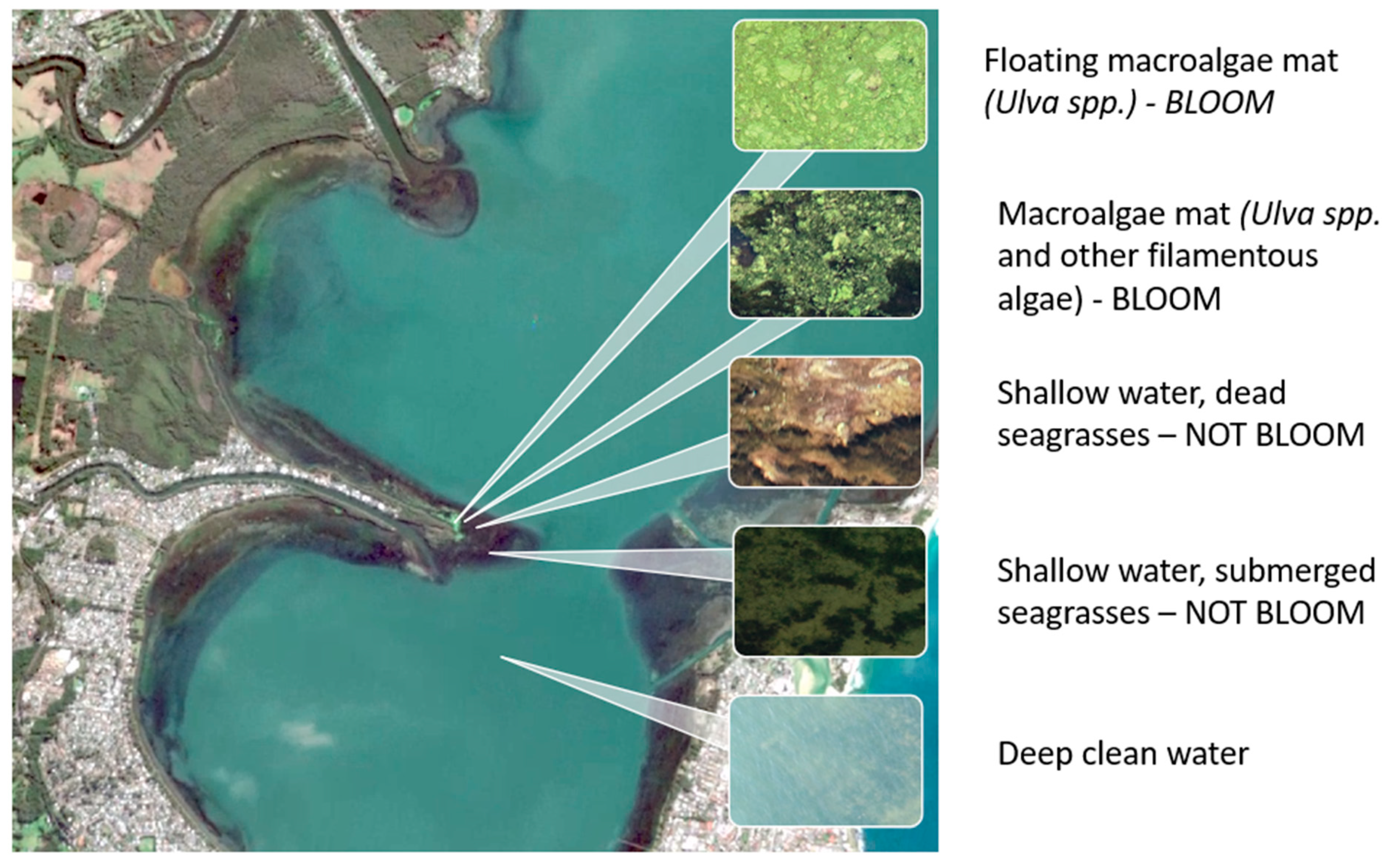
Figure 4.
Digitized algae mats obtained by the drone photo over the satellite image pixels.
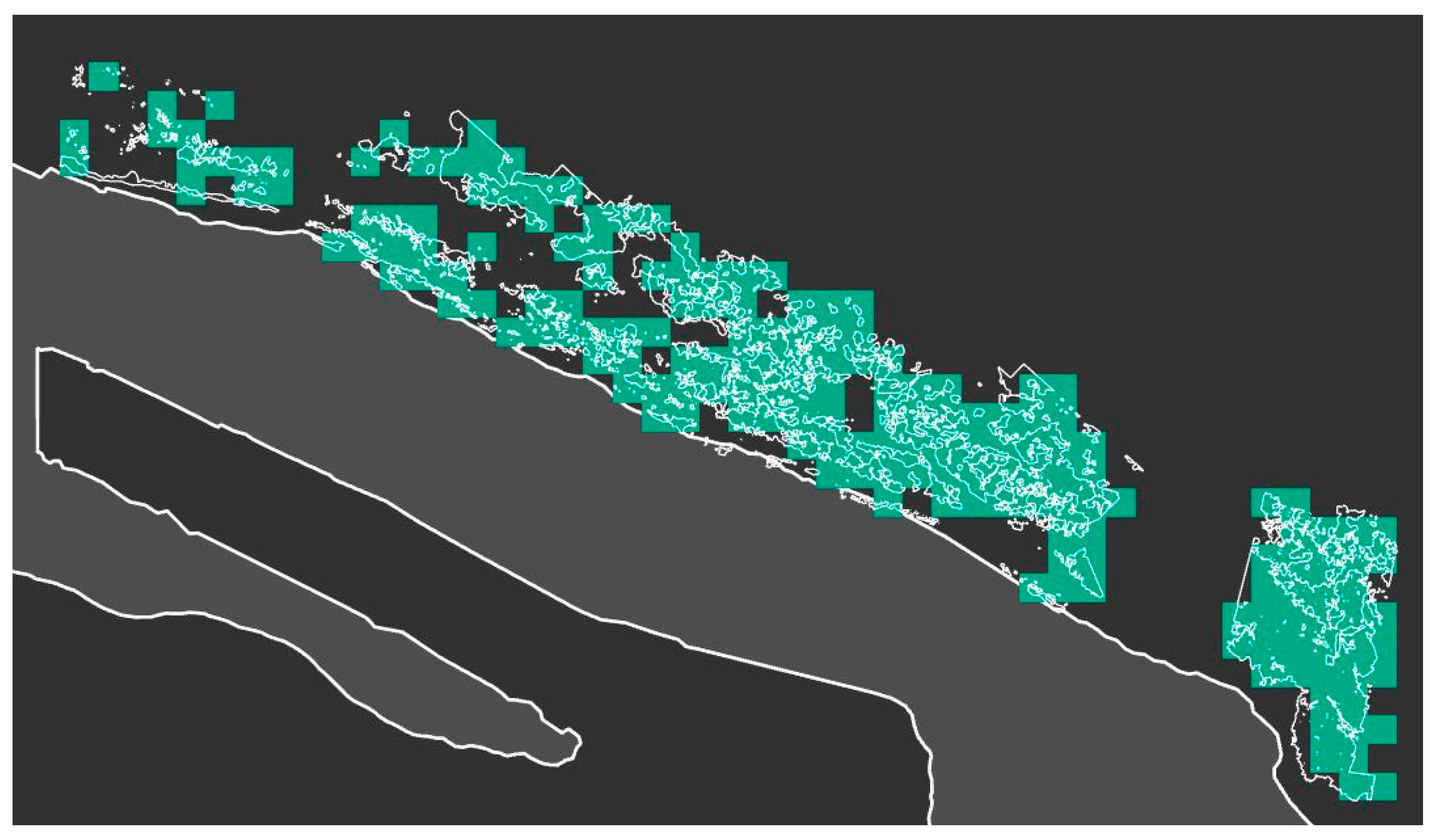
Figure 5.
Indices performance comparison.
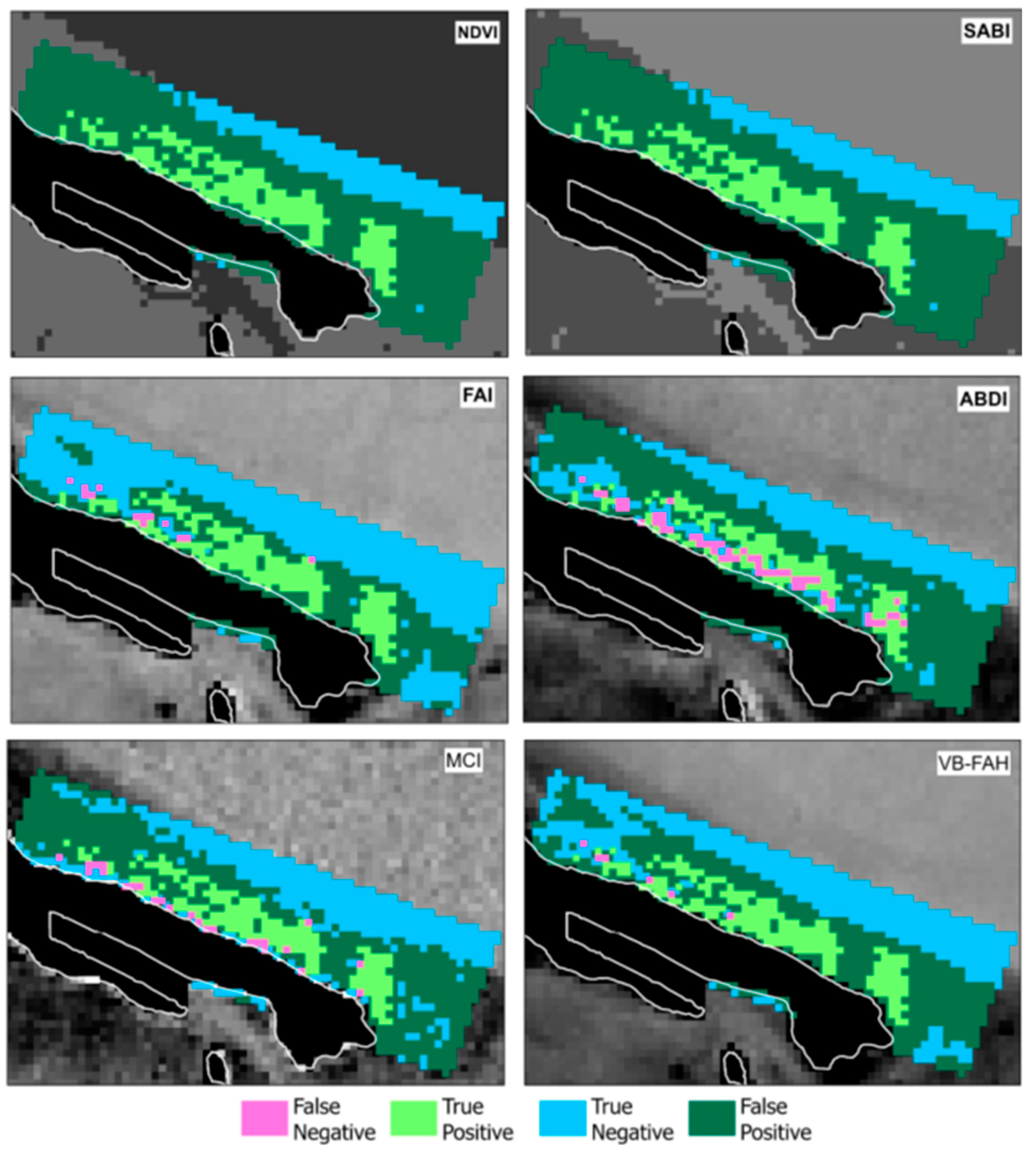
Figure 6.
a. Error rate as a function of threshold for sample point 1, for 100 bootstrap iterations. b. Error rate as a function of threshold for sample point 4, for 100 bootstrap iterations.
Figure 6.
a. Error rate as a function of threshold for sample point 1, for 100 bootstrap iterations. b. Error rate as a function of threshold for sample point 4, for 100 bootstrap iterations.
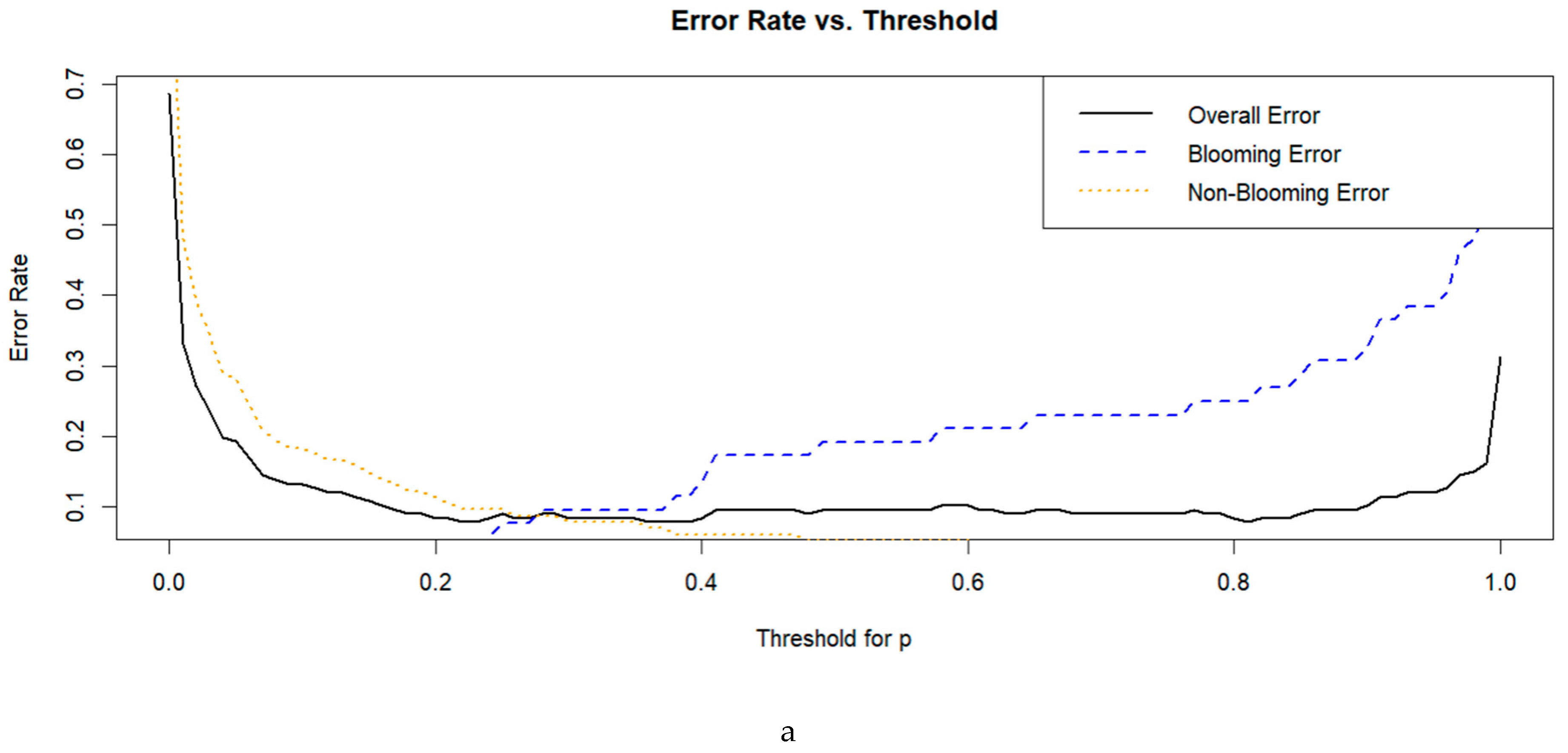
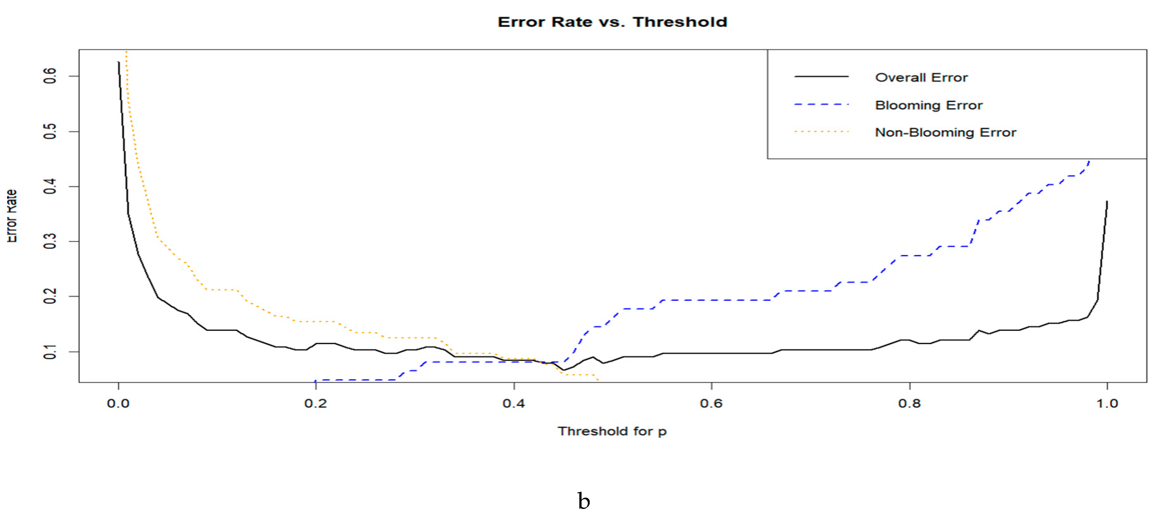
Figure 7.
Error rate for different classification at sample points 1 to 7.
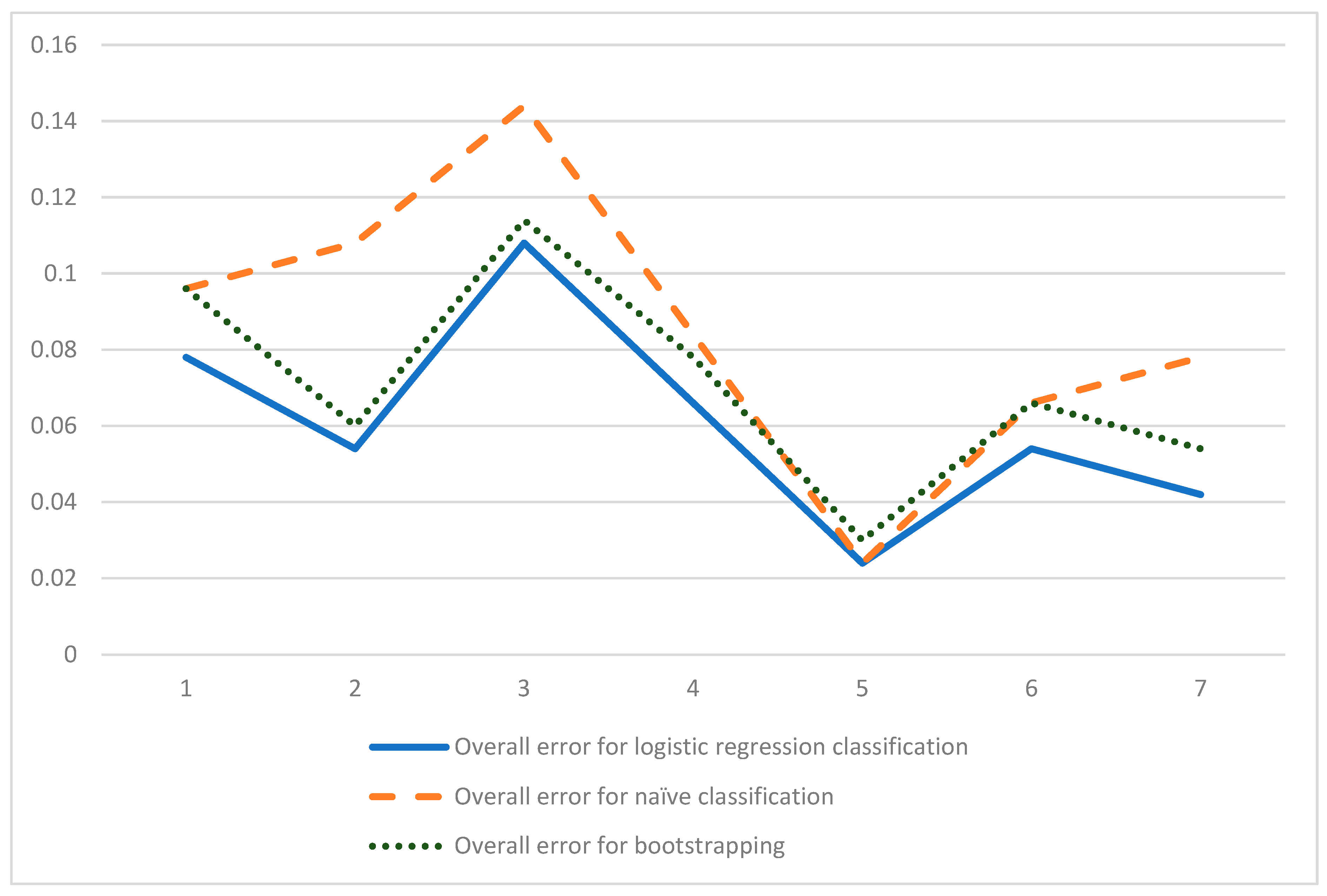

Table 1.
Pixel count for Indices performance analysis.
| Index | FAI | VB-FAH | MCI | ABDI | NDVI | SABI |
| True Positive | 170 | 172 | 157 | 130 | 183 | 183 |
| True Negative | 525 | 399 | 330 | 300 | 194 | 194 |
| False Positive | 270 | 372 | 442 | 495 | 601 | 601 |
| False Negative | 13 | 6 | 25 | 53 | 0 | 0 |
| Accuracy | 0.711 | 0.602 | 0.510 | 0.440 | 0.385 | 0.385 |
Table 2.
Confusion matrix for naïve classification.
| . | 1 | 2 | 3 | 4 | 5 | 6 | 7 |
| TP | 43 | 49 | 52 | 52 | 9 | 18 | 37 |
| FP | 9 | 3 | 7 | 10 | 1 | 3 | 2 |
| TN | 107 | 99 | 90 | 100 | 153 | 137 | 116 |
| FN | 7 | 15 | 17 | 4 | 3 | 8 | 11 |
| Overall Classification Error: (FP+FN)/(FP+TP+FN+TN) | 0.0963855 | 0.1084337 | 0.1445783 | 0.0843373 | 0.0240963 | 0.066265 | 0.0783132 |
| Sensitivity | 0.9386 | 0.8684 | 0.8411 | 0.9615 | 0.9808 | 0.9448 | 0.9134 |
Table 3.
Confusion matrix for the optimal basic logistic regression.
| 1 | 2 | 3 | 4 | 5 | 6 | 7 | |
| TP | 50 | 44 | 47 | 57 | 9 | 13 | 34 |
| FP | 2 | 8 | 12 | 5 | 1 | 8 | 5 |
| TN | 103 | 113 | 101 | 98 | 153 | 144 | 125 |
| FN | 11 | 1 | 6 | 6 | 3 | 1 | 2 |
| Overall Classification Error: (FP+FN)/(FP+TP+FN+TN) | 0.0783132 | 0.0542169 | 0.108433 | 0.066265 | 0.0240963 | 0.0542169 | 0.0421686 |
| Sensitivity | 0.9035 | 0.9912 | 0.9439 | 0.9423 | 0.9808 | 0.9931 | 0.9843 |
Table 4.
Logistic coefficients and and probability threshold po for seven sample points (Optimal basic logistic regression).
Table 4.
Logistic coefficients and and probability threshold po for seven sample points (Optimal basic logistic regression).
| Sample point number | |||||||
| 1 | 2 | 3 | 4 | 5 | 6 | 7 | |
| -0.2268212 | -1.541815 | -0.9437874 | -0.0013445 | -1.673069 | -1.42642 | -1.921111 | |
| 0.04458782 | 0.03542325 | 0.03794499 | 0.0367267 | 0.0248626 | 0.02434152 | 0.0313547 | |
| po | 0.22 | 0.56 | 0.53 | 0.45 | 0.16 | 0.56 | 0.54 |
Table 5.
Confusion matrix for Bootstrapped Results.
| 1 | 2 | 3 | 4 | 5 | 6 | 7 | |
| TP | 43 | 44 | 47 | 57 | 8 | 16 | 34 |
| FP | 9 | 8 | 12 | 5 | 2 | 5 | 5 |
| TN | 107 | 112 | 100 | 96 | 153 | 139 | 123 |
| FN | 7 | 2 | 7 | 8 | 3 | 6 | 4 |
| Overall Classification Error: (FP+FN)/(FP+TP+FN+TN) | 0.09638554 | 0.06024096 | 0.114457 | 0.0783132 | 0.0301204 | 0.066265 | 0.54216 |
| Sensitivity | 0.9386 | 0.9825 | 0.9346 | 0.9231 | 0.9808 | 0.9586 | 0.9685 |
Table 6.
Logistic coefficients and and probability threshold po for seven sample points - Bootstrapped Results.
Table 6.
Logistic coefficients and and probability threshold po for seven sample points - Bootstrapped Results.
| 1 | 2 | 3 | 4 | 5 | 6 | 7 | |
| -0.1870363 | -1.600238 | -0.972799 | 0.0372666 | -3.437035 | -1.490092 | -2.935952 | |
| 0.04724447 | 0.03808789 | 0.03936414 | 0.0391434 | 0.110245 | 0.02668866 | 0.0487624 | |
| po | 0.41243 | 0.54342 | 0.52528 | 0.43889 | 0.23194 | 0.4202 | 0.40988 |
Disclaimer/Publisher’s Note: The statements, opinions and data contained in all publications are solely those of the individual author(s) and contributor(s) and not of MDPI and/or the editor(s). MDPI and/or the editor(s) disclaim responsibility for any injury to people or property resulting from any ideas, methods, instructions or products referred to in the content. |
© 2025 by the authors. Licensee MDPI, Basel, Switzerland. This article is an open access article distributed under the terms and conditions of the Creative Commons Attribution (CC BY) license (http://creativecommons.org/licenses/by/4.0/).
Copyright: This open access article is published under a Creative Commons CC BY 4.0 license, which permit the free download, distribution, and reuse, provided that the author and preprint are cited in any reuse.


