Submitted:
08 April 2025
Posted:
09 April 2025
You are already at the latest version
Abstract
As Virtual Reality technology is applied in medical domains deeply, surgical simulator is receiving widely attentions. As safe and efficient surgery training equip-ment, surgical simulator can provide surgeons with safe environment to practice sur-gical skills. The aim of surgical simulator is to calculate the responses of the soft tissue in surgery scenes caused by surgical tools. The basic task is to simulate deformation of soft tissue and cutting caused by scalpel. The non-linearity of the soft tissue and failure of pre-computed quantity caused by topology modification introduce great challenges for simulation of deformation and cutting within real-time. Dual-Mode Hybrid Dy-namic Finite Element Algorithm (DHD-FEA), the Finite Element Method (FEM) is adopted to simulate deformation of soft tissue. Nonlinear FEM model is applied to operational area for accuracy and linear FEM is applied to non-operational area for efficiency. A dynamic time integration scheme is applied to solve finite element equa-tions. Experiments show a good balance between accuracy and efficiency of defor-mation simulation.
Keywords:
Surgery simulation
; Deformation
; Cutting
1. Introduction
Surgical simulators aim to realistically replicate tissue deformation and cutting processes during interactions with surgical instruments by employing precise geometric and physical modeling of human tissues and organs. These systems provide a virtual environment analogous to real surgical procedures through visual and haptic feedback. The core focus of physical modeling lies in investigating and simulating how human tissues deform and fracture under surgical instrument interactions, thereby establishing a computational basis for force feedback in virtual surgery. A critical challenge in surgical simulation is achieving real-time computation of realistic tissue responses to instrument manipulations, necessitating accurate soft tissue modeling. Soft tissues exhibit complex biomechanical behaviors, which Gladilin [1] characterized as heterogeneous, anisotropic, quasi-incompressible, nonlinear, plastic, and viscoelastic material properties. Such inherent complexity demands substantial computational resources. However, the real-time requirements of surgical simulators render the efficient yet precise simulation of soft tissues a paramount yet unresolved challenge in this field.
The most mathematically accurate model for soft tissue behavior is grounded in nonlinear continuum mechanics equations, with the FEM being the most widely adopted numerical approach for solving these equations. However, for computational efficiency, most researchers in surgical simulation opt for linear elastic constitutive models. This preference arises from the superposition principle inherent to linear models, which enables precomputation to accelerate simulations. A critical limitation of such models lies in their fundamental assumption of small deformations, whereas real surgical scenarios often involve large deformations of soft tissues, rendering linear models inadequate for capturing true biomechanical behavior. K.Miller et al. achieved real-time nonlinear deformation simulations for soft tissue meshes comprising thousands of elements using the Total Lagrangian Explicit Dynamics (TLED) algorithm. [2] Nevertheless, their method was limited to simulating deformation and currently cannot accommodate cutting operations.
During soft tissue transection, two concurrent physical phenomena must be modeled: (1) topological reconfiguration of the tissue's geometric representation, and (2) biomechanical deformation driven by intrinsic stress distributions and extrinsic surgical tool interactions. The topological modification process generates numerous new finite elements, with their quality critically determining simulation fidelity and computational efficiency. This topological evolution necessitates corresponding updates to element stiffness matrices and triggers full reassembly of the global stiffness matrix - the core mathematical construct in finite element analysis. Crucially, such structural alterations invalidate precomputed data essential for accelerated real-time deformation computation (e.g., matrix factorizations and reduced-order model bases). To maintain physical accuracy in post-resection deformation modeling, these precomputations must be regenerated through costly numerical re-computations, creating a fundamental tension between simulation accuracy and real-time performance requirements (typically >30Hz refresh rates). This computational bottleneck remains a persistent challenge in interactive surgical simulation architectures.
This study presents a Dual-Mode Hybrid Dynamics Finite Element Algorithm (DHD-FEA) that significantly reduces computational costs in real-time soft tissue incision simulations. The proposed methodology strategically partitions target anatomical structures into surgical zones requiring high precision and adjacent non-surgical regions, implementing nonlinear FEM model descriptions for critical deformation areas while maintaining linear FEM models in peripheral tissues. Finally, the real-time performance of the hybrid finite element model is verified on PC. The experimental results show that the algorithm can adjust the computational efficiency and accuracy according to the specific simulation requirements, so as to meet the needs of different simulations. It is more flexible than the completely linear FEM model or the completely nonlinear FEM model.
In general, the main innovations and contributions of this paper are as follows:
- The DHD-FEA divides the operating tissues and organs into surgical and non-surgical areas. The nonlinear FEM model is used for the surgical area requiring precision, and the linear FEM model is used for the non-surgical area. A unified algorithm is designed for the two models.
- Surgical interventions are typically confined to localized anatomical regions, and the proposed computational framework effectively minimizes deformation simulation overhead in biomechanically constrained surgical simulations. This methodology achieves an optimal equilibrium between computational efficiency and biomechanical accuracy for soft tissue deformation modeling, particularly crucial for real-time interactive training systems requiring domain-specific performance optimization.
- The real-time solution of soft tissue deformation problem is realized. In view of the soft tissue and the dynamic nature of the surgical scene, a reasonable explicit time integral solution method was designed for the DHD-FEA.
2. Materials and Methods
Contemporary soft tissue modeling approaches have been systematically categorized by Meier et al. into three paradigms: heuristic approaches, continuum mechanics-based formulations, and their hybrid implementations. [3,4] Heuristic methodologies employ intuitive geometric modeling strategies to emulate elastic object behaviors through computationally expedient frameworks, exemplified by spring-mass systems [5] and tensor-mass models.[6] While these techniques benefit from simplified mesh topologies and real-time performance, their limitations include empirically driven parameter tuning and compromised biomechanical fidelity due to the absence of rigorous physical foundations. The second category leverages continuum mechanics principles through finite element method (FEM) [7] or boundary element method (BEM) [8,9], achieving simulation acceleration via controlled mechanical approximations. These approaches demonstrate superior accuracy in soft tissue behavior characterization through mathematically rigorous formulations, albeit at the expense of elevated computational complexity and implementation challenges. Hybrid methodologies strategically integrate multiple modeling paradigms across distinct anatomical subdomains to achieve optimal balance between computational efficiency and biomechanical expressiveness. Among these, FEM-based solutions are progressively emerging as the predominant methodology in surgical simulation ecosystems, driven by their balanced performance in computational tractability and physiological accuracy across diverse clinical scenarios.
2.1. The Study of Finite Element Method
The Finite Element Method (FEM) approximates solutions to differential equations defined over spatial domains with prescribed boundary conditions by discretizing deformable objects into finite subdomains (elements). Field quantities are approximated through polynomial functions within each element, expressed as interpolations of nodal values. Enforcing inter-element continuity allows approximate solutions to be obtained through error minimization at element boundaries. The FEM workflow comprises:
- Domain discretization: Partitioning the deformable object into elements;
- Displacement interpolation: Approximating intra-element displacements via nodal values using element-specific shape functions;
- Equilibrium formulation: Expressing balance equations in displacement terms;
- Global system resolution: Solving nodal displacements through assembled stiffness matrices.
Despite its rigorous mechanical foundation, FEM's computational intensity poses challenges for surgical simulations requiring 30Hz visual updates and 500Hz haptic feedback.
Numerous researchers have addressed computational bottlenecks in finite element analysis through simplified linear formulations and accelerated solution strategies. [10] The most elementary acceleration technique involves pre-inversion of the global stiffness matrix, where nodal displacements under applied forces are directly computed via matrix-vector multiplication. While this approach achieves instantaneous solutions, it imposes critical limitations: incapacity to simulate topological alterations (e.g., surgical incisions) and fixed load application regions.
For dynamic simulations requiring inertial and damping effects, advanced formulations integrate Newtonian mechanics into finite element (FE) frameworks through time-dependent governing equations. Bro-Nielsen pioneered explicit integration schemes that bypass iterative solvers, [11] achieving rapid computation at the cost of conditional stability governed by the Courant-Friedrichs-Lewy (CFL) criterion. Concurrently, condensation techniques were proposed to enable real-time deformation by reducing computational degrees of freedom - surface nodes are explicitly simulated while internal nodal interactions are approximated through static condensation, permitting large-mesh simulations. Berkley et al. [12] developed Banded Matrix Technology to capitalize on the structural sparsity inherent in stiffness matrices, implementing bandwidth-constrained storage schemes and specialized solvers that streamline force-displacement computations for haptic interface applications. Cotin et al. [13] utilized the principle of linear superposition to precompute the tensors representing the mutual influence between nodes, capturing the impact on other nodes when each node undergoes displacement. When solving for the displacements of all nodes, it suffices to compute the sum of the effects exerted by each control node on the others, enabling real-time computation frame rates with this method. Zhuang [14] employed the Updated Lagrangian Explicit Dynamics (ULED) method for real-time simulation of object deformation. This method utilizes nonlinear strain measures, thus enabling the simulation of nonlinear deformations. Picinbono et al. [15] achieved the simulation of viscoelastic materials using a similar approach. In the realm of real-time deformation with nonlinear finite elements, K. Miller's Total Lagrangian Explicit Dynamics (TLED) algorithm [2] stands out as particularly effective. By utilizing the Total Lagrangian dynamics framework, the spatial derivatives of constant shape functions are handled, which can be precomputed, and the incremental strains are simplified. The explicit dynamics framework avoids the use of large system matrices and iterative linear solvers such as Newton's method. Node forces are computed on a per-element basis, allowing for intrinsic data parallelism that can fully leverage GPUs. These capabilities facilitate the modeling of both kinematic and constitutive nonlinearities. Taylor et al. [16] further enhanced the TLED algorithm by incorporating anisotropic and viscoelastic properties of soft tissues, thereby achieving real-time simulation of more complex biomechanical tissue characteristics.
2.2. The Dual-Mode Hybrid Dynamics Finite Element Deformation Algorithm
The DHD-FEA framework integrates four sequential stages: (1) soft tissue domain partitioning with precomputation, (2) subdomain-specific element stress analysis, (3) nodal resultant forces analysis, and (4) hybrid model-driven displacement resolution. Initially, the tissue geometry is partitioned into linear and nonlinear subdomains using biomechanical criteria, with tailored precomputation of domain-specific parameters (e.g., material properties and geometric invariants). During the element analysis phase, a hybrid finite element methodology is selectively applied to each subdomain, deriving critical mechanical metrics—including stress tensors, strain distributions, and nodal interaction forces—through subdomain-appropriate constitutive models. Following this, nodal force integration synthesizes all element-induced force contributions at each node via vector summation, yielding the resultant force field across the tissue mesh. Finally, explicit time integration is implemented to compute dynamic nodal displacements between successive timesteps, enabling deterministic reconstruction of vertex trajectories and tissue morphodynamics. This framework achieves an optimized balance between computational tractability and biomechanical realism through adaptive domain-specific computation and hybrid numerical formulation.
The program flowchart of the DHD-FEA is shown in Figure 1.
2.2.1. Soft Tissue Domain Partitioning with Precomputation
In the study, soft tissue structures are computationally modeled as 3D mesh data to serve as algorithm inputs. To enable systematic algorithmic control over mesh resolution, we implement a structured spatial discretization approach that partitions the regular cuboid domain into finite elements through systematic subdivision. The methodology initiates with volumetric decomposition of the bounding cuboid into uniform hexahedral elements, followed by subsequent refinement where each cubic element undergoes optimized partitioning into five tetrahedral sub-elements. This hierarchical discretization process generates a comprehensive set of finite elements and corresponding nodal coordinates, ensuring both geometric regularity and computational tractability for subsequent numerical analysis (Figure 2).
The algorithm also enables precise control over the mesh density (number of elements), the geometric properties (shape and size) of individual elements, and the spatial distribution of the grid. Such programmatic adaptability provides critical flexibility for simulating soft tissue deformation, ensuring biomechanical accuracy (Figure 3).
To solve soft tissue deformation using the DHD-FEA, the model's elements must be partitioned into two categories: linear and nonlinear elements. For complex anatomical structures or specific surgical maneuvers, the delineation of surgical zones can become nontrivial, requiring meticulous consideration of mesh geometry, the proportion of nonlinear finite elements, and their spatial distribution. Consequently, when applying this algorithm for surgical simulation, scenario-specific mesh configurations must be prepared for targeted operative contexts. In the simplest implementation, elements may be categorized hierarchically. For instance, as illustrated in Figure 2, a mesh comprising five hierarchical layers can be configured by designating select layers as linear elements and the remainder as nonlinear. This study assumes surgical interactions occur on the top surface of a rectangular prism-shaped soft tissue mesh; accordingly, the upper portion of the prism is assigned nonlinear soft tissue properties, while the lower elements are treated as linear.
In deformation computation using FEM, the primary focus lies on mesh element attributes and their nodal connectivity relationships. Conversely, the graphics rendering pipeline prioritizes the object's surface mesh topology. This dichotomy necessitates the data structure architecture for deformation simulation programs, as schematically depicted in Figure 4.
The entire object domain is discretized into tetrahedral elements, each comprising four nodes. The simulation employs preprocessed data for computational efficiency. Specifically, the element information encompasses precomputed physical quantities from Equation (18), precomputed data tDX from Equation (7), and the initial volume of each element. Additionally, the node information includes the nodal mass, the initial position of the node, the resultant force acting on the node due to internal and external forces, the displacement at the previous time step, the current displacement, and the predicted displacement for the next time step. We assume that there is a tetrahedral unit in the current target region with nodes P1, P2, P3, and P4 (as shown in Figure 5).
The tetrahedral volume is calculated as shown in the equation as follow:
V = ( ( P2 - P1 ) × (P3 - P1 ) ) · ( P4 - P1 ) / 6
2.2.2. Subdomain-Specific Element Stress Analysis
The finite elements are divided into linear and nonlinear elements according to the location in DHD-FEA method, such as Equation (2) and Equation (3).
O is the Operational Region, N for the Non-Operational Region, and I for the common area of the two regions. The equations of the two parts are similar, but the finite element equations are different. This section mainly describes the element stress analysis methods of linear finite elements and nonlinear finite elements.
- The linear finite elements stress analysis method
In this framework, the deformation of linear finite elements is constrained to less than 10%, enabling the use of the initial (reference) configuration to approximate the deformed geometry. The Cauchy strain tensor and Cauchy stress tensor are employed to characterize the material’s strain and stress states, respectively. Due to the fixed linear constitutive relationship between strain and stress—which remains invariant to deformation magnitude—the linear model achieves higher computational efficiency compared to nonlinear approaches. However, this simplification compromises simulation accuracy, as it neglects geometric and material nonlinearities inherent to large deformations.
As illustrated in Figure 5, a tetrahedral element with nodes P₁, P₂, P₃, and P₄ has initial nodal positions , , , and deformed positions , , , . To compute the Cauchy strain tensor, the displacement field must be determined throughout the element, requiring derivation of the displacement gradient. For an arbitrary material point within the tetrahedron, let its initial coordinate be and deformed position be The weights governing this point’s spatial relationship to the others tetrahedral nodes remain invariant throughout the deformation process. The and of a point is calculated by the equations as follow.
are weights of a point, and is calculated by the Equation (5) as follow.
In the same way, the is calculated by:
are weights of a point, and is calculated by the Equation (7) as follow.
Finally, the position of the point after deformation is calculated by:
is a 3 by 3 matrix representing the mapping of any point position inside the tetrahedron before and after the deformation, and the displacement of any point can be expressed as . And since remains constant throughout the simulation process, it is feasible to pre-calculate it.
Therefore, the displacement gradient of the point is calculated by the following equation.
where I is the identity matrix, and the Cauchy strain tensor can be expressed by:
After calculating the Cauchy strain tensor, the Cauchy stress σ is obtained through the constitutive equation. The Cauchy stress σ is defined as shown in Equation (11).
where df is the force acting on an infinitesimal surface in space, dA is the area of that surface, and n is the unit normal vector to the surface.
Therefore, the resultant force acting on each face of the tetrahedral element due to stress can be obtained from Equation (12).
where σ a denotes the Cauchy stress tensor, n is the unit normal vector to the triangular face of the tetrahedral element, and A represents the area of the triangular face. Since the tetrahedron is modeled as a linear finite element, the resultant surface force f can be uniformly distributed to each node of the triangular face, thereby allowing the nodal forces exerted by the tetrahedral element on all nodes to be determined.
- 2.
- The nonlinear finite elements stress analysis method
The nonlinear model of the DHD-FEA in the surgical area employs the TLED algorithm. Due to the substantial deformations often exhibited by soft tissues in surgical regions, linear strain tensors such as the infinitesimal (Cauchy) strain tensor are inadequate for solving such nonlinear problems. Instead, the Green-Lagrange strain tensor is adopted as the nonlinear strain measure, and the stress tensor is correspondingly replaced by the Second Piola-Kirchhoff stress tensor. Furthermore, the constitutive relationship between stress and strain in these materials is not fixed. A simplified yet effective nonlinear framework for modeling such behavior is the hyperelastic model, where many biological soft tissues can be approximated as hyperelastic materials characterized by strain energy density functions. The nodal forces exerted by nonlinear elements on their corresponding nodes can be calculated using Equation (13).
is the vector form of the Second Piola-Kirchhoff stress, is the Strain-displacement matrix, and 0V is the initial volume of an element. This equation performs force analysis at the element level, with all variable values obtainable from the local information of the element.
We employed the Neo-Hookean model to solve for the stress tensor . The stress components are derived by differentiating the neo-Hookean strain energy function W with respect to the Green strain tensor. [17,18] And the equation is as follow:
where is the Right Cauchy-Green deformation tensor. And the was calculated by:
Due to the Strain-displacement matrix is relate to the geometry of the element, it changes with the geometry of the element. Because a tetrahedron contains four nodes, the can be represented as a set of its submatrices by:
is the I-th node of the corresponding element of the I-th submatrix of . And is calculated by:
is the deformation gradient of the element. And is calculated by the Equation (18).
To solve for the , it is necessary to compute the derivatives of the shape functions with respect to the spatial coordinates , , . And the spatial derivatives of shape functions are typically calculated using the isoparametric finite element formulation. The core principle of the isoparametric finite element formulation lies in relating the displacement at any point within an element to the nodal displacements through shape functions. In a tetrahedral isoparametric element, the shape functions at the four nodes P1, P2, P3, P4 can be expressed as , where the isoparametric coordinates r, s, t are defined in the range [–1,1], as shown in Equation (19).
where i denotes the local index of the corresponding vertex within the element.
According to the rules of partial differentiation, the relationship between the derivatives of the shape functions and the isoparametric coordinates is given in Equation (20).
Equation (20) derives the relationship between the partial derivatives of the shape functions with respect to the isoparametric coordinates and the partial derivatives of the shape functions with respect to the physical coordinates, as well as the partial derivatives of the physical coordinates with respect to the isoparametric coordinates, using the chain rule. Through a series of identity transformations, Equation (21) is obtained.
Therefore, we can proceed to compute the spatial derivatives of the shape functions (with respect to physical coordinates), as shown in Equation (22).
, , represent the derivatives of the shape functions with respect to the isoparametric coordinates in an isoparametric element. Since the isoparametric coordinates of points within each element remain invariant, the derivative values of the shape functions at the integration points are constant throughout the simulation.
For each tetrahedral element, the initial positions of its four nodes are , , , . Since these positions remain invariant throughout the deformation simulation, the spatial derivatives of the shape functions computed via Equation (22) is also constant during the entire deformation process. Thus, the matrix can be computed using Equation (18), and subsequently, the strain-displacement matrix for the element is obtained via Equation (16). With these matrices, the nonlinear internal forces acting on the element’s nodes can be further determined. Crucially, the matrix remains invariant throughout the entire deformation simulation, yet its computation is computationally intensive. Therefore, the matrix for each element is precomputed during the preprocessing stage, and the pre-computed data is directly reused in real-time simulations to significantly accelerate the deformation computation.
Following the mechanical analysis of linear and nonlinear zonal elements, it is necessary to apply all resultant forces to the interface nodes. The interfacial nodes connecting both zones, referred to as intermediate nodes, exhibit hybrid connectivity with both nonlinear and linear elements. Conventional Equation (2) and (3) typically require independent computation of these intermediate nodes followed by simultaneous solution of the coupled equation systems. However, the proposed algorithm eliminates the need for global stiffness matrix assembly, thereby enabling direct integration of intermediate nodes through a streamlined computational process. During element-level analysis, the forces exerted by each element on its connected nodes are computed without nodal type restrictions, ensuring comprehensive force transmission to all nodes –whether in nonlinear zones, linear zones, or intermediate positions. Subsequent nodal force analysis inherently incorporates all nodal points by calculating the resultant forces acting on each node through superposition of contributions from adjacent elements. This methodology naturally accommodates intermediate nodes within the standard computational framework, achieving systematic force equilibrium without necessitating special treatment for interfacial nodes.
2.2.3. Nodal Resultant Forces Analysis
Following the elemental stress analysis, the DHD-FEA has determined the nodal force vectors exerted by tetrahedral elements on their corresponding nodes. The subsequent computational phase necessitates the evaluation of the resultant force at each node through systematic superposition of contributions from all topologically connected elements. For each nodal point within the discretized mesh, let denote the force exerted by an incident element e connected to the node. The resultant force acting on the node due to all incident elements is computed through vector superposition as prescribed in Equation (23):
When external forces (e.g., applied nodal loads, boundary tractions, or body forces) act on node v, the total resultant force is computed as .
In the DHD-FEA, the displacement field within an element is approximated through nodal displacement interpolation, while distributed external forces and internal interactions between adjacent elements are consistently as nodal forces. This framework enables the application of Newtonian mechanics for nodal equilibrium analysis. For static systems, nodes remain in a stationary state governed by the equilibrium relationship expressed in Equation (24).
For dynamic systems without damping effects, the nodal dynamic equilibrium equation is formulated as:
is the mass of a node, and is the displacement of the node. The nodal acceleration is the second derivative of the nodal displacement with respect to time. is the force exerted by the unit pair on the node, and is the resultant force of the external forces acting on the node. For the nodes with damping effect, their dynamic equilibrium equations are as shown as Equation (26).
The damping term is added in the above Equation (26). And represents the damping factor of the node, and the node velocity is the first derivative of the node displacement with respect to time.
2.2.4. Hybrid Model-Driven Displacement Resolution
In static systems, all physical quantities remain independent of time. Static equilibrium equations can also be applied to quasi-static scenarios. In such scenarios, the system states evolve temporally, but at a sufficiently slow rate that inertial and damping effects become negligible. These formulations are applicable to analyses including foundation settlement and dam impoundment. However, their suitability diminishes in surgical contexts involving tissue deformation and incision operations, where rapid state variations occur–for instance, the viscoelastic rebound and oscillation of organs following instrument indentation. When temporal displacement variations exhibit significant rates, necessitating the consideration of inertial effects, dynamic system formulations become imperative. In such systems, acceleration terms manifest explicitly in the governing equations, accompanied by velocity-dependent damping effects. Compared to static systems, displacement variables attain heightened significance in dynamic analyses. The fundamental governing equations of dynamics derive from force equilibrium principles rooted in Newtonian mechanics, incorporating both inertial and dissipative forces.
In static analysis, an exact solution can typically be obtained. However, in dynamic analysis, achieving an exact solution is significantly more challenging due to the need to account for material distribution and damping effects [19]. In dynamic finite element analysis, it is necessary to generate at least a mass matrix to complement the stiffness matrix. The assembly procedures for the mass matrix M and stiffness matrix K can be executed concurrently within finite element frameworks. Element-level mass matrices are initially formulated in local coordinate systems before undergoing coordinate transformation to the global system, mirroring the assembly methodology employed for the global stiffness matrix. A fundamental distinction between these matrices lies in the diagonalization capability of the mass matrix via direct lumping techniques. This diagonalization confers critical computational advantages: (1) The inversion of diagonal matrices requires substantially fewer operations compared to full matrices, and (2) the diagonal structure enables explicit time integration schemes at the element level without coupled equation solutions. Consequently, mass lumping significantly optimizes computational efficiency in dynamic simulations.
The objective of direct mass lumping (DML) is to generate a diagonally-lumped mass matrix (DLMM) for dynamic systems. This technique allocates the total mass of element e to its nodal degrees of freedom by directly distributing mass contributions to individual nodes, thereby eliminating off-diagonal coupling terms associated with inter-nodal interactions. The simplest illustration of direct mass lumping involves a two-node prismatic bar element with length l, uniform cross-sectional area A and mass density , as depicted in Figure 6.
The total mass of a tetrahedral element (where is material density and V denotes element volume) is distributed to its four nodes using the mass lumping method, as illustrated in Figure 7.
The finite element mass matrix is transformed into a diagonal matrix via the direct mass lumping procedure, where elemental mass is redistributed to nodal degrees of freedom while preserving total mass conservation. Under the proportional damping assumption (, where is a material-dependent constant), the damping matrix inherits the diagonal structure from the lumped mass matrix. This formulation allows the stiffness term to be expressed in the decoupled form of Equation (27):
e is the elements in the set, and is the force of an element on the node. Equation (27) describes that the internal forces acting on each node in a structural system can be calculated through the assembly of the global stiffness matrix followed by its multiplication with the nodal displacement vector. Alternatively, the second methodology involves conducting stress analysis at the element level, where individual unit contributions are resolved through constitutive relationships.
The diagonal configuration of both mass matrix M and damping matrix D indicates that nonzero elements exclusively populate their main diagonals, while off-diagonal entries remain 0. This structural property ensures that the mass and damping characteristics of each node operate independently, with no cross-coupling effects between distinct nodes in the system. The dynamic equilibrium Equation (28) governing node i incorporates the combined effects of internal stress-induced resultant force , its mass , damping coefficient , instantaneous displacement , and externally applied load .
The integration of governing equations with the inherent diagonal properties of mass and damping matrices establishes a hierarchical computational framework for deformation simulation. This methodology enables multi-level analysis by leveraging element-specific stress-strain relationships and nodal dynamic equilibrium principles, ensuring localized force interactions are systematically resolved while maintaining global system compatibility.
The DHD-FEA methodology addresses the challenge of real-time tissue/organ deformation simulation in surgical contexts by strategically partitioning computational domains: nonlinear FEM formulations govern the surgical region to capture complex biomechanical responses, while linear FEM approximations are applied to non-surgical zones to reduce computational overhead. This multi-resolution framework optimizes computational resource allocation while maintaining physiological fidelity. Additionally, domain-specific numerical integration strategies are implemented to efficiently solve equilibrium equations, enabling stable convergence under large deformation scenarios. The temporal discretization of governing equations can be implemented through explicit or implicit integration schemes, each offering distinct computational trade-offs. [9] But implicit integration methods maintain unconditional stability but require iterative solutions to coupled nonlinear algebraic systems, resulting in significant computational demands. In contrast, explicit schemes achieve computational efficiency through non-iterative formulations, directly advancing solutions without solving coupled equations a feature particularly advantageous for dynamic systems governed by strict time-step constraints.
The central difference method is an explicit integration scheme designed to approximate solutions for second-order differential equations. [2] In DHD-FEA, this approach is employed to solve Equation (28), leveraging its capability to compute state variables at subsequent time steps based entirely on current dynamic conditions. In computational dynamics simulations, the temporal progression follows discrete time intervals governed by a fixed time step. When initializing a simulation at with a defined temporal resolution , the current state at time t inherently determines the subsequent time increment as through explicit temporal discretization. Within the framework of Equation (28), the displacement vector constitutes the primary unknown requiring numerical resolution. Concurrently, all other system parameters including but not limited to velocity vectors, acceleration profiles, and environmental constraints become computationally accessible through explicit state transitions during each stepwise calculation. This deterministic progression ensures temporal causality while maintaining numerical stability through fixed-interval updates.
As illustrated in Figure 8, the central difference method employs iterative temporal discretization to determine the unknown displacement function at subsequent time instant , where temporal superscripts systematically denote measurement instances. This explicit algorithm calculates first-order derivatives at time through symmetric differencing principles, utilizing displacement states from adjacent time intervals to construct velocity approximations.
Therefore, the first and second order temporal derivatives of displacement function at time t are formulated as:
is the second derivative at time t. The nodal equilibrium equations are derived by substituting Equations (29) and (30) into Equation (28), resulting in the governing formulation expressed as Equation (31).
The governing equations are algebraically transformed through identity operations, ultimately yielding the consolidated formulation expressed as Equation (32).
And the Equation (33) was obtained by simplifying the Equation (32).
Equation (33) provides an efficient computational framework for determining nodal displacements at subsequent time steps in DHD-FEA. This enables accurate reconstruction of object deformation characteristics through systematic time-domain integration.
2.3. Analysis of Elasticity
The implicit integration method exhibits unconditional stability in numerical simulations, while the explicit integration method is only conditionally stable. For explicit schemes, numerical convergence requires the time step to remain strictly below the critical threshold , which governs the maximum allowable temporal resolution in dynamic analyses. In linear elastic systems, can be systematically determined through material properties and discretization parameters. [20,21,22]
represents the minimum characteristic element length within the element set, and c denotes the longitudinal wave propagation speed of the material, both of which can be systematically determined through material properties and discretization parameters.
E represents Young's modulus (characterizing material stiffness) v denotes Poisson's ratio (quantifying lateral strain response), and indicates the material density (mass per unit volume). This equation adheres to the fundamental principles of dynamic time-step control in finite element analysis, where spatial discretization scales and wave propagation characteristics govern numerical stability criteria.
In both material and geometric nonlinear analyses, employing reduced critical time steps becomes imperative compared to linear analyses. This necessity arises from dynamic variations in wave propagation characteristics, where structural configuration changes during deformation processes typically amplify effective wave velocities. The temporal resolution can be systematically optimized through characteristic time parameter , which adaptively accounts for evolving material states and geometric configurations while maintaining numerical stability.
While explicit integration methods maintain conditional stability, their computational advantage becomes particularly pronounced in simulating soft biological tissues. The critical time step demonstrates inverse proportionality to material stiffness13, enabling surprisingly large stable increments when modeling low Young's modulus materials like visceral organs.
3. Results
3.1. The Simulation Efficacy of DHD-FEA Model
To evaluate the real-time performance of the hybrid finite element model, this study implemented simulation models for both the DHD-FEA model and the TLED deformation algorithm on a standard PC. A comparative analysis was conducted between the two models in terms of their real-time performance. In all simulations, the nonlinear soft tissue constitutive relationship was modeled using the Neo-Hookean model, with a Young's modulus of 5000, a Poisson's ratio of 0.35, and a material density of 1000 kg/m³. The results of the simulations are presented in Figure 9.
3.2. The Algorithmic Performance Evaluation of DHD-FEA Model
Since the refresh rate of the graphics card is fixed, for instance, the frame rate of the simulated PC in this article is 75Hz. To visually observe the performance differences between the two algorithms, a larger grid scale is adopted in this simulation to reduce the frame rate to a range that is convenient for comparison. Otherwise, when the grid is small, the frame rate of the algorithm will be limited to the refresh rate of the graphics card. In the simulation, the deformation simulation of the soft tissue grid containing 3564 nodes and 14450 elements is carried out using the DHD-FEA, and the relationship between the proportion of linear elements and the simulation frame rate is investigated. The frame rate changes obtained from the simulation are shown in Table 1.
As shown in Table 1, the DHD-FEA is superior in terms of computational efficiencies compared with the TLED algorithm. However, the efficiency advantage of this algorithm comes at a cost. The later error analysis can reveal that as the efficiency in-creases, the error also gradually increases.
In the simulation, by applying different displacements to certain nodes of the mesh and gradually increasing the proportion of linear finite elements in the mesh, the differences between the simulation results of the DHD-FEA and the TLED algorithm under the corresponding conditions are verified. The simulation scenario is shown in Figure 10.
The ratio of linear elements to nonlinear elements in the DHD-FEA is denoted as r. The TLED algorithm also uses the same mesh and applies the same displacement. The difference is that in the meshes processed by the TLED algorithm, all the elements are nonlinear. Therefore, the TLED algorithm can be regarded as a special case of the DHD-FEA model with r = 0. A downward displacement is applied to the soft tissue at the center position of the upper surface of the cuboid. The upper surface will then have a depression. Figure 10 shows the error analysis simulation scenario for r = 30%.
In order to measure the accuracy difference between the DHD-FEA and the TLED algorithm, it is necessary to measure the "distance" between the meshes of the deformed shapes processed by the two algorithms. The shape of the deformed meshes is directly related to the positions of the mesh nodes. The difference in deformation of objects with the same initial positions can be measured by the difference in corresponding node displacements, which is defined as the modulus of the difference in displacements of corresponding nodes. We use the average difference to measure the computational error of the DHD-FEA and the TLED algorithm. Since this algorithm takes into account dynamic systems with inertia and damping, the deformation of the model has temporal sequence. Two algorithms are used to apply displacements to the surface of a cuboid at the initial moment, and the average error is calculated after 1000 iterations.
When a displacement vector with a length of 0.6 is applied to the upper surface of the cuboid, the average errors under the conditions of linear element ratios of 10%, 20%, 30% and 40% are tested respectively, as shown in Table 2.
Table 2 indicates that as the proportion of linear elements within the grid increases, the error of the algorithm gradually increases. This is mainly because as the displace-ment is applied, the elements within the grid will deform. If there are linear elements at this time and they undergo large deformations, it will lead to an increase in the error. Therefore, as the number of linear elements in the model increases, the average error of the algorithm will also increase.
When a displacement of 1 is applied to the upper surface of the cuboid, the average errors under the conditions of linear element ratios of 10%, 20%, 30% and 40% are shown in Table 3 based on the simulation results.
From the simulation results and analysis in Table 3, it can be seen that as the applied displacement increases, the error of the algorithm also increases. This is mainly because the increase in displacement leads to an increase in the deformation of the rectangular soft tissue, resulting in more elements undergoing large deformations. Therefore, the error of the model also increases.
4. Discussion
As the number of linear elements in the mixed FEM increases, the computational efficiency will keep improving while the calculation accuracy will gradually decrease. With the greater displacement applied to the upper surface of the soft tissue, the error will also increase accordingly. This is determined by the characteristics of linear FEM. Because linear FEM is only suitable for small deformation situations, increasing the applied displacement will also increase the degree of object deformation, and thus the error will also increase. The simulation accuracy and efficiency of the DHD-FEA are related to the displacement degree of nodes in the mesh and the proportion of linear elements in the mesh. Therefore, this algorithm can adjust the computational efficiency and accuracy according to specific simulation requirements to meet the needs of different simulations, which is more flexible than the complete linear FEM or the complete nonlinear FEM.
5. Conclusions
In order to balance the accuracy and real-time performance of soft tissue deformation simulation, we propose a relatively flexible DHD-FEA model. For the surgical area of soft tissues in surgery, a more accurate nonlinear FEM is adopted to increase the accuracy, and for the non-surgical area of soft tissues, a more efficient linear FEM is used to improve the real-time performance. By adjusting the proportion of the two models in the model, the accuracy and real-time performance of the deformation simulation can be adjusted. Moreover, explicit integration is used to simulate dynamic surgical scenarios. Through simulation, the performance and error conditions of the DHD-FEA model with different proportions of linear elements in the overall elements are compared. Experiments show that this algorithm can control the efficiency and accuracy of the algorithm by controlling the proportion of linear elements, providing the possibility of choosing reasonable efficiency and accuracy for specific requirements.
Author Contributions
Conceptualization, L.G. and X.G.; methodology, L.G. and X.G.; software, L.G.; validation, L.G., X.G. and F.L.; data curation, X.G.; writing—original draft preparation, L.G.; writing—review and editing, L.G., and F.L.; visualization, L.G.; supervision, X.G.; project administration, L.G.; funding acquisition, F.L. All authors have read and agreed to the published version of the manuscript.
Funding
This research was funded by National Natural Science Foundation of China, grant number 62003004
Data Availability Statement
The data presented in this study are available on request from the corresponding author.
Conflicts of Interest
The authors declare no conflicts of interest.
Abbreviations
| DHD-FEA | Dual-mode hybrid dynamic finite element algorithm |
| FEM | Finite element method |
| FE | Finite element |
References
- Gladilin, E.; Zachow, S. On constitutive modeling of soft tissue for the long-term prediction of cranio-maxillofacial surgery outcome. CARS 2003, 22, 343–348. [Google Scholar] [CrossRef]
- Miller, K.; Joldes, G.; Lance, D.; Wittek, A. Total Lagrangian explicit dynamics finite element algorithm for computing soft tissue deformation. Communications in Numerical Methods in Engineering 2007, 23, 121–134. [Google Scholar] [CrossRef]
- Meier, U.; Lopez, O.; Monserrat, C.; Juan, M.C.; Alcaniz, M. Real-time deformable models for surgery simulation: a survey. Computer Methods and Programs in Biomedicine 2005, 77, 231–223. [Google Scholar] [CrossRef] [PubMed]
- Mengjie, J.; Zhixin, C.; Hang, F.U.; et al. Real-Time Deformation Simulation of Kidney Surgery Based on Virtual Reality. Journal of Shanghai Jiaotong University (Science) 2021, 26, 290–297. [Google Scholar]
- Kuhn, C.; Kühnapfel, U.; Krumm, H.G.; et al. A `Virtual Reality' based Training System for Minimally Invasive Surgery. Karlsruhe Endoscopic Surgery Trainer 1996, 82, 358–372. [Google Scholar]
- Picinbono, G.; Delingette, H.; Ayache, N. Real-Time Large Displacement Elasticity for Surgery Simulation: Non-Linear Tensor-Mass Model. Springer-Verlag 2000, 1935, 643–652. [Google Scholar]
- Stéphane, C.; Delingette, H.; Ayache, N. Real-time Volumetric Deformable Models for Surgery Simulation using Finite Elements and Condensation. Computer Graphics Forum 1996, 15, 57–68. [Google Scholar]
- Ei-Said, S.A.; Atta, H.M.A.; Hassanien, A. E. Interactive soft tissue modelling for virtual reality surgery simulation and planning. International Journal of Computer Aided Engineering and Technology 2017, 9, 38–61. [Google Scholar] [CrossRef]
- Monserrat, C.; Meier, U.; Alcañiz, M.; Chinesta, F.; Juan, M.C. A new approach for the real-time simulation of tissue deformations in surgery simulation. Computer Methods Programs in Biomedicine 2001, 64, 77–85. [Google Scholar] [CrossRef]
- Dunne, R.A.; Dickel, D.E.; Green, A.M.; et al. Finite Element and Density Functional Theory Modeling Effectively Predict Pitting Degradation of Hydroxyapatite-Coated Pure Magnesium. Biomedical Materials Research 2024, 112, 1–13. [Google Scholar] [CrossRef]
- Bro-Nielsen, M. Finite element modeling in surgery simulation. Proceedings of the IEEE 1998, 86, 490–503. [Google Scholar] [CrossRef]
- Berkley, J.; Weghorst, S.; Gladstone, H.; Raugi, G.; Berg, D.; Ganter, M. Banded matrix approach to finite element modeling for soft tissue simulation. Virtual Reality 1999, 4, 203–212. [Google Scholar] [CrossRef]
- Cotin, S.; Delingette, H.; Ayache, N. Real-time elastic deformations of soft tissues for surgery simulation. IEEE Transactions on Visualization and Computer Graphics 1999, 5, 62–73. [Google Scholar] [CrossRef]
- Yan, Z.; John, C. Real-time simulation of physically realistic global deformations. Ph.D. Dissertation, University of California, Berkeley, 2000. [Google Scholar]
- Picinbono, G.; Delingette, H. Ayache N. Non-linear anisotropic elasticity for real-time surgery simulation. Graphical Models 2003, 65, 305–321. [Google Scholar] [CrossRef]
- Taylor, Z.A.; et al. On modelling of anisotropic viscoelasticity for soft tissue simulation. Medical Image Analysis 2009, 13, 234–244. [Google Scholar] [CrossRef]
- Wang, S.; Wang, C.; Cai, Y.; et al. A novel parallel finite element procedure for nonlinear dynamic problems using GPU and mixed-precision algorithm. Engineering Computations 2020, 37, 2193–2211. [Google Scholar] [CrossRef]
- Simpson, B.; Zhu, M.; Seki, A.; et al. Challenges in GPU-Accelerated Nonlinear Dynamic Analysis for Structural Systems. Journal of Structural Engineering 2023, 149, 1–15. [Google Scholar] [CrossRef]
- Saini, S.; Moger, N.M.; Kumar, M.; et al. Biomechanical analysis of Instrumented decompression and Interbody fusion procedures in Lumbar spine: a finite element analysis study. Medical and Biological Engineering and Computing: Journal of the International Federation for Medical and Biological Engineering 2023, 61, 1875–1886. [Google Scholar] [CrossRef]
- Sabet, F.A.; Koric, S.; Idkaidek, A.; et al. High-Performance Computing Comparison of Implicit and Explicit Nonlinear Finite Element Simulations of Trabecular Bone. Computer Methods and Programs in Biomedicine 2020, 200. [Google Scholar] [CrossRef]
- Wang, G.; Liu, J.; Lian, T.; et al. Distribution and propagation of stress and strain in cube honeycombs as trabecular bone substitutes: Finite element model analysis. Journal of the Mechanical Behavior of Biomedical Materials 2024, 159. [Google Scholar] [CrossRef]
- Schwiedrzik, J.; Gross, T.; Bina, M.; et al. Experimental validation of a nonlinear FE model based on cohesive-frictional plasticity for trabecular bone. International Journal for Numerical Methods in Biomedical Engineering 2015, 32. [Google Scholar] [CrossRef]
Figure 1.
The program flowchart of the DHD-FEA.
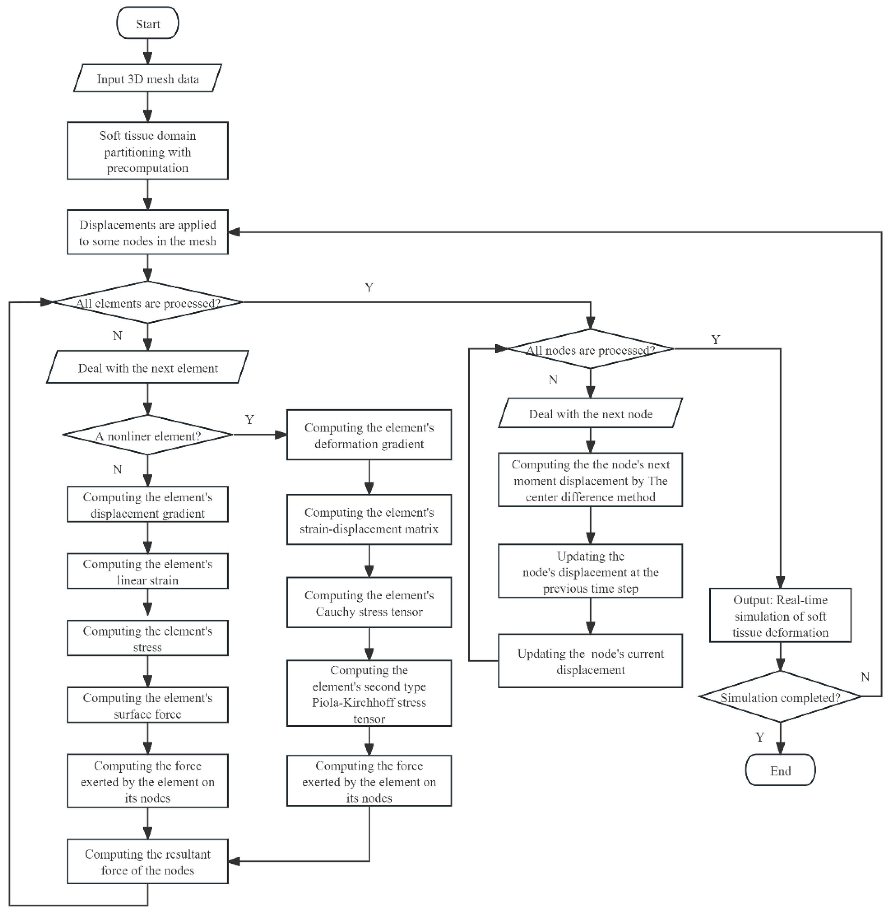
Figure 2.
Two tetrahedral subdivision strategies for cuboid elements. labels (a) and (b) denote two distinct subdivision types for cuboid elements. Both types are essential and must be employed in tandem. If only one subdivision type (e.g., Type (a)) is used exclusively, the edges along shared interfaces of adjacent cuboids will intersect rather than align, resulting in geometric incompatibility. However, a topologically consistent mesh can be achieved by ensuring that Type (a) elements exclusively share co-planar interfaces with Type (b) elements, and reciprocally, Type (b) elements only adjoin Type (a) elements through common planar boundaries. This alternating adjacency constraint guarantees mesh validity while preventing edge misalignment across neighboring elements.
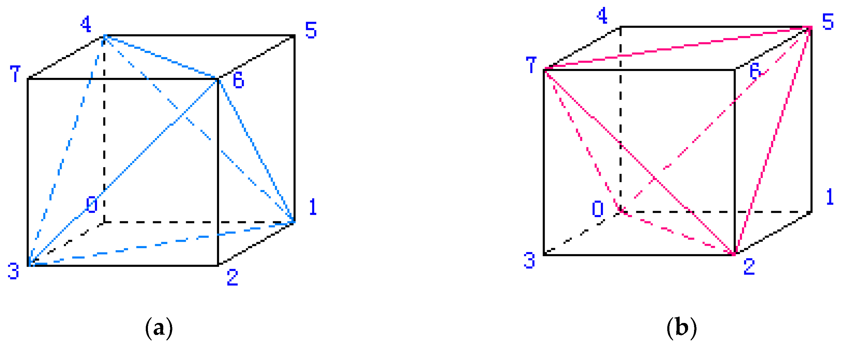
Figure 3.
A tetrahedral unit. This tetrahedral element is part of a simple three-dimensional mesh algorithmically generated, comprising 120 nodes and 300 such tetrahedral elements.
Figure 3.
A tetrahedral unit. This tetrahedral element is part of a simple three-dimensional mesh algorithmically generated, comprising 120 nodes and 300 such tetrahedral elements.
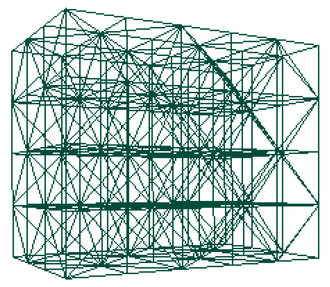
Figure 4.
The data structure of deformation model. The mesh comprises three interconnected lists (tetrahedra, surface triangles, vertex) with explicit associations. Each tetrahedron references four nodes via stored indices, enabling full node data retrieval (mass, position, forces, displacements). Connectivity is maintained through index pointers: tetrahedra reference nodes via indices acting as directional links to corresponding units, while triangles employ analogous indexing.
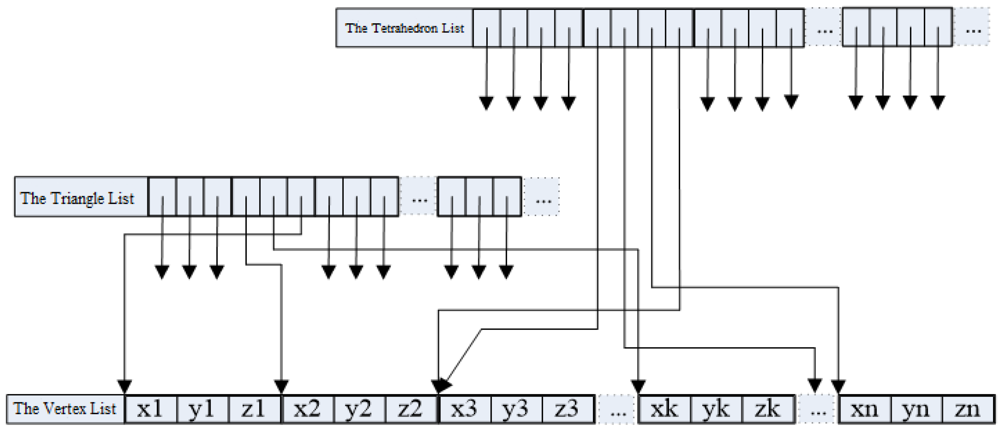
Figure 5.
A tetrahedron element.
Figure 6.
Direct Mass Matrix Lumping of a Bar Element. The total mass of the one-dimensional element, denoted as , is uniformly partitioned into two equal portions and assigned to its two nodal points.
Figure 6.
Direct Mass Matrix Lumping of a Bar Element. The total mass of the one-dimensional element, denoted as , is uniformly partitioned into two equal portions and assigned to its two nodal points.
Figure 7.
Direct Mass Lumping of Tetrahedral Element. Each node receives an equal mass portion , achieved by diagonalizing the mass matrix through shape function integration.
Figure 7.
Direct Mass Lumping of Tetrahedral Element. Each node receives an equal mass portion , achieved by diagonalizing the mass matrix through shape function integration.
Figure 8.
Central Difference Method for Calculating First-Order Displacement Derivatives. The first-order derivative at time t is computed using the central difference method.
Figure 8.
Central Difference Method for Calculating First-Order Displacement Derivatives. The first-order derivative at time t is computed using the central difference method.
Figure 9.
The operation effect of DHD-FEA model. (a) All elements are linear components. (b) All elements are nonlinear components. (c) The upper section of elements consists of linear components, while the lower section contains nonlinear components.
Figure 9.
The operation effect of DHD-FEA model. (a) All elements are linear components. (b) All elements are nonlinear components. (c) The upper section of elements consists of linear components, while the lower section contains nonlinear components.
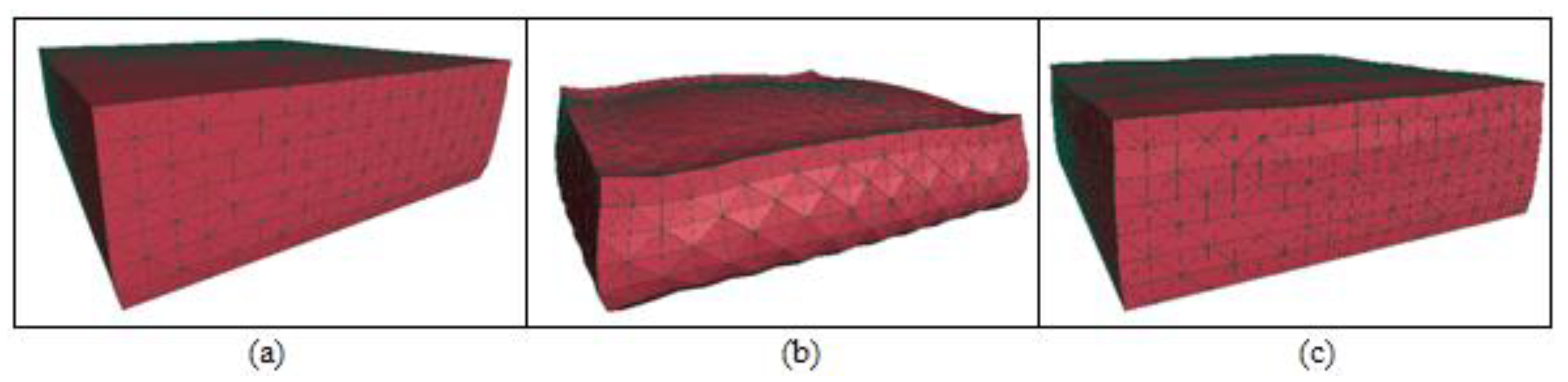
Figure 10.
Simulation scenario for error analysis of the DHD-FEA. The cuboid area is divided into a grid containing approximately 4000 tetrahedral elements. The bottom surface of the cuboid is fixed, while the top surface is the surgical interactive area. The upper elements of the cuboid are of non-linear type, with the edges represented in light color. The lower elements are of linear type, with the edges represented in dark color.
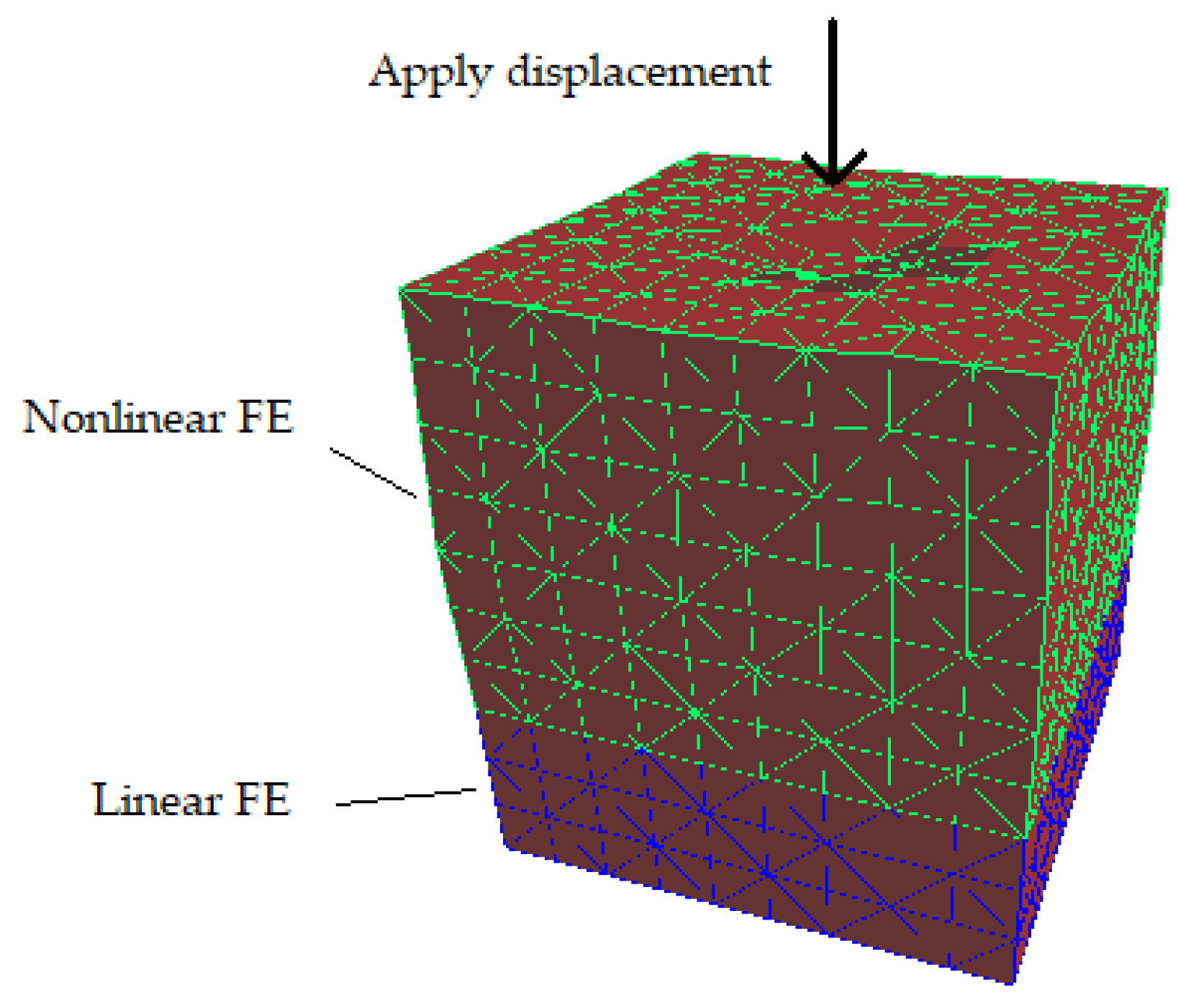

Table 1.
The algorithmic performance evaluation of DHD-FEA model.
| The proportion of linear elements | Frame rate |
|---|---|
| 0% | 22Hz |
| 10% | 24Hz |
| 20% | 28Hz |
| 30% | 32Hz |
| 40% | 34Hz |
| 50% | 40Hz |
1 As the proportion of linear elements in the DHD-FEA keeps increasing, the frame rate also gradually rises. This is mainly because a part of linear finite elements are mixed in the model, and the calculation efficiency of linear finite element elements is higher than that of nonlinear finite elements. When the proportion of linear elements is 0, all the elements in the model are nonlinear elements. At this time, the DHD-FEA is actually the TLED algorithm.
Table 2.
Error analysis of DHD-FEA model (1).
| The proportion of linear elements | Mean Error |
|---|---|
| 10% | 5.7% |
| 20% | 9.5% |
| 30% | 14.5% |
| 40% | 22.7% |
Table 3.
Error analysis of DHD-FEA model (2).
| The Proportion of Linear Elements | Mean Error |
|---|---|
| 10% | 5.8% |
| 20% | 9.8% |
| 30% | 15.1% |
| 40% | 23.7% |
Disclaimer/Publisher’s Note: The statements, opinions and data contained in all publications are solely those of the individual author(s) and contributor(s) and not of MDPI and/or the editor(s). MDPI and/or the editor(s) disclaim responsibility for any injury to people or property resulting from any ideas, methods, instructions or products referred to in the content. |
© 2025 by the authors. Licensee MDPI, Basel, Switzerland. This article is an open access article distributed under the terms and conditions of the Creative Commons Attribution (CC BY) license (http://creativecommons.org/licenses/by/4.0/).
Copyright: This open access article is published under a Creative Commons CC BY 4.0 license, which permit the free download, distribution, and reuse, provided that the author and preprint are cited in any reuse.


