
Submitted:
06 April 2025
Posted:
08 April 2025
You are already at the latest version
Abstract
In this work, we investigate the propagation and behavior of electromagnetic waves in traversable wormhole space-times influenced by topological defects. We focus on two specific scenarios: a Morris-Thorne-type traversable wormhole embedded in a space-time with a global monopole and another with a cosmic string. The primary objective is to examine how the wormhole geometry, combined with these topological defects, affects the dynamics and propagation of electromagnetic fields in curved space-time. To achieve this, we derive the Maxwell vacuum field equations in the context of curved geometries and solve them analytically, employing special functions to address the complexities introduced by the wormhole structure and defects. Our analysis highlights several key findings: the wormhole throat radius emerges as a critical parameter shaping the behavior of electromagnetic waves, while the presence of topological defects, such as the global monopole and cosmic string, introduces modifications to the electromagnetic fields. These modifications significantly alter the wave dynamics compared to those observed in Minkowski flat space-time, offering deeper insights into the interaction between electromagnetic phenomena and the geometry of curved space-times with topological defects.
Keywords:
Traversable wormholes
; Magnetic monopoles
; cosmic strings
; Maxwell’s Equations
; special functions
; Fuschian differential equations
1. Introduction
A symmetry-breaking phenomenon known as the decoupling of fundamental interactions is believed to have occurred during a phase transition in the early universe. This event, which marks a crucial moment in the history of the cosmos, is expected to give rise to topological defects-cosmic objects that are remnants of the symmetry-breaking process. Among the most studied of these defects are the “domain walls" [1], “cosmic strings" [2,3,4,5], and “global monopoles" (GMs) [6]. Although direct observational evidence for these defects remains elusive, the global monopole is considered the most promising candidate for future detection. This anticipation has driven a considerable amount of research, which has been documented in various studies and scientific literature [7,8,9,10,11,12,13,14].
Additionally, the behavior of global monopoles has been studied in the presence of other physical phenomena, such as dyons (particles that carry both electric and magnetic charges), magnetic flux, and scalar potentials. Precise solutions to the Klein-Gordon equation, which describes scalar fields, have been employed to understand the influence of GMs in various contexts. These studies have extended to the interaction of global monopoles with other fundamental forces, such as the electromagnetic and gravitational fields. Investigations into the Aharonov-Bohm effect [15,16,17,18], which describes the quantum mechanical interaction of charged particles with electromagnetic potentials, have also included global monopoles as a key component in understanding their potential physical implications. The exploration of global monopoles has not been confined to just scalar fields; the behavior of these objects in the presence of fermions has also garnered attention. In particular, the precise solutions to the Klein-Gordon and Dirac equations, which describe scalar and fermionic fields, respectively, have been examined in the context of GM. The study of these oscillators in relation to global monopoles provides important insights into the quantum mechanical properties of such defects, particularly with respect to energy levels and particle interactions in the presence of topological structures [19]. Moreover, the study of GMs is closely related to the broader field of topological defects in the universe, such as cosmic strings and domain walls, which have profound implications for the formation and evolution of the early universe. Despite the lack of experimental confirmation, the theoretical investigations into GMs continue to evolve, providing valuable information about the potential structure of the universe at its most fundamental level. It is expected that, as detection techniques improve, we may eventually observe these topological defects and validate many of the theoretical predictions that have emerged from decades of research.
Wormholes represent one of the many solutions permitted by general relativity (GR), and they have been extensively studied and analyzed in the literature [20,21]. These hypothetical structures are often envisioned as conduits that enable rapid connections between distant regions in spacetime or even between separate universes. Such properties have made wormholes a popular subject in theoretical physics. However, for wormholes to exist, they require the violation of the null energy condition, a fundamental constraint in GR. Wormholes are typically modeled as geometric structures with a tubular shape, which are asymptotically flat on both ends. Wormholes have been studied from a variety of perspectives, as reflected in numerous research papers [22,23,24,27,28,29,30,31,32,33,34,35]. Among the earliest and most fundamental wormhole solutions is the Ellis-Bronnikov wormhole [36,37]. This solution provides a simple yet effective framework for understanding the basic properties of wormholes in the context of general relativity. In addition, alternative theoretical models have emerged, with modified gravity theories exploring different aspects of wormhole physics without relying on exotic forms of matter, such as dark energy [38,39]. One such modified gravity theory is Born-Infeld gravity (EiBI), which is inspired by the work of Eddington [40]. EiBI gravity has been thoroughly examined due to its remarkable ability to avoid the formation of singularities, a characteristic that typically requires the introduction of exotic matter. The Morris-Thorne (or Ellis-Bronnikov) wormhole, developed within the framework of EiBI gravity, describes a spherically symmetric, static spacetime with a topological charge consistent with general relativity [41,42]. This solution was derived by incorporating the geometry of spacetime with the energy-momentum tensor corresponding to the region outside the global monopole (GM) core.
The study of the Morris-Thorne wormhole and similar solutions has been an active area of research, with numerous contributions advancing our understanding of their properties and implications. Notably, in 1988, Morris and his collaborator proposed an exact solution of the field equations involving exotic matter, which inherently violates energy conditions [22,23,24]. The space-time represents a wormhole metric and the line-element describing this wormhole is a spherically symmetric in the Schwarzschild coordinates given by
where is the redshift function and is called the shape function which determine the size of the throat of the wormhole. A few criteria is that this shape function must satisfy: (i) as , (ii) , where is the throat radius, and (iii) , where prime denotes ordinary derivative w. r. t. r, and (iv) . Numerous authors have been studied this wormhole space-times in general relativity as well as in modified gravity theories (see, for examples Refs. [25,26] and related references therein).
Building on the foundations of previous research, we aim to further explore the electromagnetic field equations within the context of Morris-Thorne-type wormhole space-time, specifically in the presence of a global monopole charge. Maxwell’s equations, which form the cornerstone of electrodynamics, serve as the guiding framework for our investigation [47,48,49,50,51]. Although these equations have been central to our understanding of electromagnetism for over a century, their interpretation and application continue to evolve as new theoretical developments emerge. The interplay between Maxwell’s electrodynamics and Einstein’s general theory of relativity has long been a subject of interest. Einstein’s work revealed a profound connection between the electromagnetic field and gravity, suggesting that gravity is not only influenced by mass and energy but can also interact with and be shaped by electromagnetic fields. This relationship, encapsulated in the Einstein-Maxwell equations, shows that the presence of a gravitational field can affect the behavior of the electromagnetic field. In turn, the electromagnetic field can influence the curvature of spacetime, reinforcing the idea that gravity can intensify or distort an existing electromagnetic field under certain conditions. This mutual influence between gravity and electromagnetism highlights the intricate dynamics between the fundamental forces, and it plays a crucial role in the quest for a Grand Unified Theory (GUT). Such a theory aims to merge all fundamental forces into a single, coherent framework, and the interaction between gravity and electromagnetism within the context of wormholes and global monopoles could provide essential insights into this larger goal. By studying the electromagnetic field equations in the background of Morris-Thorne-type wormhole space-time with global monopole charge, we seek to uncover new perspectives on the behavior of these fundamental forces under extreme conditions.
The relationship between space-time geometry and electromagnetic fields is fundamental in classical field theories, with gravity being one of the most important aspects. Electromagnetic fields, which carry energy and momentum, influence space-time geometry, and light propagates along null geodesics. This creates a critical connection between the causal structure of space-time and the propagation of electromagnetic fields. Given the close relationship between electrodynamics and the fundamental concept of causality in physics, this classical field theory plays a central role in our understanding of the universe. In the conventional particle paradigm, photons are massless particles responsible for carrying electromagnetic waves, which makes their connection to the light cone unique and allows for experimental exploration of null cones. Numerous studies have investigated various aspects of electromagnetism in curved space-time backgrounds. For instance, Cohen et al. [52] and other works have explored weak electromagnetic fields in rotating black holes [53], decoupling Maxwell’s equations in curved space-time [54], and electromagnetic fields in Petrov type-D and Kerr space-times [55], as well as in Kerr–NUT–(A)dS space-times [56,57], Myers-Perry geometry [58], higher-dimensional black hole space-times [59], and the Plebanski-Demianski metric [60]. It is important to note that Maxwell’s equations were the first relativistic field equations, and while the concept of the light cone originated in Minkowski space-time, it can also be derived from electrodynamics, and these equations possess a pre-metric formulation [61,62,63]. Additionally, studies such as Ref. [64] have investigated the electromagnetic field equations in Minkowski flat space, rotating flat space, and black hole space-times. In Ref. [65], the electromagnetic fields in curved space-time were explored, while in Ref. [66], the electromagnetic fields within a topological defect space-time, including both global monopoles and cosmic strings, were studied and Maxwell’s equations were solved. Similarly, in Ref. [67], the electromagnetic field tensor in the curved space-time of a spherically symmetric black hole accompanied by topological defects was examined, with the Schwarzschild black hole metric being employed to solve Maxwell’s vacuum equations. In Ref. [68], electromagnetic fields in the context of a traversable four-dimensional wormhole metric were analyzed, solving the Maxwell vacuum equations analytically in the presence of cosmic strings and global monopoles. Finally, in Ref. [69], the effects of a global monopole on electromagnetic fields in a curved space-time background under the framework of Eddington-inspired Born-Infeld (EiBI) gravity were explored, with the free Maxwell’s equations being solved analytically and their effects on electromagnetic wave propagation being analyzed.
In general relativity, Minikowski space-time is often extended to a more physically relevant, perhaps curved space-time when applied to electromagnetic. This evaluates how matter affects the universe’s space-time curvature. Considerable study on electromagnetic in curved areas has shown a clear connection between Einstein fields and Maxwell’s equations. The vector character of the electromagnetic field and the geometric framework created by general relativity result in this coupling, which is comparable to a sort of scattering where space-time curvature impacts the propagation of electromagnetic waves. The electromagnetic field equations in curved space-time may be represented as covariant versions, which can be used to formalise this complicated interaction[70,71,72,73].
And
where coma denotes ordinary/partial derivative w. r. t. argument.
It is important to represent the electromagnetic field tensor within a coordinate system before substituting the result into (3) to obtain the explicit version of the electromagnetic field equations. The electromagnetic field tensor in flat space-time with Cartesian coordinates has a unique structure: , . Although this representation has an explicit definition for Cartesian coordinates, it is less well-known in curvilinear coordinates inside flat space-times, and there aren’t as many explicit formulations for field equations and electromagnetic tensors. A more complete formulation becomes essential when searching for electromagnetic field equations in coordinate systems such as cylindrical or "Schwarzschild" coordinates.
In Ref. [69], we studied electromagnetic fields in a Klinkhamer-type traversable wormhole featuring a global monopole and subsequently considering a cosmic string and analyzed the radial solutions in detail. Building on this previous work, the current study focuses on another well-known traversable wormhole metric, featuring the topological defects as does in the previous work. This wormhole metric is called the Morris-Thorne-type traversable wormhole and we investigates the same phenomenon within this setup, incorporating a global monopole and then a cosmic string. We derive the Maxwell vacuum field equations and solve them analytically using special functions to address the mathematical complexities introduced by the wormhole structure and the topological defects. The analytical solutions are thoroughly examined to understand how the wormhole throat radius and the topological defects influence the propagation of electromagnetic waves in curved space-time. Moreover, it is shown that the results in the current study are fundamentally different from those results obtained in the previous work in Ref. [69], as we focus on a different wormhole geometry other than Klinkhamer-type wormhole. In addition, we demonstrate that the topological parameters, along with the wormhole throat radius, modify the present electromagnetic fields compared to flat Minkowski space. Our findings highlight the significant impact of the wormhole geometry and topological defects on the behavior of electromagnetic fields, providing new insights into the interaction between electromagnetic waves and the curvature and topology of space-time.
The structure of the paper is as follows: In Section 2, we present the electromagnetic field tensor in detail in the context of topologically charged Morris-Thorne-type wormhole and derive the corresponding Maxwell vacuum equations. In Section 3, we present the electromagnetic field tensor in the context of Morris-Thorne-type wormhole with a cosmic string and derive the corresponding Maxwell vacuum equations. We then solve these equations analytically using special functions and analyze the results. In Section 4, we provide our conclusions. Throughout the paper, we adopt units where .
2. Maxwell Equations in Morris-Thorne-type wormhole with a global monopole
In this part, we study Maxwell’s equation in curved space, specifically in the context of Morris-Thorne-type wormhole with topological defects. Therefore, we begin this section by writing the line element which is given by (setting red shift without loss of generality)
Here, where G is the Newtonian gravitational constant, being dimensionless volumetric mass density also called energy-scale of the symmetry breaking similar to GM [74]. Numerous authors have been studied wormhole space-times with global monopole charges in the context of quantum mechanical system (for example, see Refs. [43,44,45,46]). In the limit where , this metric reduced to a global monopole space-time. Recently, electromagnetic fields in this global monopole metric have been studied in [66].
The covariant and contravariant metric tensor for the above space-time will be
The tetrad vector related with metric tensor is given by the following relations
where is the Minkowski metric tensor, Greek indices run from 0 to 3 with and Latin indices . We derive the electromagnetic field tensor for the generic comoving observer in the considered curved space-time backgrounds as significant examples. The general comoving observer’s velocity is determined by ,
Using equations (6) and selecting the general comoving observer velocity (7) as , the coordinate tetrad for this metric is obtained as follows:
Noted that these tetrads can be immediately generated from the metric (4). In order to convert into spherical coordinates, we select the following and , the electromagnetic field tensor in non-coordinate basis is given by
Therefore, the electromagnetic field tensor in the background of a topologically charged Morris-Thorne-type wormhole by utilizing equation (39)-(9) in coordinate basis becomes
And it’s covariant form is given by,
From equation (2) and (10) we obtain the following vacuum electromagnetic field equations in the Morris-Thorne-type wormhole when we operate on a coordinate basis
for = 0,1,2,3, respectively.
Now, we attempt to find solution of the above electromagnetic field equations. So, differentiating Eq. (13) w. r. t. time t and using Eqs. (18)–(19) and finally then Eq. (12), we obtain the following differential equation in terms of as follows:
where we have used the following relation[75,76]
Here is the spherical harmonics, ℓ is the angular quantum number and m is the magnetic quantum number related by with .
Similarly, differentiating Eq. (17) w. r. t. time t and using Eqs. (14)–(15) and finally Eq. (16), we obtain the following equation for the magnetic field as follows:
Since the differential Eqs. (20) and (22) are of the same form, let’s consider the following ansatz for the electric and magnetic field components () given by
where is the frequency of the electromagnetic waves and is the radial function.
Substituting this solution (23) into the Eq. (20) and (22) results the same second-order differential equation given by
Below, we aim to solve the above differential equation (24) using different shape function form and analyze the result.
2.1. Analytical Solutions for Shape Function
In this case, we chose the following shape function form
where is the throat radius. This shape function satisfies the flare-out condition, namely , and as well other conditions. It is worth noting that numerous authors have studied the Morris-Thorne-type wormhole with this particular shape function in the context of general relativity as well as modified gravity theories (see Refs. [77,78,79] and the related references therein).
To solve the above equation, let us consider a transformation into the Eq. (26) and after some straightforward calculation results
where we defined
Therefore, the radial solution of Eq. (27) is the confluent Heun function and is given by
From the above expression, it is evident that the factors such as the global monopole characterized by the parameter , the wormhole throat radius characterized by the parameter , and the orbital quantum number ℓ including the frequency of the em waves alters the behavior of the radial solution.
In Figure 1, we show the radial solution from Eq. (32), varying parameters such as the global monopole parameter , the wormhole throat radius , and the frequency of the electromagnetic waves , while keeping the azimuthal quantum number fixed at . We observe that the radial solution exhibits a gradual increase with increasing s. However, in some panels, we observe that as one or more of the aforementioned parameters increases, the increasing trend of the radial solution shifts downward as well as upward.
In Ref. [69], we studied electromagnetic fields in topologically charged Klinkhamer traversable wormhole metric and analyzed the results. The radial solution is given by (changing notations , and in Eq. (67) in [69])
By comparing Eqs. (32) and (33), it is clear that the radial solutions are fundamentally different. This discrepancy arises because the current metric describes a Morris-Thorne-type traversable wormhole, while the previous one corresponds to a Klinkammer-type traversable wormhole. The key distinction lies in the geometric structure of these two types of wormholes, particularly in the presence of a global monopole, which affects the space-times in distinct ways. However, in the absence of the global monopole also, these results are completely different.
The complete solution of the radial electric magnetic field component is given by
where is the normalization constant.
From the expression in (34), it is clear that the global monopole parameter , the wormhole throat radius , and the frequency electromagnetic waves influence the behavior of the electromagnetic fields. As a result, the presence of these factors leads to modifications in the outcomes compared to the Minkowski flat space result previously obtained in [64].
In the limit where , topologically charged wormhole space-time (4) reduces to Ellis-Bronnikov-type wormhole metric [36,37]. Following the similar procedure, we find the radial component of the electric field (and magnetic field) as,
where is the normalization constant.
In Figure 2, we show the radial solution from Eq. (35), varying parameters such as the wormhole throat radius , and the frequency of the electromagnetic waves , while keeping the azimuthal quantum number fixed at . We observe that the radial solution exhibits a gradual increase with increasing s. This increasing trend shifts upward with increasing values of one or more of the aforementioned parameters.
2.2. Analytical Solutions for Shape Function,
In this case, we chose the following shape function form
where is the throat radius. It is worth noting that numerous authors have studied the Morris-Thorne-type wormhole with this particular shape function in the context of general relativity as well as modified gravity theories (see Refs. [77,78,79] and the related references therein).
Let us perform the transformation in the Eq. (37) and some algebraic calculation results
The above equation can be expressed in the standard 2nd-order Fuchsian ordinary differential equation form [82,83,84]:
where we defined
One can see that this equation (39) has three regular singular points at , and .
The presence of these singular points suggests the following transformation of as,
where p and q are determined to eliminate the singular terms at and .
Substituting (41) into the Eq. (39) and eliminate leading singularities near and gives us
And the resulting equation will be the following form:
which is the hypergeometric differential equation [80,81,85,86].
The solution to the above hypergeometric equation is:
where is the Gaussian hypergeometric function, and are constants of integration and other parameters are as follows:
Thus, the general solution therefore is given by
As we have shown that the parameters and c are related with the global monopole characterized by the parameter , the wormhole throat radius characterized by the parameter , and the orbital quantum number ℓ including the frequency of the em waves . Thus, the radial solution (79) of the electromagnetic fields gets influenced by these aforementioned parameters, and hence, alters the behavior.
Hence, the complete expression for the radial electric or magnetic field is given by
where is given in Eq. (46) and is the normalization constant.
3. Maxwell Equations in Morris-Thorne-type wormhole with a cosmic string
In this part, we study Maxwell’s equation in curved space, specifically in Morris-Thorne-type wormhole with a cosmic string. Therefore, we begin this section by writing the line element which is given by [87,88,89,90]
Here , the cosmic string parameter with being linear mass density of the string, and a is the wormhole throat radius. If we set , one will find a cosmic string space-time in the spherical coordinates system. Recently, electromagnetic fields in a cosmic string space-time background has been reported in [66].
The covariant and contravariant metric tensor for the above space-time will be
The coordinate tetrad for this metric tesnor (48) is as follows:
Therefore, the electromagnetic field tensor in the background of a Morris-Thorne-type wormhole by utilising equation (9) and (50) in coordinate basis becomes
And it’s covariant form is given by,
From equation (2) and (51), we obtain the following vacuum electromagnetic field equations:
for = 0,1,2,3, respectively.
Now, we attempt to find solutions of the electromagnetic field equations. Differentiating Eq. (54) w. r. t. time t and using Eqs. (59)–(60) and finally then Eq. (53), we obtain the following differential equation in terms of as follows:
Similarly, differentiating Eq. (58) w. r. t. time t and using Eqs. (55)–(56) and finally Eq. (57), we obtain the following equation for the magnetic field as follows:
where is the effective angular quantum number satisfying the following angular equation [66,67,68,69]
Since the differential Eqs. (61) and (62) are of the same form, let’s consider the following ansatz for the electric and magnetic field given by
where is the frequency of the electromagnetic waves and is the radial function.
As done in the earlier section, we choose different shape function for and solve the above differential equation (65).
3.1. Analytical Solutions for Shape Function,
Substituting the shape function form into the differential equation (65) results the following form:
where we set the following parameter
Following the procedure done in the previous section, we find
Thus, the radial solution R is the confluent Heun function given by
From the above expression, it is evident that the factors such as the cosmic string characterized by the parameter , the wormhole throat radius characterized by the parameter , and the magnetic quantum number m including the frequency of the em waves alters the behavior of the radial solution.
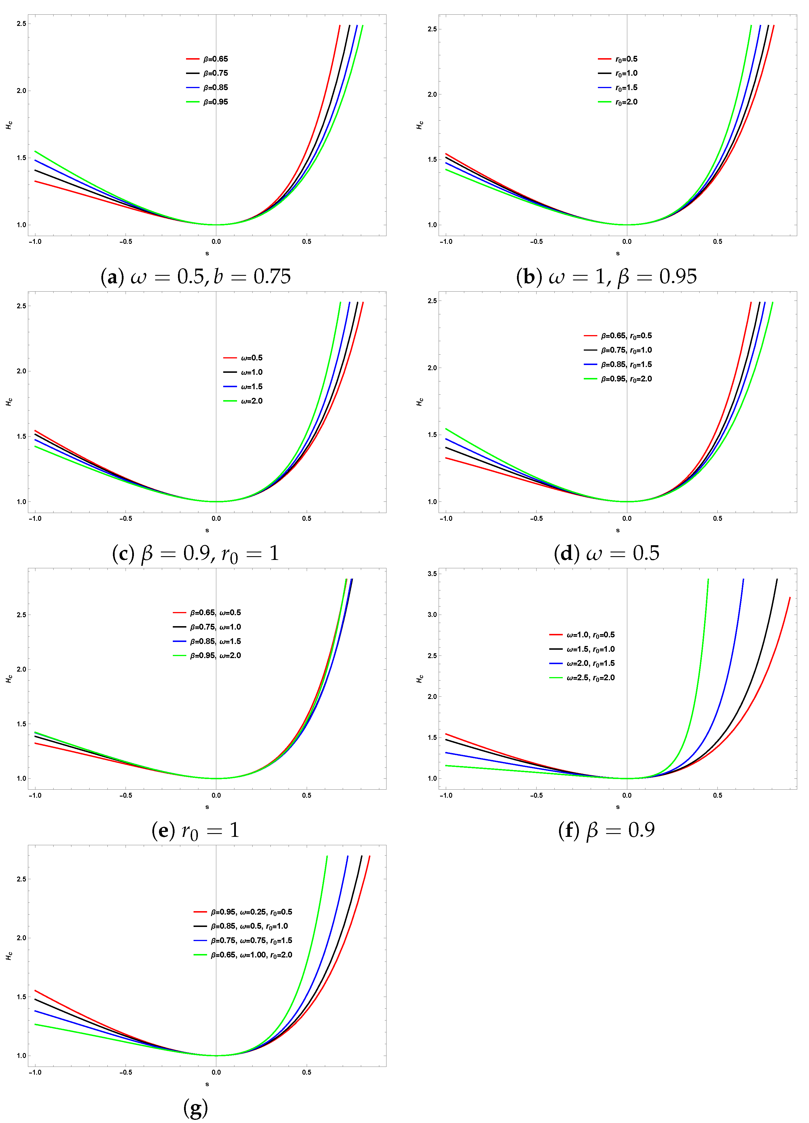
In Figure 3, we show the radial solution from Eq. (69), varying parameters such as the cosmic string parameter , the wormhole throat radius , and the frequency of the electromagnetic waves , while keeping the magnetic quantum number fixed at . We observe that the radial solution exhibits a gradual increase with increasing s. However, in some panels, we observe that as one or more of the aforementioned parameters increases, the increasing trend of the radial solution shifts downward as well as upward.
In Ref. [69], we studied electromagnetic fields in Klinkhamer-type traversable wormhole metric with cosmic string effects and analyzed the results. The radial solution is given by (changing notations , and in Eq. (31) in [69])
By comparing Eqs. (69) and (70), it is clear that these radial solutions are fundamentally different. This discrepancy arises because the current metric describes a Morris-Thorne-type traversable wormhole, while the previous one corresponds to a Klinkammer-type traversable wormhole, featuring a cosmic string in both wormhole metrics. The key distinction lies in the geometric structure of these two types of wormholes, particularly in the presence of a cosmic string, which affects the space-times in distinct ways. However, in the absence of the cosmic string also, one can easily show that these results are completely different.
Thus, the complete solution of the radial component of the electric or magnetic field is given by
where is the normalization constant.
In the limit when , the quantum number and , and therefore, the above result reduces to those obtained in the previous section given by Eq. (35).
3.2. Shape Function,
Substituting the shape function form into the equation (65) results the following differential equation:
Let us perform the transformation in the Eq. (72) and some algebraic calculation results
As done in the previous section, let us consider the following function of as,
where and are determined to eliminate the singular terms at and .
And the resulting equation will be the following form:
which is the Gaussian hypergeometric-type differential equation.
The solution to the above hypergeometric equation is:
where is the Gaussian hypergeometric function, and are constants of integration and other parameters are as follows:
Thus, the general solution becomes
As we have shown that the parameters and are related with the cosmic string characterized by the parameter , the wormhole throat radius characterized by the parameter , and the magnetic quantum number m including the frequency of the em waves . Thus, the radial solution (79) of the electromagnetic fields gets influenced by these aforementioned parameters, and hence, alters the behavior.
Hence, the complete expression for the radial electric or magnetic field is given by
where is given in Eq. (79) where is the normalization constant.
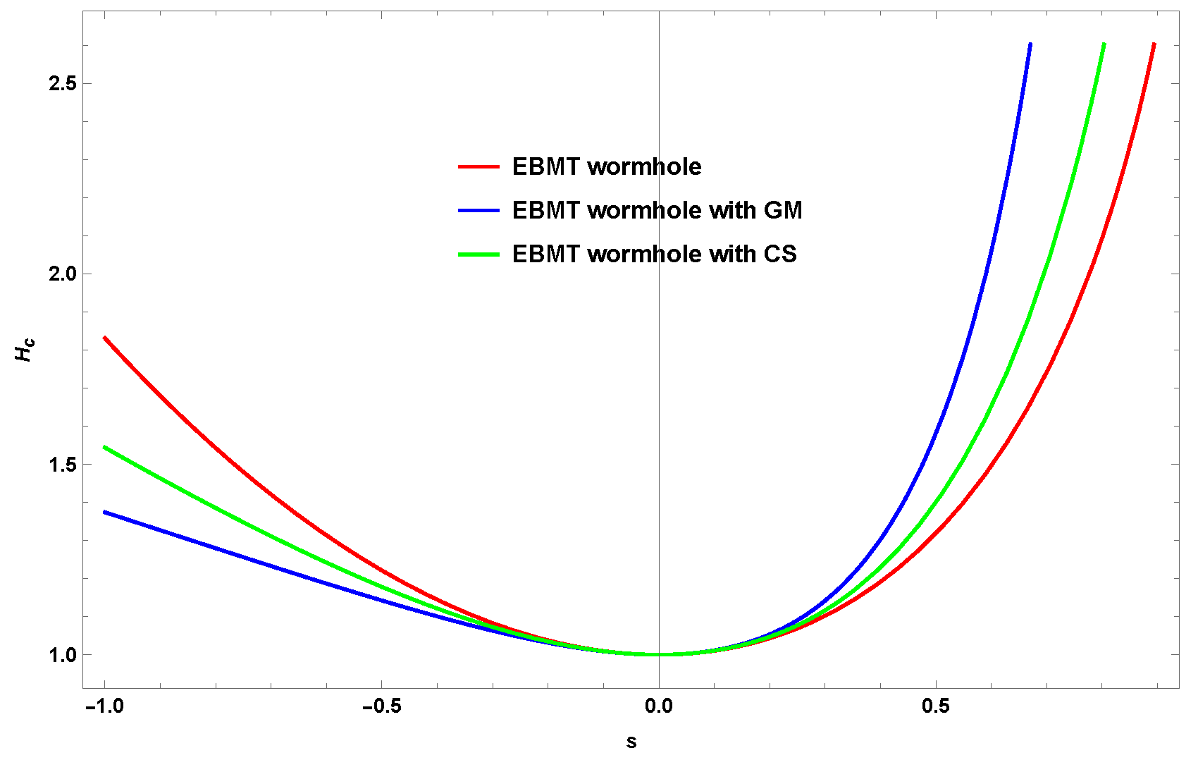
In Figure 4, we compare the radial solutions from Eq. (32), from Eq. (35), and from Eq. (69), both in the absence and presence of the global monopole and cosmic string effects. For this comparison, we fixed the wormhole throat radius at , the frequency of the electromagnetic waves at , the azimuthal quantum number at , the magnetic quantum number at , and set . This figure highlights the differences in how the presence of the global monopole and cosmic string, within a curved geometry, alters the behavior of the radial solutions of the electromagnetic fields compared to the case where these effects are absent.
4. Conclusions
This paper investigated the behavior of electromagnetic waves in Morris-Thorne-type traversable wormhole space-times embedded with topological defects, specifically focusing on a global monopole and a cosmic string. The primary aim was to derive and solve the Maxwell vacuum field equations in these curved geometries and analyze how the wormhole structure and the topological defects influence the propagation of electromagnetic fields.
Initially (Section 2), we studied a Morris-Thorne-type wormhole geometry incorporating a global monopole, characterized by the monopole parameter . Two forms of the wormhole shape function were considered: (i) and (ii) , where represents the wormhole throat radius. The Maxwell field equations were derived in this specific geometry, reduced to second-order differential equations, and solved analytically using special functions to address the complexities introduced by the curved space-time. Our analysis showed that both the monopole parameter and the throat radius significantly affect the behavior of electromagnetic waves, introducing distinct modifications to wave dynamics. These findings demonstrate how the unique curvature associated with the global monopole alters the propagation of electromagnetic fields compared to flat space-time.
In the second part of our study (Section 3), we extended the analysis to a Morris-Thorne-type wormhole geometry embedded with a cosmic string, characterized by the deficit angle parameter . Using the same forms of the shape function, we derived the Maxwell vacuum field equations in this curved geometry and followed a similar analytical approach to solve them. Our results indicated that the cosmic string parameter and the throat radius induce significant changes in the electromagnetic fields, leading to wave behavior distinct from that observed in Minkowski space-time. These effects highlight the influence of the cosmic string’s space-time topology on wave propagation.
Our findings emphasize the critical role of wormhole geometry and topological defects in shaping electromagnetic wave dynamics. The study underscores how parameters such as the global monopole and cosmic string introduce curvature and topological effects that profoundly influence electromagnetic wave behavior. The wormhole throat radius acts as a central geometric parameter, further modulating these effects. The implications of this work extend beyond theoretical interest, offering potential insights into astrophysical phenomena where such exotic space-time structures might exist. By showing how electromagnetic fields respond to the interplay between geometry and topology, this study contributes to the broader understanding of general relativity, wave propagation in curved space-times, and the observable effects of topological defects in the universe. These results pave the way for further exploration of physical processes in non-trivial geometries, deepening our comprehension of the relationship between space-time structure and field dynamics.
The discovery of the cosmic microwave background (CMB), predicted by Ralph et al. [91], remains a cornerstone of evidence for the Big Bang theory of the universe’s origin. While the CMB itself is predominantly smooth and uniform, it exhibits subtle anisotropies that can be precisely mapped using highly sensitive detectors. Ground-based and space-based experiments, such as NASA’s COBE (Cosmic Background Explorer), WMAP (Wilkinson Microwave Anisotropy Probe), and the ESA’s Planck spacecraft, have played a critical role in measuring these temperature fluctuations, enhancing our understanding of the early universe’s structure.
Similarly, the first direct detection of gravitational waves marked a groundbreaking achievement when a signal from the merger of two black holes was observed by the LIGO detectors [92], in collaboration with the VIRGO network. This discovery opened a new era in astrophysics, allowing us to probe the universe in an entirely new way. In more recent times, the Event Horizon Telescope’s imaging of the supermassive black hole at the center of the M87 galaxy has captured the scientific community’s attention and significantly advanced our understanding of black hole physics [93].
In a similar vein, we envision that, with the continued advancement of high-resolution radio, optical, and other specialized telescopes, detecting electromagnetic waves passing near exotic cosmic objects, such as wormholes, could become a reality in the near future. These observations would offer unprecedented insights into the nature of such objects, potentially unlocking new realms of understanding in both theoretical and observational astrophysics
Data Availability Statement
No new data generated or analyzed in this paper.
Acknowledgments
F.A. acknowledges the Inter University Centre for Astronomy and Astrophysics (IUCAA), Pune, India for granted visiting associateship.
Conflicts of Interest
Author(s) declare no such conflicts of interest.
References
- A. Vilenkin, Phys. Rep. 121, 263 (1985).
- A. Vilenkin and E. P. S. Shellard, Strings and Other Topological Defects, Cambrigde University Press, Cambridge (1994).
- A. Vilenkin, Phys. Lett. B 133, 177 (1983).
- W. A. Hiscock, Phys. Rev. D 31, 3288 (1985).
- B. Linet, Gen. Relativ. Gravit. 17, 1109 (1985).
- M. Barriola and A. Vilenkin, Phys. Rev. Lett. 63, 341 (1989).
- E. R. Bezerra de Mello and C. Furtado, Phys. Rev. D 56, 1345 (1997).
- E. R. Bezerra de Mello andF. C. Carvalho, Class. Quant. Grav. 18, 5455 (2001).
- E. R. Bezerra de Mello and F. C. Carvalho, Class. Quant. Grav. 18, 1637 (2001).
- E. R. Bezerra de Mello, Class. Quant. Grav. 19, 5141 (2002).
- E. R. Bezerra de Mello, J. Spinelly and U. Freitas, Phys. Rev. D 66, 024018 (2002).
- E. R. Bezerra de Mello and A. A. Saharian, Class. Quant. Grav. 29, 135007 (2012).
- T. R. P. Caramˆes, J. C. Fabris, E. R. Bezerra de Mello and H. Belich, Eur. Phys. J. C 77, 496 (2017).
- E. R. Bezerra de Mello, Braz. J. Phys. 31, 211 (2001).
- A. L. Cavalcanti de Oliveira and E.R. Bezerra de Mello, Class. Quant. Grav. 23, 5249 (2006).
- A. Boumali and H. Aounallah, Adv. High Energy Phys. 2018, 1031763 (2018).
- H. Aounallah and A. Boumali, Phys. Part. Nucl. Lett. 16, 195, (2019).
- A. Boumali and H. Aounallah, Rev. Mex. Fis. 66, 192 (2020).
- E. A. F. Braganca, R. L. L. Vitoria, H. Belich and E. R. B. de Mello, Eur. Phys. J. C 80, 206 (2020).
- L. Flamm, Physikalische Zeitschrift 17, 448 (1916).
- A. Einstein and N. Rosen, Phys. Rev. 48, 73 (1935).
- M. S. Morris and K. S. Thorne, Amer. J. Phys. 56, 395 (1988).
- M. S. Morris, K. S. Thorne and U. Yurtsever, Phys. Rev. Lett. 61, 1446 (1988).
- M. Visser, Lorentzian Wormholes: From Einstein to Hawking, AIP Press, New York (1995).
- A. Chanda, S. Dey, and B. C. Paul, Gen. Relativ. Gravit. 53, 78 (2021).
- C. C. Chalavadi and V. Venkatesha, EPL 146, 39001 (2024).
- S. W. Hawking, Phys. Rev. D 46, 603 (1992).
- J. L. Friedmann, K. Schleich and D. N. Witt, Phys. Rev. Lett. 71, 1486 (1993).
- V. Frolov and I. D. Novikov, Phys. Rev. D 48, 1607 (1993).
- J. P. S. Lemos and F. S. N. Lobo, Phys. Rev. D 78, 044030 (2008).
- S.-W. Kim and H. Lee, Phys. Rev. D 63, 064014 (2001).
- F. Rahaman, P. K. F. Kuhfittig, M. Kalam, A. A. Usmani and S. Ray, Class. Quant. Grav. 28, 155021 (2011).
- T. A. Roman, Phys. Rev. D 47, 1370 (1993).
- G. C. Samanta and N. Godani, Eur. Phys. J. C 79, 623 (2019).
- J. Sadeghi, M. Shokri, S. Noori Gashti, B. Pourhassan and P. Rudra, Int. J Mod. Phys. D 31, 2250019 (2022).
- H. G. Ellis, J. Math. Phys., 14, 104 (1973).
- K. A. Bronnikov, Acta Phys. Pol. B 4, 251 (1973).
- S. Nojiri and S. D. Odintsov, Int. J. Geom. Meth. Mod. Phys. 4, 115 (2007).
- P. Brax, Rep. Prog. Phys. 81, 1 (2018).
- M. Ba˜nados and P. G. Ferreira, Phys. Rev. Lett. 105, 011101 (2010).
- J. R.Nascimento, G. J. Olmo, A. Yu. Petrov, P. J. Porfirio, A. R. Soares, Phys. Rev. D 99, 064053 (2019).
- R. D. Lambaga and H. S. Ramadhan, Eur. Phys. J. C 78, 436 (2018).
- A. R. Soares, R. L. L. Vitoria and H. Aounallah, Eur. Phys. J. Plus 136, 966 (2021).
- H. Aounallah, A. R. Soares and R. L. L.Vitória, Eur. Phys. J. C 80, 447 (2020).
- F. Ahmed, H. Aounallah and P. Rudra, Indian J Phys (2024). [CrossRef]
- A. Moussa, H. Aounallah, P. Rudra and F. Ahmed, Int. J Geom. Meths Mod. Phys. 20, 2350102 (2023).
- F. Gronwald, F.W. Hehl and J. Nitsch, [physics.class-ph] (2005). arXiv:physics/0506219.
- F. W. Hehl and Y. N. Obukhov, Chapter: Spacetime Metric from Local and Linear Electrodynamics: A New Axiomatic Scheme, Lect. Notes Phys. 702, 163 (2006).
- F. W. Hehl and Y. N. Obukhov, Chapter: How Does the Electromagnetic Field Couple to Gravity, in Particular to Metric, Nonmetricity, Torsion, and Curvature?, Lect. Notes Phys. 562, 479 (2001).
- F. W. Hehl, Ann. Phys. (Berlin) 520, 691 (2008).
- F. W. Hehl and Y. N. Obukhov, Gen. Relativ. Grav. 37, 733 (2005).
- J. M. Cohen and L. S. Kegeles, Phys. Rev. D 10, 1070 (1974).
- E. D. Fackerell and J. R. Ipser, Phys. Rev. D 5, 2455 (1972).
- Y. V. Taistra, Proceedings of the 22nd Annual Conference of Doctoral Students-WDS 2013 J. Šafránková (Eds.), Contributed Papers: Part III–Physics, Matfyzpress, Prague pp. 29–32(2013).
- V. O. Pelykh and Y. V. Taistra, J. Math. Sci. 229, 162 (2018).
- P. Krtous, V. P. Frolov and D. Kubiznak, Nucl. Phys. B 934, 7 (2018).
- I. Kolar and P. Krtous, Phys. Rev. D 91, 124045 (2015).
- O. Lunin, JHEP 12, 138 (2017).
- P. Krtous, Phys. Rev. D 76, 084035 (2007).
- V. P. Frolov, P. Krtous and D. Kubiznak, Phys. Rev. D 97, 101701(R) (2018).
- C. Lammerzahl and F. W. Hehl, Phys. Rev. D 70, 105022 (2004).
- Y. Itin and F. W. Hehl, Ann. Phys. (NY) 312, 60 (2004).
- F. W. Hehl and Y. N. Obukhov, Found. Phys. 35, 2007 (2005).
- H. Ramezani-Aval, Indian-J Phys. 96, 4347 (2022).
- C. G. Tsagas, Class. Quantum Grav. 22, 393 (2005).
- M. G. Kurbah and F. Ahmed, Indian-J Phys. (2024). [CrossRef]
- M. G. Kurbah and F. Ahmed, Mod. Phys. Lett. A 39, 2450172 (2024).
- M. G. Kurbah and F. Ahmed, Eur. Phys. J. C 84, 903 (2024).
- M. G. Kurbah and F. Ahmed, Eur. Phys. J. C 84, 1205 (2024).
- L. D. Landau and E. M. Lifshitz, The classical theory of fields, Pergamon Press (1975).
- F. W. Hehl and Y. N. Obukhov, Foundations of Classical Electrodynamics, Birkhäuser Boston, MA (2023).
- J. A. Stratton, Electromagnetic theory, Moskva-Leningrad (1948).
- V. Novacu, Introduction to electrodynamics, Moskva (1963).
- E. R. Bezerra de Mello, Braz. J. Phys. 31, 211 (2001).
- M. Abramowitz and I. A. Stegun, Handbook of Mathematical Functions with Formulas, Graphs, and Mathematical Tables, New York: Dover (1972).
- G. B. Arfken, H. J. Weber and F. E. Harris, Mathematical Methods for Physicists, Elsevier (2012).
- F. S. N. Lobo, Class. Quantum Gravit. 25, 175006 (2008).
- F. Ahmed, Sci. Rep. 13, 12953 (2023).
- J. Goswami, H. Rahman, R. Sikdar, R. Parvin and F. Ahmed, Eur. Phys. J. C 84, 1037 (2024).
- A. Ronveaux, Heun’s Differential Equations, Oxford University Press, Oxford (1995).
- S. Y. Slavyanov and W. Lay, Special Functions: A Unified Theory Based in Singularities, Oxford University Press, New York (2000).
- L. Fuchs, J. Reine Angew. Math. 66, 121 (1866).
- L. Fuchs, J. Reine Angew. Math. 68, 354 (1868).
- K. Heun, Math. Ann. 33, 161 (1889).
- W. N. Bailey, Generalised Hypergeometric Series (Cambridge tracts in mathematics and mathematical physics No. 32), Cambridge University Press, Cambridge, England (1935).
- P. M. Morse and H. Feshbach, Methods of Theoretical Physics, Part I (International Series in Pure and Applied Physics), New York: McGraw-Hill (1953).
- F. Ahmed, Indian-J. Phys. 98, 3601 (2024).
- F. Ahmed, EPL 142, 39002 (2023).
- F. Ahmed, Few-Body Syst 64, 80 (2023).
- F. Ahmed, Int. J. Mod. Phys. A 38, 2350178 (2023).
- R. A. Alpher, R. C. Herman, Nature 162, 774 (1948).
- The LIGO Scientific Collaboration, et al., Phys. Rev. Lett. 116, 061102 (2016).
- Event Horizon Telescope Collaboration, et al., ApJL 930, L12 (2022).
Figure 1.
The radial solution given in Eq. (32) for various values of parameters, such as the global monopole , the throat radius , frequency of the em waves keeping the orbital quantum number fixed.
Figure 1.
The radial solution given in Eq. (32) for various values of parameters, such as the global monopole , the throat radius , frequency of the em waves keeping the orbital quantum number fixed.
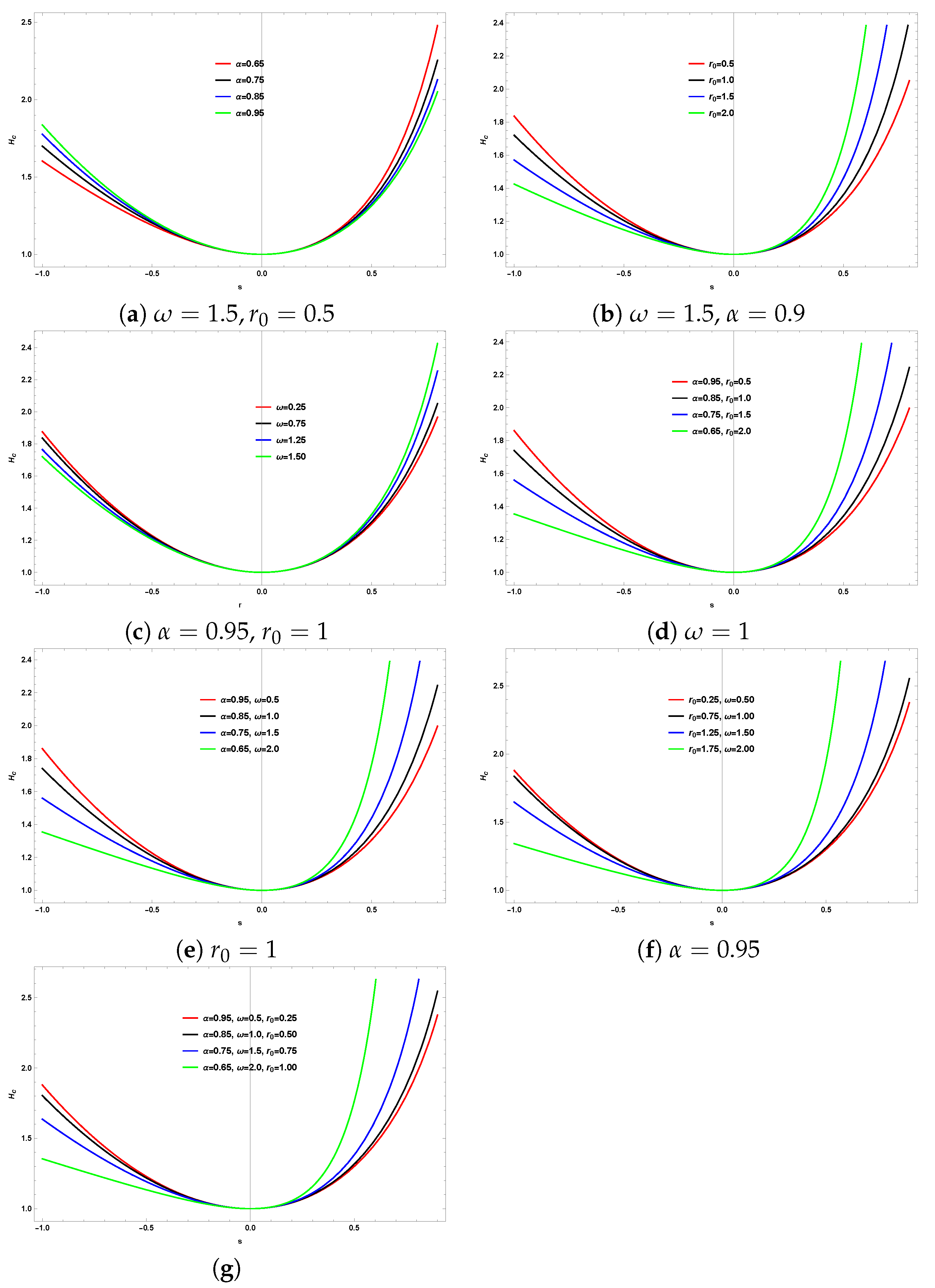
Figure 2.
The radial solution given in Eq. (35) for various values of parameters, such as the throat radius , frequency of the em waves , and the orbital quantum number ℓ.
Figure 2.
The radial solution given in Eq. (35) for various values of parameters, such as the throat radius , frequency of the em waves , and the orbital quantum number ℓ.
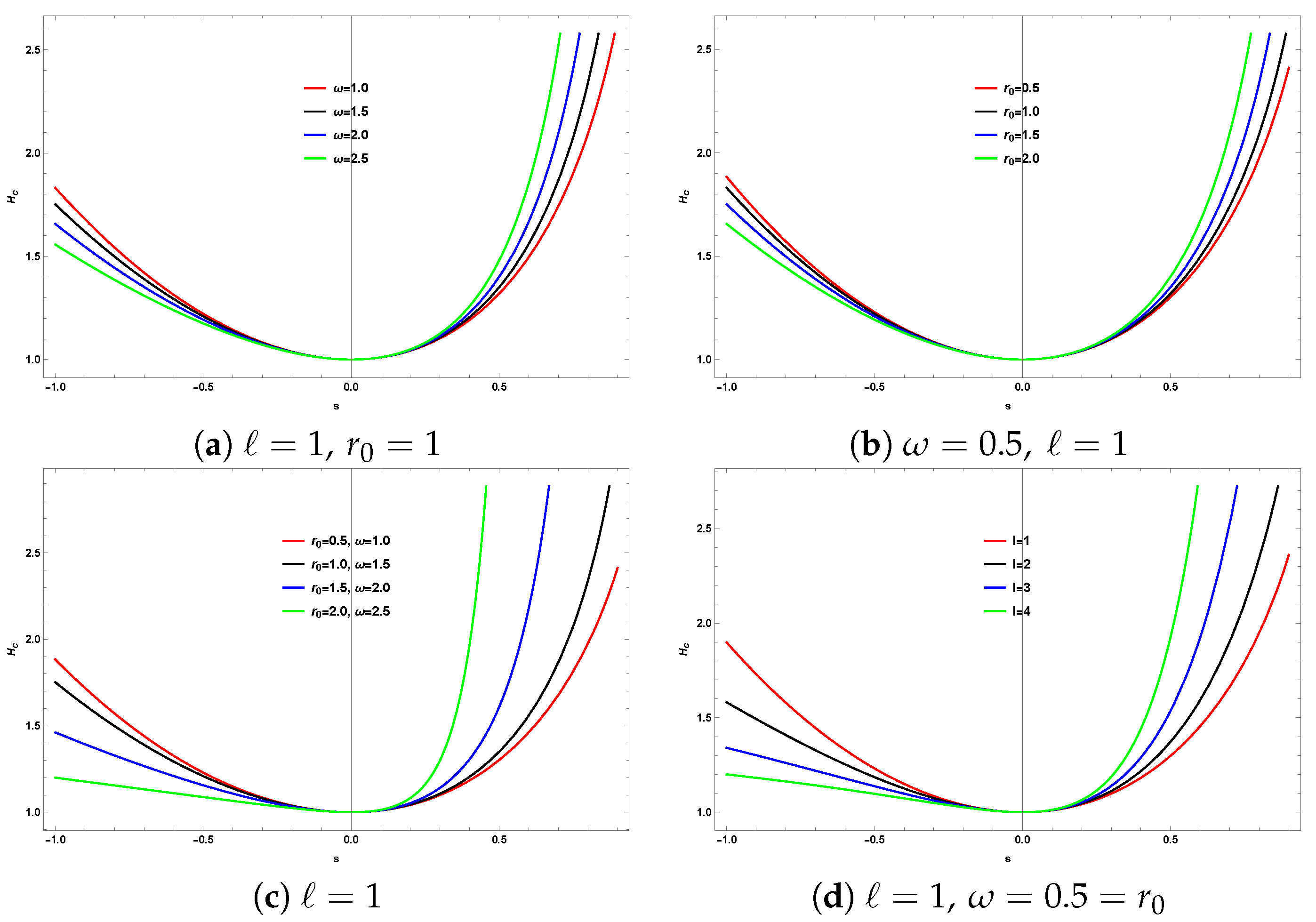
Figure 3.
The radial solution given in Eq. (32) for various values of parameters, such as the global monopole , the throat radius , frequency of the em waves keeping the orbital quantum number fixed.
Figure 3.
The radial solution given in Eq. (32) for various values of parameters, such as the global monopole , the throat radius , frequency of the em waves keeping the orbital quantum number fixed.
Disclaimer/Publisher’s Note: The statements, opinions and data contained in all publications are solely those of the individual author(s) and contributor(s) and not of MDPI and/or the editor(s). MDPI and/or the editor(s) disclaim responsibility for any injury to people or property resulting from any ideas, methods, instructions or products referred to in the content. |
© 2025 by the authors. Licensee MDPI, Basel, Switzerland. This article is an open access article distributed under the terms and conditions of the Creative Commons Attribution (CC BY) license (http://creativecommons.org/licenses/by/4.0/).
Copyright: This open access article is published under a Creative Commons CC BY 4.0 license, which permit the free download, distribution, and reuse, provided that the author and preprint are cited in any reuse.


