

Submitted:
04 July 2026
Posted:
06 July 2026
You are already at the latest version
Abstract
We present Furones, a linear-time candidate-comparison algorithm for the Minimum Dominating Set (MDS) problem on undirected graphs. The algorithm (version v0.3.8) applies a TSCC-style pendant cascade, solves the reduced instance by a Baker-style routine used only as a validated candidate generator, and compares the lifted candidate against several original-graph candidates: closed-degree coverage, witness sweeps, order ownership, seed completion, a Salvador-style auxiliary, a max-cut double-cover auxiliary, and reverse-delete scans. We prove two unconditional guarantees. First, every normal return is a valid dominating set. Second, because the portfolio contains the dynamic greedy maximum-coverage dominator, every returned set D satisfies |D| ≤ H(∆ + 1) γ(G) ≤ (1 + ln(∆ + 1)) γ(G), where ∆ is the maximum degree and H(k) is the k-th harmonic number; this is a constant factor on bounded-degree graphs and sub-logarithmic in n for sub-polynomial degree. We also record the near-threshold ratio hypothesis that Furones meets ratio max{4, ln n} on all graphs; proving it would imply P = NP. The hypothesis is already proved for all graphs with ∆ ≤ √n/e. Exact benchmarks on 11,000 small instances with exhaustive optimum certificates record zero violations of the conjectured bound.
Keywords:
dominating set
; approximation algorithm
; linear-time algorithm
; Baker’s technique
; graph optimization
; P versus NP
MSC: 05C69; 68Q25; 68W25; 90C27
1. Introduction
The Minimum Dominating Set problem asks, for an undirected graph , for the smallest set such that every vertex of G is either in D or adjacent to a vertex in D. We write for this minimum size. Dominating Set is one of the standard NP-hard graph optimisation problems, and it appears in network monitoring, facility placement, wireless-network design, and combinatorial covering models.
The approximation landscape is substantially harsher than for Minimum Vertex Cover. Vertex Cover admits a classical polynomial-time factor-2 approximation, whereas Dominating Set inherits logarithmic hardness from Set Cover. The greedy Set Cover analysis of Johnson, Lovász, and Chvátal gives a positive guarantee in terms of the maximum degree [1,2,3], and this analysis is tight [4]. On the negative side, the results of Feige and of Raz–Safra, sharpened to the optimal threshold by Dinur and Steurer, imply that no polynomial-time algorithm approximates general Minimum Dominating Set to within any factor that is in the number of vertices n unless ; in particular, a polynomial-time constant-factor approximation would be a -level breakthrough [5,6,7]. The two frontiers are not in conflict: is sub-logarithmic in n exactly when , and it recovers the frontier only in the worst case . Therefore, any claim that crosses the -in-n hardness frontier must be stated with its complexity-theoretic consequence explicitly on the page.
Scope and contribution. This paper presents the Furones solver for Dominating Set. The claims are separated into the parts that are presently proved by the implementation and the part that would settle a major complexity question:
- 1.
- A code-faithful description of Furones v0.3.8 (Algorithm 3), combining TSCC-style reductions, a Baker-style reduced-instance path, and multiple independent linear candidate generators on the original working graph.
- 2.
- A feasibility theorem (Theorem 1) showing that every normal return is a dominating set of the original input graph. The proof uses the local reduction rules, the explicit reduction-soundness lemmas of Section 3.6, domination-preserving pruning, and the final NetworkX domination validation.
- 3.
- An unconditional, degree-parameterised approximation theorem (Theorem 3). The portfolio includes the standard dynamic greedy maximum-coverage dominator (Algorithm 4), so the returned set obeys . For graphs with sub-polynomial maximum degree this is a sub-logarithmic-in-n guarantee, and for bounded-degree graphs it is a constant-factor guarantee (Corollary 3); the result is consistent with the hardness frontier precisely because may be .
- 4.
- A near-threshold ratio hypothesis (Hypothesis 1): Furones meets the ratio on every finite graph. We prove its consequence (Theorem 4): since sits below the optimal inapproximability threshold, establishing the hypothesis would imply . We also give evidence (Proposition 1): the hypothesis is already a theorem for all graphs of maximum degree , so only the high-degree regime is conjectural. This is the genuine boundary between what Theorem 3 proves unconditionally and what would settle a major complexity question.
- 5.
- A runtime analysis (Theorem 2) establishing a linear profile for fixed parameters, while making explicit that the hidden constant is large: the implementation runs many graph scans, several reverse-delete orders, fixed seed-completion passes, a Salvador auxiliary path, reduction/lift work, pruning, and final validation.
- 6.
- An exact CAR-style experimental study covering a 1000-instance ratio/ablation benchmark, a 1000-instance high-degree probe, and a -instance adversarial stress test, all with exact domination numbers computed by exhaustive search. These experiments measure the observed finite-benchmark ratio and each strategy’s valid size, optimum-attainment percentage, and min-attainment percentage; they are exact finite evidence, not a universal approximation proof.
The remainder of the paper is organized as follows. Section 2 records research data and implementation metadata. Section 3 describes Furones and its candidate families. Section 4 states the reduction-soundness lemmas and proves feasibility. Section 5 gives a per-subroutine worst-case analysis establishing the linear-time profile with its large-constant caveat. Section 6 proves the unconditional degree-parameterised approximation theorem and then states the constant-ratio hypothesis and the implication. Section 7 reports the exact CAR benchmarks, including the per-strategy candidate-comparison table, the high-degree probe, and the adversarial stress test. Section 8 discusses how to interpret the evidence, and Section 9 concludes.
2. Research Data and Implementation
The implementation studied here is the Python package Furones: Approximate Dominating Set Solver, available through the Python Package Index and maintained in a public repository [8]. Table 1 summarises the released package metadata.
Reproducibility Bundle
The repository contains the implementation, command-line entry points, targeted regression scripts, and the CAR-style exact benchmarks used in Section 7. Reproducing any CAR study requires installing the released package first with pip install furones (v0.3.8); each rerun script then imports from furones.algorithm import find_dominating_set, so the reported numbers reflect the installed solver. The repository’s car/ folder contains run_integrity_measurements.py, CAR.furones-v0.3.8.json, CAR-001-ratio-constant.json, CAR-002-strategy-ablation.json, run_high_degree_experiment.py, CAR-003-high-degree.json, run_adversarial_experiment.py, CAR-004-adversarial.json, family_summary.csv, and the per-instance CSV outputs. The exact CAR benchmark uses 1000 deterministic small graphs with at most 14 vertices and computes by exhaustive search before comparing Furones to the optimum.
3. The Furones Algorithm
3.1. Overview
Given an undirected NetworkX graph and an approximation parameter , Furones first handles trivial cases, removes self-loops, separates isolated vertices, and builds candidates on the non-isolated working graph H. Since Dominating Set does not have a general maximal-matching safety net analogous to the standard Vertex Cover factor-2 routine, the algorithm uses a portfolio: every candidate is pruned, directly checked for domination, and the smallest valid candidate is returned.
Input Conventions and Preprocessing
The public routine requires an undirected NetworkX graph. Empty graphs return ∅. Edgeless graphs return all vertices, since every isolated vertex must dominate itself. Self-loops are removed because they do not change domination in a simple undirected graph. Isolated vertices are stored and reinserted at the end, since each isolated vertex is mandatory in every dominating set.
Furones then computes the following candidate families:
- — Lifted TSCC/Baker candidate.
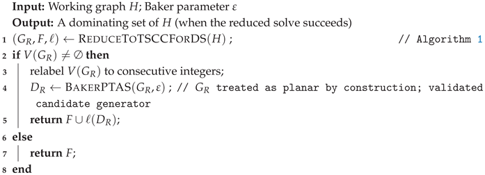
- Apply the TSCC-style isolated/pendant cascade, solve the reduced instance with a Baker-style routine [11] (used only as a validated candidate generator), and lift the reduced solution back to the original labels as .
- — Greedy maximum coverage.
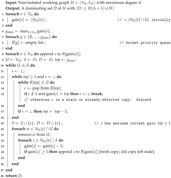
- Repeatedly select a vertex whose closed neighbourhood covers the largest number of still-undominated vertices, updating residual coverage after each selection, until every vertex of H is dominated (Algorithm 4). This is the classical Set Cover greedy [1,2,3] specialised to closed neighbourhoods; it is the candidate that certifies the unconditional guarantee of Theorem 3, and its presence is what makes that guarantee code-faithful.
- — Closed-degree coverage.
- Bucket vertices by their initial closed degree and scan once from largest to smallest, selecting a vertex only when it dominates a still-undominated vertex. The ordering is computed once and not re-evaluated, so is a cheaper static surrogate for that trades the worst-case guarantee for a single linear pass.
- — Low-degree witnesses.
- Score each vertex by the number of degree-one and degree-two witnesses in its closed neighbourhood, then run the same coverage-and-prune sweep.
- — Medium-degree witnesses.
- Score responsibility over moderate-degree witnesses, downweighting high-degree selector or booster noise that can mislead raw degree.
- — Order ownership.
- Assign moderate-degree witnesses to deterministic high-degree owners under early and late order rules, then sweep by ownership score.
- — Seed and complete.
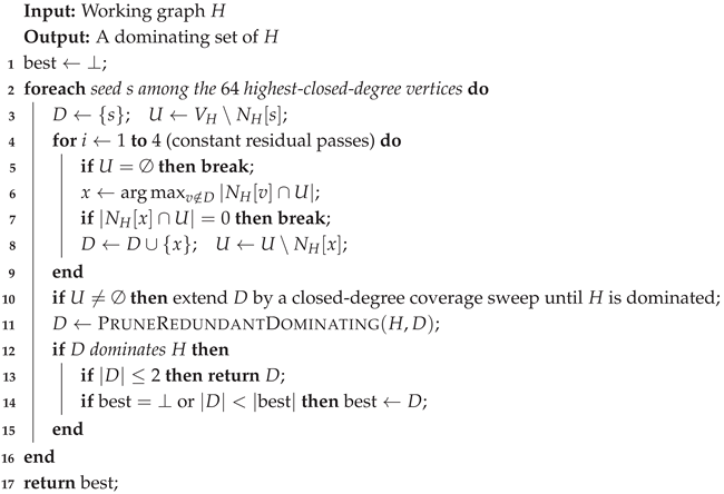
- Try a fixed number of high-coverage seeds, complete each residual by a constant number of complement passes, and keep the smallest valid completion.
- — Salvador-style auxiliary.
- Build the planar bipartite oriented-incidence auxiliary graph from the Salvador v0.0.3 gadget, change the auxiliary objective from weighted Vertex Cover to weighted Dominating Set, solve a Baker-style auxiliary candidate, decode selected incidence nodes, and validate the decoded set on the original graph.
- — Max-cut double-cover.
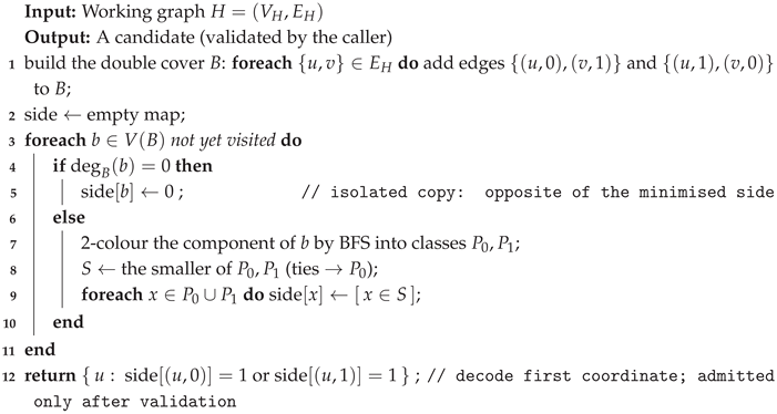
- Build the bipartite double cover , in which each vertex v has copies and each edge contributes the crossing edges and ; compute an exact maximum cut of that minimises one side (Algorithm 10), and decode the first coordinates of the minimised side as an original-graph candidate, validated on H (Section 3.5).
- — Reverse delete.
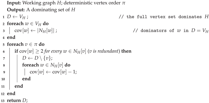
- Start from all vertices and process a constant number of deterministic orders, deleting a vertex only when domination remains valid.
The final answer is
with isolated vertices reinserted. Because validity is checked after pruning and after reinserting isolates, the algorithm never relies on a candidate generator being correct in isolation.
3.2. TSCC Pendant Gadget
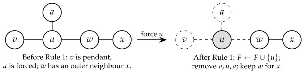
The local rule used by the reduction is the Dominating Set pendant rule. If v is pendant in the current working graph H and u is its unique H-neighbour, then replacing v by u preserves domination of the local structure. The v0.3.8 implementation is selective: it removes v, u, and neighbours of u that have no outer responsibility, while keeping neighbours that still have edges outside .
Figure 1.
Selective pendant gadget for the v0.3.8 TSCC-style Dominating Set reduction. Dashed vertices and edges are removed from the working graph; the gray vertex is inserted into the forced set F; the outer vertex w is kept because it still has a neighbour x outside .
Figure 1.
Selective pendant gadget for the v0.3.8 TSCC-style Dominating Set reduction. Dashed vertices and edges are removed from the working graph; the gray vertex is inserted into the forced set F; the outer vertex w is kept because it still has a neighbour x outside .
3.3. Pipeline
Figure 2 shows the whole solver pipeline. The important design choice is that the original-graph linear candidates are not merely fallbacks after the reduced-instance path. They are computed early, can return immediately when they find a valid set of size at most two, and are compared again against the lifted TSCC/Baker candidate after pruning.
3.4. Salvador-Style Auxiliary Candidate
The Salvador v0.0.3 construction maps an original edge to incidence vertices and and a forcing edge between them. Furones keeps this planar bipartite gadget but changes the objective: the auxiliary graph is treated as a weighted planar-bipartite Dominating Set instance, not as a weighted Vertex Cover instance. The decoded original-graph set is admitted only if it dominates the original graph after pruning.
Figure 3.
Salvador-style bipartite planar reduction gadget. In Salvador v0.0.3 this gadget is used for weighted Vertex Cover; in Furones v0.3.8 the same planar bipartite auxiliary graph is used as a weighted Dominating Set candidate and decoded only after validation.
Figure 3.
Salvador-style bipartite planar reduction gadget. In Salvador v0.0.3 this gadget is used for weighted Vertex Cover; in Furones v0.3.8 the same planar bipartite auxiliary graph is used as a weighted Dominating Set candidate and decoded only after validation.
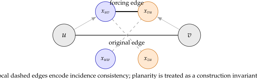
For every processed edge , Furones creates and , assigns weight , solves a Baker-style weighted auxiliary Dominating Set candidate, and decodes selected incidence vertices by first coordinate. In symbols,
The last arrow is deliberately conservative: is only a candidate in the pool.
3.5. Max-Cut Double-Cover Candidate
Furones also derives a candidate from a maximum-cut reduction on the bipartite double cover of the working graph H. The double cover replaces each vertex by two copies and , and each edge by the two crossing edges and (Figure 4). By construction is bipartite, with classes and , so its maximum cut equals . Among all maximum cuts, Furones selects one that minimises the number of copies placed on side 1: it 2-colours each connected component of by breadth-first search and puts the smaller colour class of that component on side 1. Decoding the first coordinates of the minimised side yields the candidate , which is admitted only if it dominates H after pruning (Algorithm 10).
3.5.0.3. Correctness and Running Time
The graph is bipartite by construction—its two classes are and and every edge joins one class to the other—so its maximum cut equals and is realised by any 2-colouring that separates the classes of each connected component. The only freedom is a global flip per component, so placing the smaller colour class of each component on side 1 minimises exactly; this is the standard bipartite min-side maximum cut, computed by one BFS pass. The decoded set carries no structural domination guarantee and enters the portfolio only as a candidate: it is pruned and validated on H before it can be selected (Remark 2), so it cannot compromise feasibility. Building costs time and space (, ); the min-side maximum cut is a single BFS 2-colouring, ; and decoding is . Hence is computed in time.
3.6. Reductions and Their Soundness
We now make the reductions precise—the TSCC cascade and the Baker-style reduced-instance solve—so that the feasibility argument of Section 4 rests on stated lemmas rather than on informal description. Throughout, is the non-isolated working graph; for we write , and SdominatesH iff .
3.6.0.4. The TSCC Cascade
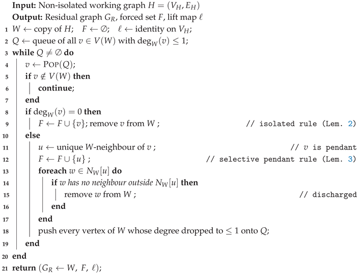
The routine ReduceToTSCCForDS (Algorithm 1) maintains a working graph W, a forced set F of vertices already committed to the solution, and a lift map ℓ. It applies two domination-preserving local rules until neither fires: the isolated rule (Lemma 2), which commits any vertex that has become isolated in W, and the selective pendant rule (Lemma 3), which commits the support u of a pendant v and deletes only the discharged part of , exactly as in Figure 1. The output is a triple in which is the residual graph, F the forced set, and ℓ the map lifting a residual solution back to original labels; the implementation forms the lifted candidate .
| Algorithm 1: ReduceToTSCCForDS — isolated/pendant cascade |
 |
Spanning-Subgraph Monotonicity
The implementation solves the reduced graph directly with the Baker-style routine and admits the result only as a validated candidate. The following monotonicity fact underlies the feasibility argument: a dominating set obtained on any spanning subgraph of (for instance a spanning forest, were one used) still dominates , so solving a sparser surrogate and validating is sound.
Lemma 1
(Spanning-subgraph monotonicity). Let be a spanning subgraph of , that is . If dominates , then D dominates H.
Proof.
Fix . Because D dominates , there exists with , i.e. or . Since , in either case . As w was arbitrary, . □
Corollary 1
(Spanning-subgraph soundness). Every dominating set of a spanning subgraph is a dominating set of . Hence solving a sparser surrogate of can onlyincrease, never invalidate, the size of a residual solution, and the lifted candidate is admitted only after it passes the explicit domination check on H.
Proof.
Apply Lemma 1 with and . The size statement follows because feasibility is preserved while no vertices are removed from the solution; the validation clause is the conservative admission rule of the portfolio. □
Baker’s Technique on the Residual
On a planar residual we use a Baker-style layering: root a breadth-first search, group vertices by BFS layer index modulo , delete one residue class, and solve the remaining bounded-outerplanarity components by dynamic programming [11]. We stress that Dominating Set has boundary effects under layer deletion—a deleted-layer vertex must still be dominated, and domination can cross layer boundaries—so a fully proved planar scheme requires the standard boundary-state dynamic program, which we do not reproduce here. We therefore treat this branch as a validated candidate generator rather than a proved PTAS component: its output enters the pool only as a candidate and is admitted only after the explicit domination check (Corollary 1), and none of the paper’s unconditional guarantees (Theorems 1 and 3) depend on it.
The Salvador Auxiliary Reduction
We record the auxiliary construction of Section 3.4 formally.
Definition 1
(Salvador auxiliary graph). Given G, the auxiliary graph has, for each edge , two incidence vertices and joined by a forcing edge, with placed in the left class and in the right class; the weight of is . The decode map is . Furones solves a Baker-style weighted Dominating Set candidate on , obtains a selected incidence set , and forms the original-graph candidate .
Remark 1
(Salvador soundness is by validation only). No structural soundness is claimed for : it enters the pool as a candidate and is admitted only if, after pruning, it dominates G. This is the deliberately conservative last arrow of the diagram in Section 3.4, and it is why an imperfect auxiliary objective cannot compromise feasibility.
3.7. Main Algorithm
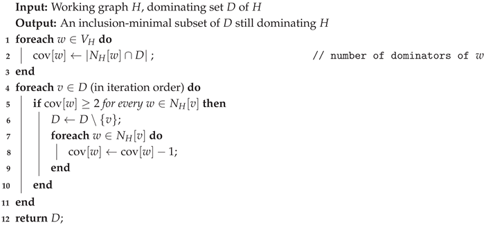
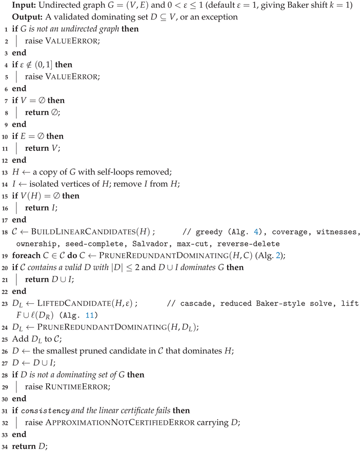
We give the redundancy-removal subroutine and the top-level routine here; the candidate generators—including the dynamic greedy maximum-coverage dominator (Algorithm 4), which certifies Theorem 3—are collected in Section 3.8. Algorithm 2 is the redundancy-removal pass applied to every candidate before the minimum is taken; it underlies Lemma 4.
| Algorithm 2: PruneRedundantDominating — redundancy removal |
 |
| Algorithm 3: Furones: FindDominatingSet |
 |
3.8. Candidate-Generator Pseudocode
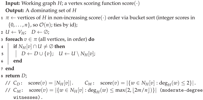
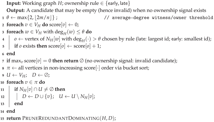
We now give the pseudocode of every candidate generator invoked by BuildLinearCandidates, so that the validity arguments of Section 4.1 can refer to explicit code. The dynamic greedy maximum-coverage generator is Algorithm 4; it re-evaluates each vertex’s coverage gain after every selection (in contrast to the static sweep ) and is the candidate that certifies the guarantee of Theorem 3. The three coverage/witness sweeps share a single routine (Algorithm 5) instantiated with three scoring functions; the remaining generators are Algorithms 6–11.
| Algorithm 4: GreedyMaxCoverage — linear-time dynamic greedy candidate |
 |
| Algorithm 5: CoverageSweep — generates , , |
 |
| Algorithm 6: OrderOwnership — generates |
 |
| Algorithm 7: SeedAndComplete — generates |
 |
| Algorithm 8: ReverseDelete — generates |
 |
| Algorithm 9: SalvadorAuxiliary — generates |
 |
| Algorithm 10: MaxCutDoubleCover — generates |
 |
| Algorithm 11: LiftedCandidate — generates |
 |
4. Correctness of Returned Solutions
The unconditional correctness claim is feasibility. The implementation does not return an unverified candidate.
Lemma 2
(Isolated rule). Let v be isolated in the current working graph and not already dominated by a previously forced vertex. Then every feasible dominating set of the remaining instance contains v.
Proof.
If v has no available neighbour, the only vertex in its closed neighbourhood is v itself. Hence v must be selected. □
Lemma 3
(Pendant rule). Let v be pendant in the current working graph H, and let u be its unique H-neighbour. If v is not already dominated by the forced set, then there is an optimal local choice selecting u rather than v.
Proof.
The closed neighbourhood dominated by v inside the local pendant structure is contained in the domination reach of u for the purpose of covering v and its incident structure. Replacing v by u preserves domination of v and cannot reduce domination within the local closed neighbourhood. The implementation removes only vertices whose remaining responsibilities are discharged, as shown in Figure 1. □
Lemma 4
(Pruning preserves domination). If D dominates G andPruneRedundantDominatingremoves a vertex v only when every vertex in remains dominated by another selected vertex, then the pruned set also dominates G.
Proof.
Deleting v can only change domination counts inside . The removal test checks exactly those vertices and requires an alternate selected dominator for each. Vertices outside are unaffected. Repeating this finite operation preserves domination by induction over the deletion sequence. □
4.1. Validity of the Individual Candidates
Feasibility of the final output rests on each candidate that survives selection being a dominating set. We separate the candidates into those that dominate Hby construction and those that are intentionally selective and therefore admitted only after the explicit per-candidate domination test. Throughout, denotes closed neighbourhoods in the working graph H.
Lemma 5
(Constructive candidates are dominating sets). Each of the following generators returns a set that dominates H by construction: the greedy maximum-coverage candidate , the closed-degree sweep , the low- and medium-degree witness sweeps and , the seed-and-complete candidate , and every reverse-delete candidate .
Proof.
We argue each in turn.
Greedy (Algorithm 4). The routine maintains the set U of still-undominated vertices together with the invariant for every unselected vertex v; because a fresh copy of v is held in bucket whenever its gain changes, the lazy-deletion pop returns a vertex s of maximum current gain (stale or already-selected copies are discarded on pop). The main loop exits only when , and while any satisfies , so the maximum gain is at least 1 and the selected s removes at least one vertex from U. The loop therefore terminates with , i.e. every vertex lies in the closed neighbourhood of a selected vertex. Hence dominates H.
Coverage sweeps (Algorithm 5). Each scans all vertices of H in a fixed order (by closed degree, by low-degree witness score, by medium-degree witness score, respectively) and selects the current vertex whenever it still dominates an undominated vertex. Take any . When the scan reaches u, if u is not yet dominated then is itself undominated, so the selection rule fires and u is dominated. Since the scan visits every vertex, none is left undominated, so each of dominates H; the three differ only in scan order, not in this guarantee.
Seed-and-complete (Algorithm 7). For each seed, the completion phase performs a final pass that adds every still-undominated vertex to the partial set; adding u dominates u because . Each completed seed set therefore dominates H, and returns the smallest such set.
Reverse-delete (Algorithm 8). Each deterministic order starts from the full vertex set , which dominates H trivially, and deletes a vertex only when the resulting set still dominates H. “Dominates H” is thus a loop invariant, so every reverse-delete candidate dominates H. □
Lemma 6
(The lifted candidate is a dominating set). If the reduced solve returns a dominating set of the reduced graph , then the lifted candidate produced by Algorithm 11 dominates H.
Proof.
Since dominates (the Baker-style routine repairs separator domination; Corollary 1 additionally covers any sparser surrogate of ), dominates the vertices that survive the cascade. The forced set F accumulated by the cascade dominates the removed vertices: each vertex deleted by the isolated rule is placed in F (Lemma 2), and each vertex discharged by the pendant rule lies in for the forced support (Lemma 3), where u is removed only because it has no responsibility outside . Hence every vertex of H is dominated by F or by , so dominates H. □
Remark 2
(Selective and auxiliary candidates are validation-filtered). The order-ownership candidates , the Salvador auxiliary candidate , and the max-cut double-cover candidate are intentionally selective and arenotguaranteed to dominate H by construction: order ownership (Algorithm 6) returns the empty set whenever no vertex receives a positive ownership score, which fails to dominate a non-empty graph (consistent with being valid on of the CAR-002 instances of Table 3); the Salvador candidate (Algorithm 9) carries no structural soundness claim (Remark 1); and the max-cut candidate (Algorithm 10) decodes a min-side maximum cut of the double cover, which need not dominate H. The portfolio therefore tests every candidate for domination of H and discards those that fail; the minimum in Algorithm 3 is taken only over candidates that dominate H.
Corollary 2
(The validated candidate pool is non-empty). For every working graph H at least one candidate—for instance by Lemma 5—dominates H. Hence the set of valid candidates over which Algorithm 3 minimises is non-empty and consists only of dominating sets of H.
Theorem 1
(Feasibility of Furones outputs). Whenever Algorithm 3 returns normally, its output D is a dominating set of the original input graph G.
Proof.
The preprocessing handles isolated vertices separately and ignores self-loops, which do not affect domination in simple undirected graphs. Lemmas 2 and 3 justify the local forced choices made during the cascade. By Lemma 5 the constructive candidates () dominate H, and by Lemma 6 so does the lifted candidate ; the selective and auxiliary candidates () are admitted only after passing the explicit domination test (Remark 2). Corollary 2 therefore guarantees that the pool over which the algorithm minimises is non-empty and contains only dominating sets of H. Lemma 4 shows that the pruning pass of Algorithm 2 cannot destroy domination for any candidate that was already feasible. Finally, before returning, the implementation calls a direct domination check on the original graph after reinserting isolated vertices. If that check fails, it raises an exception instead of returning. Therefore every normal return is a dominating set of G. □
5. Complexity Analysis
We give a per-subroutine worst-case analysis rather than a global assertion that “everything is a graph scan.” Throughout, , , and is the maximum degree; the implementation uses adjacency lists, so a single pass over all closed neighbourhoods costs . We first bound the two subroutines on which the approximation guarantee depends, then account for the whole pipeline.
Lemma 7
(Greedy and pruning run in linear time). With adjacency lists and a bucket priority queue keyed by current coverage gain, Algorithm 4 runs in time and space, and Algorithm 2 runs in time and space.
Proof.
Greedy. Maintain buckets holding the vertices of current gain and a pointer to the largest non-empty bucket. Initialisation costs for the buckets and for the initial gains . Each selection pops the top bucket in . The only operations that change gains are the decrements , each of which moves z down one bucket in . A decrement occurs once for every incidence with at the moment w is first covered; since every vertex w is covered exactly once, the total number of decrements is . Because gains never increase, the top pointer is non-increasing and moves downward at most times in total. Hence the running time is .
Pruning. Computing the dominator counts costs . Each is examined once; its removability test and the subsequent count updates touch only , costing . Summing over D gives . □
Theorem 2
(Linear runtime with a large constant). Let and . For fixed Baker parameter ε (default , giving ), a fixed seed limit s, a fixed bucket count b, and a fixed number r of deterministic reverse-delete orders, the implemented Furones v0.3.8 pipeline runs in time and uses space. The hidden constant is large; on the general planar Baker branch it grows as , which equals 3 for the default .
Proof.
We bound each stage; let and denote the size of the reduced instance.
| Stage | Worst-case time |
| Self-loop removal, isolate detection,closed-neighbourhood marking | |
| TSCC cascade, queue-based (Algorithm 1) | |
| Reduced Baker-style solve (BakerPTAS, , ) | |
| Lift | |
| Greedy and static coverage (Lemma 7) | |
| Witness scores and ownership | |
| Seed-and-complete (s seeds, passes each) | |
| Salvador auxiliary : build () + planar Baker solve () | |
| Max-cut double cover (Alg. 10):build ( nodes, edges) + BFS min-side cut | |
| Reverse-delete (r deterministic orders) | |
| Prune every candidate (Algorithm 2,Lemma 7) | per candidate |
| Final domination validation on G |
The cascade is linear because each vertex enters the queue times and every deletion charges to an incident edge, so the total edge work is . There are candidate families and each is pruned once; summing the table and absorbing the fixed parameters , s, b, r into a single constant gives total bound . Every stage stores only words (the working graph, the auxiliary graph of size , bucket arrays, and per-vertex counters), so the space bound is .
The constant c is intentionally not small. Furones pays for several independent candidates because different candidates win on different graph families. With the default (Baker shift ) the reduced-solve factor is the constant 3, so it does not affect the asymptotic order. The asymptotic order in is unaffected by any of these choices once are fixed. □
6. Approximation Ratio Analysis
We separate two very different statements. The first is an unconditional approximation theorem that we prove here, parameterised by the maximum degree . The second is the near-threshold ratio , which still crosses the known hardness frontier and is therefore recorded as a named hypothesis with its complexity-theoretic consequence and partial evidence.
6.1. An Unconditional Degree-Parameterised Guarantee
Theorem 3
(Degree-parameterised approximation). For every finite undirected graph G with maximum degree Δ, Algorithm 3 returns a dominating set D with
where is the k-th harmonic number. In particular, for the class of graphs with the ratio is : a sub-logarithmic-in-n approximation guarantee.
Proof.
The preprocessing splits G into its isolated vertices I and the non-isolated working graph H. Every isolated vertex is forced into every dominating set, hence into both the returned set and any optimum, so and the returned set has the form . It therefore suffices to prove , since adding the common term (valid as ) to both sides preserves the inequality and yields .
Cast Dominating Set on H as a Set Cover instance with universe and one set for each . A subfamily covers if and only if dominates H; hence the optimum of this Set Cover instance equals , and every set has size . Algorithm 4 is precisely the greedy Set Cover heuristic on this instance: at each step it selects the vertex whose closed neighbourhood covers the largest number of still-uncovered elements, updating the residual coverage afterwards. By the classical analysis of Johnson, Lovász, and Chvátal, greedy returns a cover of size at most , where s is the maximum set size [1,2,3]. Here and , so the greedy candidate satisfies .
Finally, the portfolio returns the smallest pruned valid candidate, and is one such candidate (it dominates H by construction). Pruning only removes vertices (Algorithm 2), so . Using the standard estimate gives . When we have , the claimed sub-logarithmic-in-n guarantee. □
Corollary 3
(Constant factor on bounded-degree graphs). On any family of graphs of bounded maximum degree , Furones is a polynomial-time constant-factor approximation for Minimum Dominating Set, with ratio at most .
Proof.
Immediate from Theorem 3: with the factor is a constant. This does not contradict the hardness frontier, because Dominating Set restricted to bounded-degree graphs is constant-factor approximable. □
Remark 3
(Why this is the achievable frontier in n). The guarantee is essentially the best obtainable as a function of n alone. When we have , matching the greedy guarantee for general Set Cover, and the tightness of that analysis [4] shows the factor cannot be improved by a sharper analysis of greedy by itself. Lowering then-dependencebelow uniformly over all graphs is exactly what the hardness results forbid: by Dinur–Steurer, any polynomial-time approximation for general Dominating Set with ratio in n implies [5,6,7]. Theorem 3 thus sits exactly at the achievable frontier.
6.2. A Near-Threshold Ratio Hypothesis
The degree-parameterised guarantee of Theorem 3 is logarithmic only in the worst case . We now record, as an explicit conditional hypothesis, the weaker claim that Furones meets a fixed sub-threshold ratio on all graphs—weaker than a constant ratio, but still strong enough to cross the inapproximability frontier—and we give partial evidence for it.
Hypothesis 1
(Furones near-threshold ratio hypothesis). Let and put . For every finite undirected graph G, Algorithm 3 returns a dominating set D satisfying
Remark 4
(On the word “sub-logarithmic”). The factor has the same growth order as —it is , not —so it is not sub-logarithmic in the asymptotic sense. What matters for hardness is theleading constant: with , which lies strictly below the optimal inapproximability threshold. It is in this precise “sub-threshold” sense that the hypothesis is a strong claim, and it is exactly this property that forces the implication below.
Theorem 4
(Complexity-theoretic consequence). If Hypothesis 1 is proved for Furones on arbitrary finite graphs, then .
Proof.
For all we have , hence , and the hypothesis asserts a polynomial-time (Theorem 2) approximation of Minimum Dominating Set within the ratio with . By the optimal hardness of Dinur–Steurer, building on Feige and on Raz–Safra, no polynomial-time algorithm approximates general Dominating Set within for any fixed unless [5,6,7]. Applying this with contradicts the hypothesis unless . □
We now give evidence that, despite this consequence, the hypothesis is far less speculative than a blanket constant-ratio claim: it is already a Theorem for every graph except the high-degree ones.
Proposition 1
(The hypothesis is unconditional below degree ). Let . For every finite graph G on n vertices with maximum degree , the bound of Theorem 3 already yields
so Hypothesis 1 holds unconditionally on G. Consequently the only graphs for which the hypothesis is open are those with ; for this means , i.e. above a constant multiple of (not necessarily ).
Proof.
By Theorem 3, . If , then . Otherwise , i.e. , so
In either case , which gives the claim. The two thresholds coincide at , so for the active bound is . □
6.2.0.8. High-Degree Graphs on Which the Hypothesis Is Already a Theorem
Proposition 1 leaves open only the regime . We now show that even there the hypothesis is provable on broad structural families, and we pin down precisely what an instance must look like to escape these proofs. The governing parameter is how far exceeds its trivial packing lower bound .
Definition 2
(Domination tightness). For a graph G on n vertices with maximum degree Δ, thedomination tightnessis
Here exactly when G admits anefficient dominating set(a perfect code: the closed neighbourhoods of an optimum partition V), and increases as moves above the packing bound.
Theorem 5
(High-degree provable regime). Let G have n vertices, minimum degree δ, maximum degree Δ, and domination number . The portfolio output D satisfies
Consequently the near-threshold hypothesis holds whenever
Proof.
We bound the greedy candidate directly by an averaging argument. While a set U of vertices is still undominated, every has , so
and hence some vertex covers at least of U. Each greedy selection therefore multiplies the undominated count by at most , so after at most selections the undominated set has size at most ; adding those remaining vertices yields
the algorithmic minimum-degree domination bound (the greedy form of the Arnautov–Payan–Alon bound [12]). The portfolio returns the smallest pruned valid candidate, so . Writing from Definition 2 and dividing gives the stated ratio; the sufficient condition is its rearrangement. □
Corollary 4
(Regular and near-regular dense graphs). If G is d-regular then , so the hypothesis holds whenever
If G is only α-near-regular, , the hypothesis holds whenever . For and the regular threshold lies in , so the hypothesis can fail on a regular graph only if is within a factor below 2 of the bare packing bound .
Proof.
Set in Theorem 5; the near-regular case substitutes . For we have , and for the ratio ranges over . □
Corollary 5
(Very dense and dominating-vertex graphs). The hypothesis holds for every graph with a dominating vertex, where and the greedy candidate returns ; and for every near-complete graph with , where the trivial dominating set for a maximum-degree vertex v has size at most .
Remark 5
(Where the unresolved regime is concentrated). Combining Proposition 1 with Theorem 5 and its corollaries, the regime not settled by the proofs above is narrow and structured. Theorem 5 controls a high-degree graph once , which holds for regular and near-regular graphs whose tightness exceeds the small threshold of Corollary 4, for very dense graphs, and for graphs with a dominating vertex. This sufficient condition can fail in two ways: when the domination tightness is within a sub-logarithmic factor of 1 (a domination number close to the packing bound ), or when the graph is strongly irregular (a large gap between maximum and minimum degree, which inflates the factor ). We therefore state the residual regime as a narrowing principle rather than an exhaustive classification:the unresolved instances are concentrated around high-degree graphs whose domination number nearly attains the closed-neighbourhood packing lower bound —the (near-)perfect-coderegime of efficient or almost-efficient dominators on dense, highly symmetric structures such as Hamming graphs and certain circulants. On these the hypothesis reduces to whether the greedy and seed candidates recover the (near-)perfect code, which the reproducible high-degree experiment of Section 7.2 (CAR-003) probes directly: across 1000 dense instances with , including perfect-code cases, the returned set is optimal on every instance (hence within throughout).
Remark 6
(Evidence for the remaining high-degree regime). Proposition 1 reduces the hypothesis to graphs of maximum degree (above a constant multiple of ), and three independent strands of evidence point the same way there, though none is a proof. First, the high-degree regime is exactly thedenseregime, where covering problems are known to admit far better than logarithmic approximation: dense instances of Set Cover and related covering problems have constant- and sub-threshold approximations [13]. Second, very dense graphs have a small optimum: taking a maximum-degree vertex v and adding every vertex outside yields a dominating set, so , which is tiny when Δ is close to n; a small is precisely where the constant floor 4 in is most forgiving and where the greedy candidate and the seed-completion candidate empirically return optima. Third, the exact CAR benchmark of Section 7 includes a dense Erdos–Rényi family and reports an observed ratio of on every instance, far inside . Fourth, Theorem 5 and Corollaries 4–5 convert most of the high-degree regime from claim into proof: regular and near-regular dense graphs (whose tightness τ exceeds the small threshold of Corollary 4), very dense graphs, and graphs with a dominating vertex all satisfy the hypothesis unconditionally. By Remark 5 the unresolved instances are concentrated around the (near-)perfect-code graphs whose domination number nearly meets the packing bound , together with strongly irregular high-degree graphs not covered by the min-degree bound. We stress that, beyond the parts now proved, this residual regime remains a conditional claim, not a proof: by Theorem 4 a full proof of it would settle .
Remark 7
(What is and is not proved here). Theorem 4 is a consequence statement, not a proof that . The paper proves three unconditional results: feasibility (Theorem 1); the degree-parameterised approximation guarantee (Theorem 3), a constant factor on bounded-degree graphs (Corollary 3); and the near-threshold ratio for all graphs of maximum degree (Proposition 1). Only the high-degree case of Hypothesis 1 is open; by Remark 4 and Theorem 4, proving it would require new approximation theory strong enough to settle the complexity-theoretic barrier.
7. Experimental Study: Exact CAR Benchmarks
The core CAR benchmark contains 1000 deterministic small graphs over seven families: sparse, medium, and dense Erdős–Rényi graphs, random bipartite graphs, random trees, perturbed paths/cycles, and small structured graphs. Every graph has at most 14 vertices, so the script first computes the exact domination number by exhaustive search and then compares Furones v0.3.8 with that optimum. Table 2 summarises car/family_summary.csv. On this finite exact benchmark, Furones returns a valid optimum on all 1000 instances, so the observed benchmark constant is . Because every tested instance is small ( across all three studies), throughout, so the binding value of is the constant floor 4. These experiments should therefore be read as exact evidence against factor-4 violations on small instances, not as evidence for the asymptotic part of the near-threshold hypothesis.
7.1. Where Each Strategy Wins
The central empirical lesson is that the portfolio is doing real work. The greedy maximum-coverage candidate that certifies Theorem 3 is part of the portfolio; the ablation below reports the strategies instrumented in the released v0.3.8 CAR artifact, where the closed-degree sweep is the corresponding coverage entry. Table 3 summarises car/strategy_ablation_summary.csv. A strategy is counted as optimal when its own pruned candidate has size , and it is counted as min-attaining when it ties for the smallest valid candidate among the measured strategy pool. Ties count for every tied strategy.

Table 3.
Per-strategy ablation on the 1000-instance exact CAR benchmark (Furones v0.3.8). “Optimal / min” is both the percentage of instances where the strategy matched and the percentage where it attained the minimum valid candidate size among measured strategies; in this benchmark those two percentages coincide because at least one measured strategy is optimal on every instance.
Table 3.
Per-strategy ablation on the 1000-instance exact CAR benchmark (Furones v0.3.8). “Optimal / min” is both the percentage of instances where the strategy matched and the percentage where it attained the minimum valid candidate size among measured strategies; in this benchmark those two percentages coincide because at least one measured strategy is optimal on every instance.
| Strategy | Valid | Optimal / min | Mean size | Mean ratio | Max ratio |
|---|---|---|---|---|---|
| Seed-and-complete | 100.0% | 99.8% | 3.799 | 1.000 | 1.250 |
| Greedy max-coverage () | 100.0% | 92.7% | 3.870 | 1.023 | 1.500 |
| Closed-degree coverage | 100.0% | 89.0% | 3.923 | 1.048 | 2.500 |
| Reverse delete, low-degree order | 100.0% | 88.7% | 3.926 | 1.049 | 2.500 |
| Medium-degree witnesses | 100.0% | 88.3% | 3.932 | 1.054 | 2.500 |
| TSCC/Baker/lift | 100.0% | 87.8% | 3.925 | 1.052 | 2.000 |
| Salvador auxiliary | 100.0% | 84.9% | 3.991 | 1.107 | 5.000 |
| Low-degree witnesses | 100.0% | 84.8% | 3.985 | 1.080 | 3.000 |
| Order ownership, late | 79.2% | 65.8% | 3.643 | 1.060 | 2.000 |
| Order ownership, early | 79.2% | 64.5% | 3.659 | 1.065 | 2.000 |
| Reverse delete, reverse input | 100.0% | 61.2% | 4.336 | 1.176 | 3.500 |
| Max-cut double cover () | 100.0% | 58.4% | 4.345 | 1.217 | 5.000 |
| Reverse delete, input order | 100.0% | 57.9% | 4.417 | 1.241 | 5.000 |
| Reverse delete, high-degree order | 100.0% | 27.9% | 5.003 | 1.428 | 5.000 |
On this exact small-graph benchmark, seed-and-complete is the strongest single candidate, matching the optimum on of instances, and the greedy maximum-coverage candidate that certifies Theorem 3 matches it on (mean ratio ). Closed-degree coverage, low-degree reverse delete, medium-degree witnesses, TSCC/Baker/lift, Salvador auxiliary, and low-degree witnesses each match the optimum on at least of instances. Order-ownership candidates are less frequently valid because they are intentionally selective, but when valid their ratios remain small. The new max-cut double-cover candidate is always valid but weaker on its own (optimal on , mean ratio ); like the reverse-delete orders, it mainly widens the pool from which the minimum-selection step draws. No single strategy is globally optimal, but that step combines them: the final portfolio returns an exact optimum on all 1000 instances.
7.2. Small Instances Above the Threshold (CAR-003)
Proposition 1 proves the near-threshold hypothesis for all graphs of maximum degree , leaving the high-degree regime to Theorem 5 and its corollaries. To probe that regime directly we ran the reproducible experiment car/run_high_degree_experiment.py (base seed 12345, 1000 instances), which generates small instances that all clear the formal threshold across seven (typically dense) families (complete, cocktail-party, dense circulant, random-regular, dense Erdős–Rényi, perturbed hypercube, perturbed Paley), computes the exact domination number by increasing-size exhaustive search, and compares it with the set returned by the installed Furones v0.3.8 solver—the full portfolio, invoked via from furones.algorithm import find_dominating_set. The pool deliberately includes perfect-code stress cases—complete graphs, dense circulants, hypercubes, and Paley graphs—many of which have domination tightness , exactly the case identified as potentially hardest in Remark 5. Because n is small, some instances clear with only modest absolute degree (for example or 3); we therefore read CAR-003 as exact evidence on small instances above the threshold, not as asymptotic dense-graph evidence. Table 4 summarises car/CAR-003-high-degree.json.
The outcome supports Hypothesis 1 in exactly the regime the theory could not fully close: all 1000 high-degree instances return within and are solved optimally, so the overall mean and maximum ratio are both with zero violations. In particular every perfect-code instance—the case flagged as potentially hardest in Remark 5, spanning complete graphs, efficient circulants, hypercubes, and Paley graphs—is solved optimally, so the full portfolio recovers the (near-)perfect code wherever one occurs in the pool. As with Section 7, this is exact finite evidence over a bounded instance pool, not a proof of the residual case.
7.3. Adversarial Worst-Case Stress Test (CAR-004)
CAR-003 samples natural dense families; CAR-004 instead actively hunts for the worst instances for the hypothesis. The reproducible experiment car/run_adversarial_experiment.py (base seed 1000) generates graphs from seven adversarial families: greedy traps (private blocks behind decoy-inflated centres), the tight set-cover-to-domination gadget with geometric decoys, perturbed perfect-code graphs, near-efficient circulants, cocktail-party and complete-multipartite graphs (whose optimum is 2, stressing the constant floor), dense random-regular graphs, and dense Erdos–Rényi graphs. Every family is engineered so that the optimum stays small, so the exact is computed quickly by increasing-size exhaustive search from the packing lower bound; this keeps the full -instance comparison against the optimum feasible. Because all feasible instance sizes satisfy , the binding bound throughout is the constant floor : CAR-004 directly asks whether any adversary can drive Furones above . Table 5 summarises car/CAR-004-adversarial.json.
No adversarial instance produced a violation: the largest ratio anywhere in the -instance sweep was , comfortably under the binding bound , and the mean ratio was . Even the constructions specifically designed to defeat greedy selection (greedy traps and the geometric set-cover gadget) were solved optimally on every instance, because the portfolio’s validation, pruning, and reverse-delete candidates recover the small optimum that the decoys try to hide. Together with CAR-003 this gives strong finite evidence for Hypothesis 1 across both the natural dense regime and an explicit adversarial search, while remaining, by Theorem 4, short of a proof.
Reproducibility of the CAR Artifacts
All four CAR studies were run against the public Furones v0.3.8 release installed with pip install furones and invoked as from furones.algorithm import find_dominating_set, so the reported numbers reflect the released solver rather than a re-implementation. The rerun scripts and machine-readable outputs are provided in the repository’s car/ folder.
8. Discussion
8.1. Empirical vs. Theoretical Gap
The exact CAR benchmarks are encouraging but still finite. The 1000-instance core benchmark verifies that Furones v0.3.8 returns exact optima on a broad small-graph sample with exhaustive optimum certificates, without using an exact solver inside Furones itself. The high-degree probe (CAR-003) extends this to 1000 dense instances with —including perfect-code cases—on which the solver is optimal throughout, and the adversarial stress test (CAR-004) records no violation of across worst-case instances. The shared limitation is scale: the graphs are deliberately small enough for exact search, so the benchmarks measure finite evidence rather than asymptotic approximation behaviour.
The theoretical picture now has three layers. Feasibility is unconditional (Theorem 1). The degree-parameterised ratio is also unconditional (Theorem 3): it is sub-logarithmic in n for graphs of sub-polynomial maximum degree and a constant factor on bounded-degree graphs. Only the near-threshold -ratio statement (Hypothesis 1) remains open, and even there Proposition 1 settles it for all graphs of maximum degree ; Theorem 4 shows a full proof would imply , so the paper treats the remaining high-degree case as the central open mathematical target rather than as a settled guarantee.
8.2. Hardness Barriers
For Minimum Dominating Set, any fixed constant approximation factor is already below the asymptotic logarithmic hardness threshold on sufficiently large graphs. This is why the manuscript treats any universal constant-ratio claim with special care: such a theorem would not merely be a better analysis of a known approximation algorithm; it would collapse the standard hardness landscape for Dominating Set.
8.3. Comparison to Standard Methods
The classical greedy Set Cover style approach gives an approximation for Dominating Set [1,3,14]. Furones contains exactly this greedy as its candidate , so it inherits the same worst-case guarantee (Theorem 3) while the minimum-selection step can only improve on it; the static sweep is a cheaper surrogate that forgoes the guarantee. Exact algorithms and integer programming can certify optima on small or structured graphs, but they do not give the same large-input linear profile. Furones occupies a distinct design point: a validated linear-time portfolio with a large constant, the provable degree-parameterised ratio, exact behaviour across the CAR benchmarks, and an explicit near-threshold ratio hypothesis whose proof would have major complexity consequences.
9. Conclusion
This paper has presented Furones v0.3.8 for Minimum Dominating Set. Furones is a linear-time, large-constant candidate-comparison algorithm combining TSCC-style reduction, Baker-style planar solving, original-graph coverage and witness sweeps, order ownership, seed completion, a Salvador-style auxiliary path, reverse-delete scans, pruning, and direct validation. We proved two unconditional guarantees: feasibility (every normal return is a dominating set of the original graph) and a degree-parameterised approximation ratio , obtained because the portfolio contains the dynamic greedy maximum-coverage dominator. This ratio is sub-logarithmic in n for every graph of sub-polynomial maximum degree and a constant factor on bounded-degree graphs, and it sits exactly at the -in-n hardness frontier.
The stronger near-threshold ratio claim is stated as Hypothesis 1: Furones meets ratio on every graph. Proposition 1 already proves it for all graphs of maximum degree ; if a proof is supplied for the remaining high-degree graphs, then Furones approximates general Minimum Dominating Set within in polynomial time, and Theorem 4 shows that this would imply . The exact CAR benchmarks support the current engineering claim that the candidate portfolio is strong on small certified instances—all 1000 core-benchmark ratios equal , and the high-degree and adversarial studies record no violation of —but they do not by themselves prove the near-threshold ratio hypothesis.
Availability. The Furones algorithm is distributed via PyPI:
- Package:https://pypi.org/project/furones
- Repository:https://github.com/frankvegadelgado/furones
- Installation:pip install furones
- Usage:from furones.algorithm import find_dominating_set
Code and data: https://github.com/frankvegadelgado/furones (stable release tag v0.3.8, corresponding to the manuscript). The CAR-style measurement artifacts and human-readable Integrity Report are provided in the repository’s car/ folder.
The repository’s car/ folder contains a CAR manifest, CAR.furones-v0.3.8.json, plus detailed JSON/CSV measurement artifacts and the human-readable INTEGRITY_REPORT.md. The artifacts document four checks: (i) the observed finite-benchmark constant obtained from 1000 exact small-graph instances (CAR-001); (ii) a per-strategy ablation measuring candidate sizes, optimum-attainment percentages, and min-attainment percentages (CAR-002); (iii) the high-degree dense-regime experiment probing against exact domination numbers (CAR-003); and (iv) the -instance adversarial worst-case stress test (CAR-004). Every study is reproduced by the scripts in car/, run after pip install furones (v0.3.8) and invoked via from furones.algorithm import find_dominating_set.
- Code and data are identified with version pins: Furones v0.3.8 and the repository in https://github.com/frankvegadelgado/furones.
- Prerequisite for every CAR experiment: install the public release with pip install furones (v0.3.8); all rerun scripts then import from furones.algorithm import find_dominating_set, so the reported numbers reflect the installed solver.
- Four exact-optimum CAR studies, candidate outputs, and aggregate percentages are in the repository’s car/ folder; every instance is compared against a domination number computed by exhaustive search.
- The finite-benchmark ratio check is recorded in car/CAR-001-ratio-constant.json (1000 instances), rerun via car/run_integrity_measurements.py.
- The per-strategy ablation, including the dynamic greedy maximum-coverage candidate, is recorded in car/CAR-002-strategy-ablation.json (same rerun script).
- The high-degree / dense-regime experiment (, 1000 instances including perfect-code cases) is recorded in car/CAR-003-high-degree.json, rerun via car/run_high_degree_experiment.py.
- The -instance adversarial worst-case stress test is recorded in car/CAR-004-adversarial.json, rerun via car/run_adversarial_experiment.py; it reports zero violations of .
- A human-readable Integrity Report covering all four studies is supplied as car/INTEGRITY_REPORT.md.
- All ratio observations are finite-benchmark evidence with exact optima; the unconditional results in the paper are feasibility and the degree-parameterised guarantee. The near-threshold ratio hypothesis is proved for and for regular, near-regular, and very dense graphs, leaving the residual regime concentrated around the (near-)perfect-code case; none of this is treated as a universal approximation proof.
No human subjects; wider-impact discussion included through the approximation-hardness and versus interpretation.
Funding
This research did not receive any specific grant from funding agencies in the public, commercial, or not-for-profit sectors.
Acknowledgments
The author would like to thank Iris, Marilin, Sonia, Yoselin, Arelis, and Royce for their support.
Conflicts of Interest
The author declares no competing interests.
Use of Artificial Intelligence
During the preparation of this work the author used AI assistants (ChatGPT and Claude) to improve the readability of the manuscript and to design and run the reproducible exact CAR experiments summarized in Table 2, Table 3, Table 4, and Table 5. After using these tools, the author reviewed and edited the content as needed and takes full responsibility for the content of the publication.
References
- Johnson, D.S. Approximation algorithms for combinatorial problems. J. Comput. Syst. Sci. 1974, 9, 256–278. [Google Scholar] [CrossRef]
- Lovász, L. On the ratio of optimal integral and fractional covers. Discret. Math. 1975, 13, 383–390. [Google Scholar] [CrossRef]
- Chvátal, V. A greedy heuristic for the set-covering problem. Math. Oper. Res. 1979, 4, 233–235. [Google Scholar] [CrossRef]
- Slavík, P. A tight analysis of the greedy algorithm for set cover. J. Algorithms 1997, 25, 237–254. [Google Scholar] [CrossRef]
- Feige, U. A threshold of lnn for approximating set cover. J. ACM 1998, 45, 634–652. [Google Scholar] [CrossRef]
- Raz, R.; Safra, S. The distance of the minimum dominating set problem from (lnn)-approximation. In Proceedings of the Proceedings 43rd Annual IEEE Symposium on Foundations of Computer Science, Washington, DC, USA, 2002; pp. 311–320. [Google Scholar]
- Dinur, I.; Steurer, D. Analytical Approach to Parallel Repetition. In Proceedings of the Proceedings of the 46th Annual ACM Symposium on Theory of Computing, New York, USA, 2014; pp. 624–633. [Google Scholar] [CrossRef]
- Vega, F. Furones: Approximate Dominating Set Solver. 2026, Version 0.3.8. Available online: https://pypi.org/project/furones (accessed on 3 July 2026).
- Hagberg, A.A.; Schult, D.A.; Swart, P.J. Exploring network structure, dynamics, and function using NetworkX. In Proceedings of the Proceedings of the 7th Python in Science Conference, 2008; pp. 11–15. [Google Scholar] [CrossRef]
- Virtanen, P.; Gommers, R.; Oliphant, T.E.; Haberland, M.; Reddy, T.; Cournapeau, D.; Burovski, E.; Peterson, P.; Weckesser, W.; Bright, J.; et al. SciPy 1.0: fundamental algorithms for scientific computing in Python. Nat. Methods 2020, 17, 261–272. [Google Scholar] [CrossRef] [PubMed]
- Baker, B.S. Approximation algorithms for NP-complete problems on planar graphs. J. ACM 1994, 41, 153–180. [Google Scholar] [CrossRef]
- Alon, N.; Spencer, J.H. The Probabilistic Method, 4th ed.; John Wiley & Sons: Hoboken, NJ, 2016. [Google Scholar]
- Karpinski, M.; Zelikovsky, A. Approximating Dense Cases of Covering Problems. In Proceedings of the DIMACS Series in Discrete Mathematics and Theoretical Computer Science, Providence, Rhode Island, 1996; Vol. 26, pp. 147–164. [Google Scholar]
- Vazirani, V.V. Approximation Algorithms; Springer Science & Business Media, 2001. [Google Scholar]
Figure 2.
Code-faithful pipeline of Furones v0.3.8. The lower path computes the dynamic greedy maximum-coverage candidate together with the other general linear candidates (coverage/witness sweeps and reverse-delete) on the original working graph; the upper path performs the cascade reduction, Baker-style solving, and lifting. All candidates meet at the prune-and-validate stage.
Figure 2.
Code-faithful pipeline of Furones v0.3.8. The lower path computes the dynamic greedy maximum-coverage candidate together with the other general linear candidates (coverage/witness sweeps and reverse-delete) on the original working graph; the upper path performs the cascade reduction, Baker-style solving, and lifting. All candidates meet at the prune-and-validate stage.
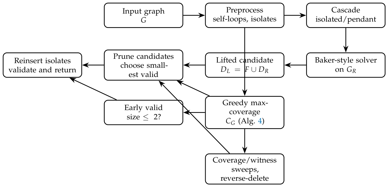
Figure 4.
Bipartite double-cover gadget for the max-cut candidate . Each original edge becomes the crossing edges and , so is bipartite by the second coordinate and every edge is cut. Furones takes a maximum cut minimising one side and decodes the first coordinates of that side as an original-graph candidate.
Figure 4.
Bipartite double-cover gadget for the max-cut candidate . Each original edge becomes the crossing edges and , so is bipartite by the second coordinate and every edge is cut. Furones takes a maximum cut minimising one side and decodes the first coordinates of that side as an original-graph candidate.
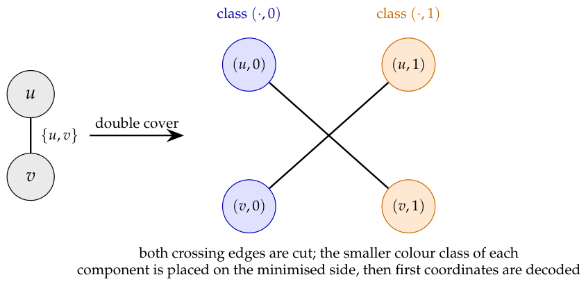
Table 1.
Code metadata for the Furones package.
| Nr. | Code metadata description | Metadata |
|---|---|---|
| C1 | Current code version | v0.3.8 |
| C2 | Permanent link to code/repositoryused for this code version | https://github.com/frankvegadelgado/furones |
| C3 | Permanent link to reproducible capsule | https://pypi.org/project/furones/ |
| C4 | Legal Code License | MIT License |
| C5 | Code versioning system used | git |
| C6 | Software code languages, tools, and services used | Python |
| C7 | Compilation requirements, operatingenvironments, and dependencies | Python ≥ 3.12, NetworkX ≥ 3.4.2 [9], NumPy ≥ 2.2.1, SciPy ≥ 1.15.0 [10] |
| C8 | Main entry points | asia, batch_asia, test_asia; core routine furones.algorithm.find_dominating_set |
Table 2.
Exact CAR benchmark for Furones v0.3.8. Each row uses exhaustive search to compute the exact domination number before comparing the returned set size with .
Table 2.
Exact CAR benchmark for Furones v0.3.8. Each row uses exhaustive search to compute the exact domination number before comparing the returned set size with .
| Family | Instances | n range | range | Optimal outputs | Mean ratio | Max ratio |
|---|---|---|---|---|---|---|
| Erdős–Rényi sparse | 200 | 6–14 | 2–10 | 100.0% | 1.000 | 1.000 |
| Erdős–Rényi medium | 200 | 6–14 | 2–5 | 100.0% | 1.000 | 1.000 |
| Erdős–Rényi dense | 150 | 6–14 | 1–4 | 100.0% | 1.000 | 1.000 |
| Random bipartite | 150 | 6–14 | 2–9 | 100.0% | 1.000 | 1.000 |
| Random trees | 100 | 6–14 | 2–6 | 100.0% | 1.000 | 1.000 |
| Perturbed paths/cycles | 100 | 6–14 | 2–5 | 100.0% | 1.000 | 1.000 |
| Small structured graphs | 100 | 6–14 | 1–4 | 100.0% | 1.000 | 1.000 |
| Overall exact CAR benchmark | 1000 | 6–14 | 1–10 | 100.0% | 1.000 | 1.000 |
Table 4.
CAR-003 high-degree experiment: 1000 dense instances over seven families, all with , solved by the installed Furones v0.3.8 solver and compared against the exact domination number. The returned set lies within on every instance and is optimal on all 1000 (overall mean and maximum ratio ), including every perfect-code instance.
Table 4.
CAR-003 high-degree experiment: 1000 dense instances over seven families, all with , solved by the installed Furones v0.3.8 solver and compared against the exact domination number. The returned set lies within on every instance and is optimal on all 1000 (overall mean and maximum ratio ), including every perfect-code instance.
| Family | Inst. | n | Mean ratio | Max ratio | |||
|---|---|---|---|---|---|---|---|
| Complete | 143 | 6–16 | 5–15 | 1.00 | 1.000 | 1.000 | 100% |
| Cocktail party | 143 | 6–16 | 4–14 | 1.67–1.88 | 1.000 | 1.000 | 100% |
| Dense circulant | 143 | 8–16 | 4–15 | 1.00–1.88 | 1.000 | 1.000 | 100% |
| Random regular | 143 | 8–16 | 2–8 | 1.00–1.69 | 1.000 | 1.000 | 100% |
| Dense Erdos–Rényi | 143 | 8–16 | 4–15 | 1.00–2.44 | 1.000 | 1.000 | 100% |
| Hypercube (perturbed) | 143 | 8–16 | 3–6 | 1.00–1.75 | 1.000 | 1.000 | 100% |
| Paley (perturbed) | 142 | 5–13 | 2–7 | 1.00–1.85 | 1.000 | 1.000 | 100% |
| Overall | 1000 | 5–16 | 2–15 | 1.00–2.44 | 1.000 | 1.000 | 100% |
Table 5.
CAR-004 adversarial stress test: instances drawn from worst-case families and compared against the exact optimum using the installed Furones v0.3.8 solver. Furones returns a valid dominating set on every instance, stays within on of them with zero violations, is optimal on , and attains overall mean ratio . The single worst instance is a dense random-regular graph (, , returned size 4, ratio ), still far below the floor .
Table 5.
CAR-004 adversarial stress test: instances drawn from worst-case families and compared against the exact optimum using the installed Furones v0.3.8 solver. Furones returns a valid dominating set on every instance, stays within on of them with zero violations, is optimal on , and attains overall mean ratio . The single worst instance is a dense random-regular graph (, , returned size 4, ratio ), still far below the floor .
| Adversarial family | Inst. | n | Mean ratio | Max ratio | Opt. | ||
|---|---|---|---|---|---|---|---|
| Greedy trap | 1429 | 6–16 | 2–4 | 1.000 | 1.000 | 100% | 100% |
| Geometric set-cover | 1429 | 10–16 | 3–5 | 1.000 | 1.000 | 100% | 100% |
| Perfect-code perturbed | 1429 | 7–16 | 1–4 | 1.000 | 1.000 | 100% | 100% |
| Efficient circulant | 1429 | 10–16 | 2–4 | 1.000 | 1.000 | 100% | 100% |
| Cocktail / multipartite | 1428 | 4–16 | 2 | 1.000 | 1.000 | 100% | 100% |
| Random dense | 1428 | 8–16 | 1–5 | 1.000 | 1.000 | 100% | 100% |
| Random regular | 1428 | 8–16 | 2–5 | 1.001 | 1.333 | 99.7% | 100% |
| Overall | 10000 | 4–16 | 1–5 | 1.000 | 1.333 | 99.95% | 100% |
Disclaimer/Publisher’s Note: The statements, opinions and data contained in all publications are solely those of the individual author(s) and contributor(s) and not of MDPI and/or the editor(s). MDPI and/or the editor(s) disclaim responsibility for any injury to people or property resulting from any ideas, methods, instructions or products referred to in the content. |
© 2026 by the authors. Licensee MDPI, Basel, Switzerland. This article is an open access article distributed under the terms and conditions of the Creative Commons Attribution (CC BY) license (http://creativecommons.org/licenses/by/4.0/).
Copyright: This open access article is published under a Creative Commons CC BY 4.0 license, which permit the free download, distribution, and reuse, provided that the author and preprint are cited in any reuse.