
Submitted:
06 April 2025
Posted:
07 April 2025
You are already at the latest version
Abstract
The combination of quantum computing with machine learning which forms quantum machine learning (QML) presents promising advances for healthcare purposes with specific applications in predicting cancer outcomes. The research investigates how QML can work together with the quantitative imaging analysis techniques in radiomics to improve prediction methods for lung cancer results. The proposed quantum neural network (QNN) model attempts to predict lung cancer patient 5-year survival status of lung cancer patient by radiomic features extracted from CT scan images. Quantum artificial intelligence showed promise in lung cancer prognosis because its evaluation included a balanced accuracy score of 0.71 and ROC-AUC performance metric of 0.71. The current approach has three major challenges due to data biases, restricted quantum hardware capabilities and insufficient evidence to demonstrate the quantum speedup benefits. In this study QML's clinical potential was noted in this research with operational and developmental pathways moving forward.
Keywords:
quantum machine learning
; radiomics
; lung cancer prognosis
; quantum neural network
; QUBO model
1. Introduction
Quantum machine learning (QML) is an emerging technology that combines quantum computing with machine learning for applications in healthcare such as cancer prognosis assessment. QML establishes an association with the radiomics field which extracts extensive quantitative features from medical images with the goal of improving cancer outcome predictions (1–3).
Lung cancer continues to take the position as one of the primary causes of cancer deaths across the worldwide population. The traditional approach to prognostic analysis uses classical machine learning algorithms that face limitations when processing complex data patterns. The combination of quantum computing capabilities with QML provides an appealing solution that enhances lung cancer prognosis prediction capabilities.
Scientists working in radiomics utilize imaging techniques to extract meaningful quantitative features from CT and MRI imaging data for better disease monitoring of lung cancer patients(4). Medical professionals use radiomics to identify concealed patterns in tumor features including shape and texture and intensity through quantifiable image analysis. The utilization of this method offers essential information about cancer tumor actions as well as diagnostic outcomes and reaction to treatment enabling patients to receive custom-made treatments. Some studies aim to establish links between radiomic data and clinical information and genomic data to enhance cancer patient diagnosis and treatment plans(4,5).
1.1. Quantum Machine Learning:
Quantum machine learning is a newly emerging interdisciplinary field which combines principles from quantum computing with algorithms of machine learning in order to further current data processing by using quantum possibilities (1,6). As researchers explore deeper in the components between quantum algorithms and machine learning algorithms, we may see that quantum algorithms has the capability to process massive datasets more efficiently, allow the locating of intricate patterns plus can be particularly useful in extremely useful applications such as lung cancer prognosis.
1.2. Quantum Machine Learning for Lung Cancer Prognosis Prediction
The prognosis prediction of lung cancer using QML has been studied in numerous investigations. A study (6) developed an optimally enhanced quantum machine learning system that forecasts survival possibilities among lung cancer patients. The authors established their quantum model surpassed classical machine learning methods both in delivering more precise outcomes and showing superior computational advantages. The research work in (7) evaluated ant colony optimization and simulated annealing techniques while selecting radiomics features to subtype and predict the prognosis of lung cancer cases. The potential of QML for lung cancer prognosis prediction still faces various obstacles. The developing nature of quantum hardware technology stands as a significant barrier at the present time. The errors in quantum computers stem from decoherence and noise thus affecting the reliability of QML models (7). Lung cancer prognosis becomes hindered due to limited availability of large quantum-based medical data as well as integration complexities between quantum processing and traditional healthcare systems (8). There is further studies to explore the practicality of quantum machine learning for lung cancer prediction through radiomics along with developing baseline research that handles existing field weaknesses and strengths.
2. Methodology
2.1. Data Acquisition
This retrospective study involved 422 patients diagnosed with stage I, II, and III non-small cell lung carcinoma, representing various histological types, and sourced from The Cancer Imaging Archive (TCIA). TCIA is a publicly available online database of cancer medical images, managed by the Department of Biomedical Informatics at the University of Arkansas for Medical Sciences in collaboration with the National Cancer Institute. The data underwent review and received approval from the TCIA Advisory Group before being made publicly accessible. Our dataset included pretreatment CT scans with three-dimensional Gross Tumor Volume (GTV) delineation, along with clinical outcome data. Information collected for this study encompassed CT image sets, radiotherapy structure sets (RTSTRUCT), DICOM segmentation (SEG) with GTV delineation, delineation of organs at risk, and clinical data covering histology and survival status. The DICOM structure set ensured consistency in the regions analyzed during the radiomics evaluation. GTV and anatomical delineations were manually performed by radiation oncologists associated with TCIA.
Due to limited access to validated clinical data, we attempted to collect as many eligible cases as possible. Our selection criteria included: (1) cases with a confirmed diagnosis, (2) exclusion of patients with multiple primary tumors, and (3) inclusion of image datasets that featured radiotherapy structure sets and DICOM segmentation with Gross Tumor Delineation.
2.2. Case Selection
From the initial 422 cases, we excluded 28 cases that presented with more than one primary tumor in the lung (multiple GTVs). However, cases with multiple GTVs resulting from lymph node involvement or distant metastases (where one GTV was in the lung and others were located in different body sites such as the bronchus or mediastinal lymph nodes) were retained. This is because the GTV in the lymph nodes adjacent to the lung was considered part of the same tumor category as the primary tumor due to cancer spread. The primary tumor lesions could be identified through radiomics feature extraction. Ultimately, 352 cases were included in this study.
With this 352 samples of the lung cancer dataset set, each sample contains 107 radiomic features. The prediction target is 5-year survival status, with 288 positive samples (patient survived, value "1") and 64 negative samples (patient died,value "0").
2.3. Feature Extraction
Radiomic feature extraction was achieved by PyRadiomics library (ver 3.0) (9). In order to ensure our study can be comparable with other studies, the radiomic features followed the standard of imaging biomarker normalization initiatives (10). Seven categories of features were used, these included: tumour shape (14 features), grey level dependence matrix (14 features), level co-occurrence matrix (24 features), first order statistics (18 features), grey level run matrix (16 features), grey level size zone matrix (16 features) and neighbouring grey tone difference matrix (5 features), totally 107 features were used.
The mutual information score between each feature and the target label is calculated. The higher the score is, the greater the contribution of the feature to the target variable becomes.
2.4. QUBO Model Construction and Solution
- When building the QUBO (quadratic unconstrained binary optimization model), defining a binary variable xi to indicate whether the ith feature is selected. Next, constructing the Hamiltonian H:where, Ii is the mutual information score of feature i, λ is the penalty factor, and k is the threshold that limits the number of selected features. The target part maximizes the correlation by multiplying the mutual information score, while the constraint part ensures that the number of selected features does not exceed k, where k = 3, that is, 3 features are selected.H = −∑Iixi + λ(∑xi − k);
- Solving the constructed QUBO problem using the simulated annealing algorithm to find the best solution that minimizes the Hamiltonian.
2.5. Input for Model Training
Extracting the selected feature index and its corresponding feature name, and finally determining the best feature combination as ['ClusterShade', 'DependenceNonUniformity', 'GrayLevelNonUniformity']. These features will serve as input for subsequent model training.
2.6. Data Pre-Processing
2.6.1. Dataset Division
The original dataset is divided into training set and test set in a ratio of 70:30, with 20% of the training set is used for validation. The 70:30 split helps in creating a fair and effective evaluation framework, it is common for medium data sample set and allows researchers to assess the effectiveness of the machine learning models.
2.6.2. Data Scaling
In order to make the data comparable, it is necessary to normalized the data. The eigenvalues are standardized to the range of [0, 1]. It follows that the validation set, and test set are transformed using the same scaling parameters to ensure that the eigenvalues of all data are consistent to avoid poor model performance due to different eigenvalue ranges.
2.6.3. Dealing with Class Imbalance
Considering the class imbalance problem (i.e. not equal number of “1” and “0”) of the dataset, a strategy combining oversampling and undersampling is adopted. First, the minority class samples of the training set are oversampled using the SMOTE method to increase the number of minority class samples. Subsequently, the majority class samples are randomly selected for undersampling to achieve class balance.
4. Quantum Neural Network
Quantum Neural Network (QNN) usually consists of three parts:
- One (or more) encoding circuits for encoding classical data into quantum data (usually called Encoder);
- One (or more) training circuits for training parameters in parameterized quantum gates (usually called Ansatz);
- One (or more) measurements for detecting measurement values.
Here, a 2-qubit circuit is constructed to encode a 4-dimensional feature vector. The specific steps are as follows.
4.1. Encoder Circuit Construction: Used to Convert General Data Encoding into Quantum Data
Creating a circuit containing two qubits and adjust the state of the qubit by applying the RY rotation gate. Use the CNOT gate to implement control operations between qubits, thereby enhancing the entanglement relationship between qubits.
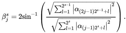
As shown in the Figure 1, β represents the Y-axis rotation angle, and αi is the ith element of the amplitude code. For a 2-qubit circuit, a 4-dimensional feature vector is encoded. Amplitude encoding requires the feature vector to be normalized to unit norm by sample, which results in different normalization factors. Therefore, 3 informative features were used and were subsequently padded with a non-zero constant term of 0.01 to obtain a 4-dimensional vector, which would ultimately bear information on the normalization factor.
4.2. Ansatz Circuit Construction: Used to Train Parameters in Parameterized Quantum Gates
Initializing the quantum circuit instance, set the circuit depth and the number of qubits. At each depth level, multiple rotation gates (such as RZ, RY) are applied to each qubit, and entanglement between qubits is achieved through CNOT gates. The introduction of parameterized rotation operations enables the model to adapt to complex data patterns and capture nonlinear relationships of data.
As shown in the Figure 2, a parameterized entanglement circuit model is defined, which consists of 6 layers of unitary units, each of which has an arbitrary single qubit rotation (Rot gate) followed by a CNOT gate. The Rot gate is parameterized by 3 angle values ω, θ, and φ, and can be written as a function of Y-axis and Z-axis rotation RZ(ω)RY (θ)RZ(φ).
4.3. Measurement: For Detecting Measurement Values
Calculating the expected value of the Pauli Z operator acting on the 0th qubit and the 1st qubit. At this time, there are 2 Hamiltonians constructed, and the coefficients are all set to 1. If the 0th bit measurement value is larger, the sample will be classified into the class with label "0". Similarly, if the 1st bit measurement value is larger, the sample will be classified into the class with label "1". Through the training of the neural network, it is expected that the 0th bit measurement value of the sample with label "0" in the training sample is larger, and the 1st bit measurement value of the sample with label "1" is larger. Finally, this model is applied to predict the classification of new samples.
4.4. Model Training
We used the MindSpore framework (https://www.mindspore.cn/en) to create a quantum model and initializing the simulator to calculate the expected value. The expected value is used to optimize the model parameters during training.
“SoftmaxCrossEntropyWithLogits” in tensorflow is used as the loss calculation method, and the Adam optimizer is used to adjust the trainable parameters of the quantum neural network. Use “NumpySlicesDataset” in mindspore dataset to create a dataset and set the batch size to 5. Defining a callback function to monitor the accuracy during training, record the loss and the optimal balanced accuracy. Here Epoch=20, which means the model will perform a maximum of 20 complete iterations on the entire training dataset. Besides, an early stop strategy for balance accuracy (bACC) is set.
5. Prediction Results
The results of the Quantum Neural Network (QNN) evaluation indicate a balanced performance across various metrics. The test balanced accuracy (bACC) and the ROC-AUC both achieved a score of 0.71, suggesting effective classification capabilities. However, the precision varied significantly, with a score of 0.32 and a higher value of 0.93 in a “0” and “1” respectively, indicating inconsistencies in the true positive rate. The recall remained consistent at 0.71, while the f1-score showed a range between 0.44 (for “0”) and 0.8 (for “1”), reflecting variability in the model's performance across different scenarios. Overall, while the QNN demonstrates potential, there are areas for improvement, particularly in precision and f1-score consistency (see Table 1 and Figure 3)
5. Discussion
5.1. Bias in Data Set Classification
A key issue is bias in data classification, which leads to poor predictions for minority classes, especially class "0". This is a common problem in classical machine learning, where imbalanced datasets cause models to favor the majority class. In QML, this issue is worsened by the early stage of quantum algorithms and hardware. Current quantum models, like quantum support vector machines (QSVMs) or quantum neural networks (QNNs), are experimental and struggle with imbalanced data. Classical techniques like oversampling or synthetic data generation (e.g., SMOTE) are not yet optimized for quantum systems, and quantum noise further complicates fair classification.
To cope with this problem, it may involve solutions such as developing quantum-specific techniques for data augmentation to balance datasets effectively. Additionally, hybrid approaches that combine classical pre-processing with quantum algorithms can help reduce bias. Furthermore, designing quantum algorithms that are robust to class imbalance is crucial; this could include strategies that penalize the misclassification of minority classes to ensure fairer outcomes.
5.2. Difficulty in Demonstration of Quantum Speedup
Another challenge is demonstrating quantum speedup on classical computers. Quantum computers are theorized to offer exponential speedups for tasks like factorization and optimization, but simulating quantum systems on classical hardware is computationally expensive and doesn’t reflect true quantum speedup. Simulating quantum systems with n qubits requires 2^n complex numbers, making large-scale simulations impractical.
Perhaps collaboration with providers such as IBM, Google, and Rigetti to gain access to quantum hardware for conducting experiments on real quantum processors can offer solution. Additionally, the development of hybrid algorithms that leverage both classical and quantum systems can help partially demonstrate quantum speedup on classical hardware. Furthermore, establishing standardized benchmarks is essential for evaluating quantum machine learning performance, even in the absence of large-scale quantum hardware.
5.3. Quantum Hardware Limitations
Current quantum hardware faces challenges like short qubit coherence times, low gate fidelity, and high error rates. These limitations affect the performance and scalability of QML models
Quantum algorithms need extensive circuit depths since computation errors accumulate over time. Modern error correction systems known as surface codes need substantial computing resources that prevent large-scale practical implementation. The restricted number of qubits creates a limit to the complexity of problems which quantum computers can solve.
The approach to reduce quantum computing noise impact involves developing error-mitigation methodologies while minimizing operational errors.
5.4. Integration with Classical Systems
The operations of quantum computers require complete integration with classical systems for managing data pre-processing together with control functions. It is important to have a seamless integration of quantum and classical systems that include hardware and software technologies; efficient communication networks and programming frameworks that combine the two computational arenas. Currently Qiskit (from IBM) and Cirq (from Google) are potential frameworks that aim to unite quantum and classical technologies. Creating middleware serves as a solution to establish reliable data exchange and synchronization and manage errors among different systems. Therefore the development of industry standards must be implemented to establish uniformity across quantum-classical interfaces in different platforms.
5.5. Future Directions
The advancement of Quantum Machine Learning (QML) requires future research to work on multiple essential areas. The research requires algorithmic progress to create resilient quantum algorithms that specifically operate for machine learning needs. Quantum error correction methods may further need to be improved to enhance smooth implementation, while new quantum state encoding approaches for classical data will enhance the quantum framework data utilization. The performance evaluation of QML against traditional methodologies requires established benchmarks to determine both practical and instrumental development. Interdisciplinary collaboration between quantum physicists and computer scientists as well as domain experts will strengthen multilateral learning and advance the quantum field.
6. Conclusion
Our study demonstrated a feasibility of using QML for radiomic predication. Research achievements in quantum computing will be possible through combined efforts between scientists and industry specialists and governmental personnel, although problems such as data bias, hardware limitation and system integration remain to be solved. Quantum technology is progressing in steps which will allow scientists to reach the complete potential of QML.
References
- Zeguendry A, Jarir Z, Quafafou M. Quantum Machine Learning: A Review and Case Studies. Vol. 25, Entropy. MDPI; 2023. [CrossRef]
- Wang Y, Liu J. A comprehensive review of Quantum Machine Learning: from NISQ to Fault Tolerance. 2024 Jan 20; Available from: http://arxiv.org/abs/2401.11351.
- Senokosov A, Sedykh A, Sagingalieva A, Kyriacou B, Melnikov A. Quantum machine learning for image classification. Mach Learn Sci Technol. 2024 Mar 1;5(1). [CrossRef]
- Tang FH, Fong YW, Yung SH, Wong CK, Tu CL, Chan MT. Radiomics-Clinical AI Model with Probability Weighted Strategy for Prognosis Prediction in Non-Small Cell Lung Cancer. Biomedicines [Internet]. 2023;11. Available from: https://api.semanticscholar.org/CorpusID:260220203.
- Tam SY, Tang FH, Chan MY, Lai HC, Cheung S. Prognosis Prediction in Head and Neck Squamous Cell Carcinoma by Radiomics and Clinical Information. Biomedicines [Internet]. 2024;12. Available from: https://api.semanticscholar.org/CorpusID:271446756.
- Munshi M, Gupta R, Jadav NK, Tanwar S, Nair A, Garg D. Quantum Machine Learning-based Lung Cancer Prediction Framework for Healthcare 4.0. 2024 Asia Pacific Conference on Innovation in Technology, APCIT 2024. 2024; [CrossRef]
- Preskill J. Quantum Computing in the NISQ era and beyond. 2018;
- Ciliberto C, Herbster M, Ialongo AD, Pontil M, Rocchetto A, Severini S, et al. Quantum machine learning: a classical perspective. Proceedings of the Royal Society A: Mathematical, Physical and Engineering Sciences [Internet]. 2017 Jul 26 [cited 2025 Feb 11];474(2209). Available from: http://arxiv.org/abs/1707.08561.
- Van Griethuysen JJM, Fedorov A, Parmar C, Hosny A, Aucoin N, Narayan V, et al. Computational radiomics system to decode the radiographic phenotype. Cancer Res. 2017; [CrossRef]
- Zwanenburg A, Vallières M, Abdalah MA, Aerts HJWL, Andrearczyk V, Apte A, et al. The image biomarker standardization initiative: Standardized quantitative radiomics for high-throughput image-based phenotyping. Radiology [Internet]. 2020 May 1 [cited 2024 Dec 27];295(2):328–38. Available from: https://pubs.rsna.org/doi/10.1148/radiol.2020191145.
Figure 1.
Encoder Circuit construction.
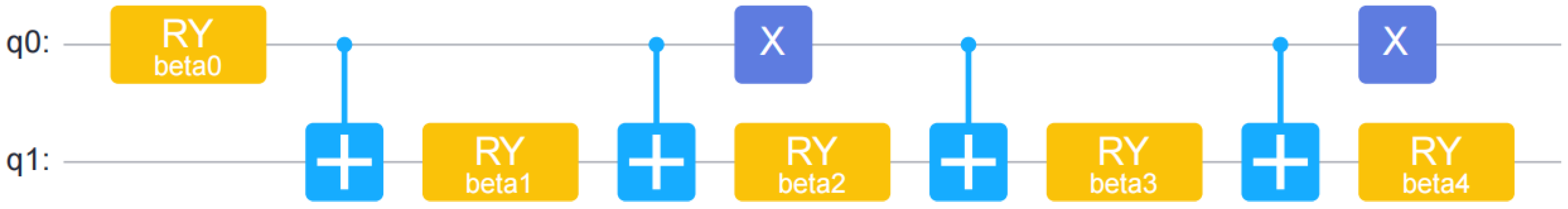
Figure 2.
Ansatz circuit.

Figure 3.
ROC curve of QNN model.


Table 1.
Result of QNN.
| QNN | ||
| Test | Prediction Outcome | Prediction Result |
| Test bACC | 0.71 | |
| Test ROC-AUC | 0.71 | |
| Test precision | 0 | 0.32 |
| 1 | 0.93 | |
| Test recall | 0 | 0.71 |
| 1 | 0.71 | |
| Test f1-score | 0 | 0.44 |
| 1 | 0.8 | |
Disclaimer/Publisher’s Note: The statements, opinions and data contained in all publications are solely those of the individual author(s) and contributor(s) and not of MDPI and/or the editor(s). MDPI and/or the editor(s) disclaim responsibility for any injury to people or property resulting from any ideas, methods, instructions or products referred to in the content. |
© 2025 by the authors. Licensee MDPI, Basel, Switzerland. This article is an open access article distributed under the terms and conditions of the Creative Commons Attribution (CC BY) license (http://creativecommons.org/licenses/by/4.0/).
Copyright: This open access article is published under a Creative Commons CC BY 4.0 license, which permit the free download, distribution, and reuse, provided that the author and preprint are cited in any reuse.


