Submitted:
01 April 2025
Posted:
02 April 2025
You are already at the latest version
Abstract
Geophysical and astrophysical flows are characterized by rapid rotation. Simulating these flows requires small timesteps to achieve stability and accuracy. Numerical stability can be greatly improved by implicit integration of the terms that are most responsible for destabilizing the numerical scheme. We have implemented an implicit treatment of the Coriolis force in a rotating spherical shell driven by a radial thermal gradient. We have modified the resulting timestepping code to carry out steady-state solving via Newton’s method, which has no time-stepping error. The implicit terms have the effect of preconditioning the linear systems, which can then be rapidly solved by a matrix-free Krylov method. We compute branches of rotating waves with azimuthal wavenumbers ranging from 4 to 12. As the Ekman number (the non-dimensionalized inverse rotation rate) decreases, the flows are increasingly axially independent and localized near the inner cylinder, in keeping with well-known theoretical predictions and previous experimental and numerical results. The advantage of the implicit over the explicit treatment also increases dramatically with decreasing Ek, reducing the cost of computation by as much as a factor of 10 for Ekman numbers of order 10−5. We carry out continuation in both Rayleigh and Ekman number and obtain interesting branches in which the drift velocity remains unchanged between pairs of saddle-node bifurcations.
Keywords:
rotating fluids
; Krylov methods
; preconditioning
; bifurcation
; rotating waves
MSC: 35B32; 37M20; 65F08; 65M70; 65N35; 65P30; 76E06; 76U60
1. Introduction
Convection in a rotating spherical annulus is a classic configuration in hydrodynamics [1,2,3,4]. At moderate parameter values, it provides beautiful and deep examples of symmetry-breaking bifurcations leading to complex patterns, e.g. [5,6,7,8,9,10,11,12,13]. At more extreme parameter values, the turbulent flow it engenders is among the fundamental processes in planets and stars, e.g. [14,15]. We do not attempt here to survey the considerable literature devoted to this configuration nor to derive new results in either of these well-studied regimes. Instead we describe the implementation and capabilities of a pair of numerical codes – two drivers relying on a common set of subroutines – that incorporate an implicit treatment of the Coriolis force to carry out both timestepping and also continuation via Newtons’s method.
We will illustrate, test, and compare the codes on the simplest convective states, which are rotating waves (RW). Their appearance at onset is a mathematical consequence of the invariance of the system under azimuthal rotation, but not under azimuthal reflection, which is broken by the rotation of the system [16,17,18]. We have carried out numerical continuation in both Rayleigh and Ekman numbers. We have found interesting examples of branches which contain saddle-node bifurcations separating plateaus in drift frequency.
Our numerical algorithm uses the basic framework described in [11,12,13,19] and the spherical harmonic library of [20]. The research which is closest to ours is that of [21,22,23,24], who, like us, have carried out implicit timestepping and continuation for convection in a rotating spherical shell and explored various interesting parameter regimes. There are a number of differences between our continuation method and theirs, some of which have been analyzed in [25] and which we will discuss after we have described our numerical methods. We mention here also that [14,15,26] have implemented implicit Coriolis timestepping.
2. Physical Description
2.1. Governing Equations
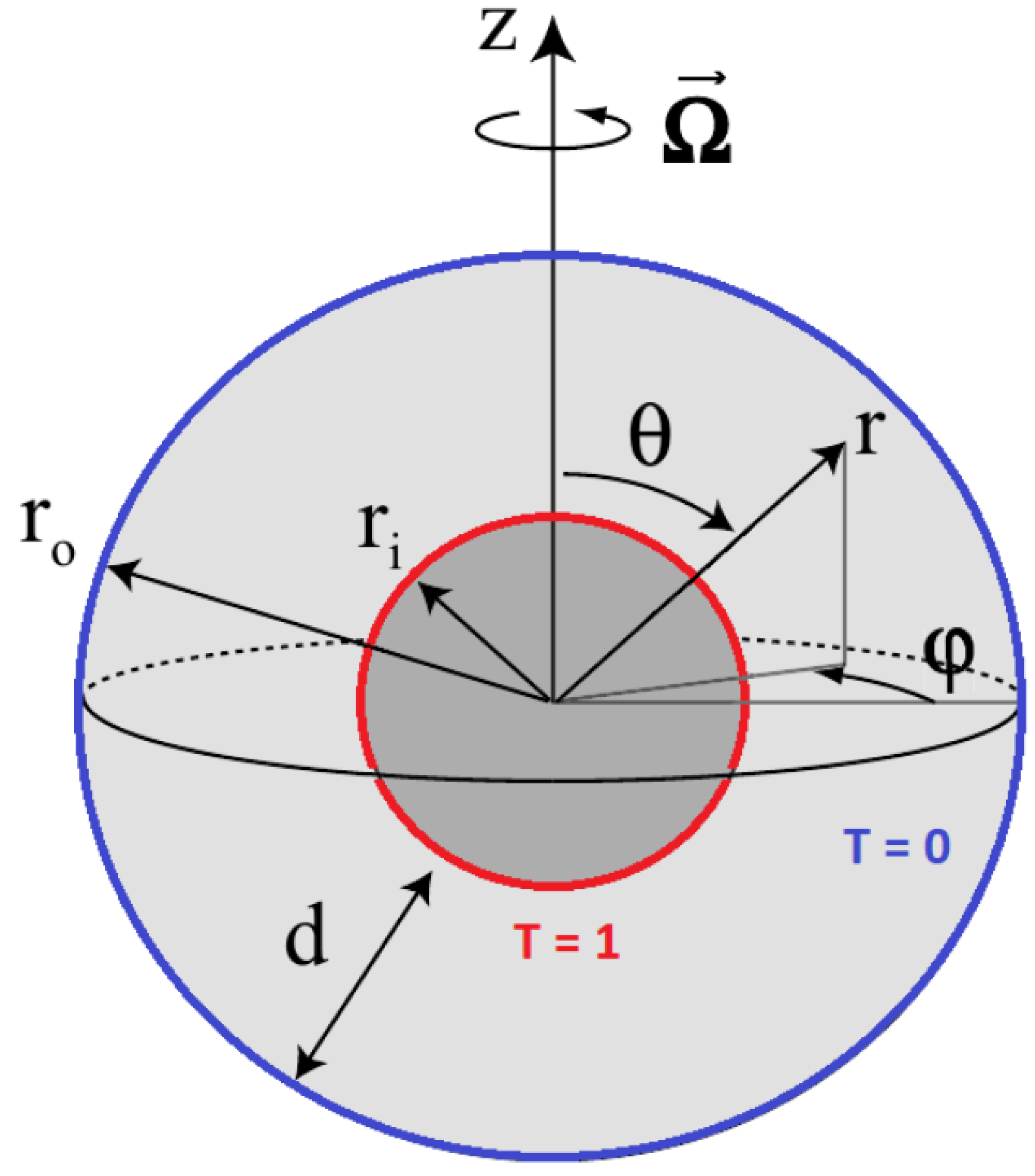
We study classical Rayleigh-Bénard convection in a spherical fluid shell rotating with constant angular velocity about the z axis. The shell is heated from within by imposing a temperature difference between the inner and outer spherical boundaries. Lengths are non-dimensionalized with the gap size d, so that the dimensionless outer and inner radii are and , respectively. The aspect ratio can be specified via or via . Time is scaled by the viscous diffusion time , where is the kinematic viscosity and the flow velocity is scaled by the viscous diffusion velocity . Measuring temperature from a reference temperature at which the mass density is , we nondimensionalize pressure by , and temperature by .
Figure 1.
Geometry. The domain is the spherical annulus between an inner and outer sphere of radius and whose temperatures are fixed at and . Both spheres rotate around the z axis with angular velocity .
Figure 1.
Geometry. The domain is the spherical annulus between an inner and outer sphere of radius and whose temperatures are fixed at and . Both spheres rotate around the z axis with angular velocity .
The gravitational acceleration g is assumed to be proportional to the distance r from the center of the sphere (as is the case for the self-gravity in the interior of a spherical body with constant mass density) and is thus of the form , where is the acceleration at radius . The resulting nondimensional Boussinesq equations read:
The centrifugal acceleration and a gradient part of the acceleration due to buoyancy have been included in the pressure gradient. The non-dimensional parameters used in (1a) above are the Ekman, Prandtl, and Rayleigh numbers:
where is the thermal diffusivity and is the thermal expansion coefficient. The Rayleigh number used here is adapted to the rotating case and is related to the conventional thermal Rayleigh number by
In what follows, we will denote merely by . No-slip and fixed temperature boundary conditions are applied at the inner and outer radii:
and the conductive solution is:
Following the benchmark study [27], we set the Prandtl number to and the radii to and (so that ) throughout the investigation and we will vary and .
2.2. Overview
The first states to appear at the onset of convection are rotating waves. We denote these by where M is the azimuthal wavenumber of the rotating wave. Figure 2(a) and Figure 2(b), modeled on those in [12], display properties of some of these rotating wave solutions for . Four traveling waves are shown, with azimuthal wavenumber from to . At , is the first in Rayleigh number to bifurcate, and therefore it is the only one which is stable at onset. The drift frequency, i.e. the frequency relative to the imposed frequency , decreases as increases, from prograde (faster than ) to retrograde (slower than ). These results were obtained via timestepping simulations starting from initial conditions of the form .
Figure 3 shows the qualitative evolution of the rotating waves as is decreased from to : the flow is increasingly stronger near the inner sphere and the azimuthal wavenumber increases. These two properties are related. Each half-wave tends to occupy an equal length in radius () and in circumference (), leading to . With decreasing , the radius decreases [28] and so M increases. The appeared naturally when performing timestepping simulations from an initial condition of the form at , as did the at . This result was then used as input for a path-following computation to obtain the data at . The same techniques were applied to obtain the data at starting from the existing results of the same rotating wave at .
3. Numerical Methods
3.1. Spatial Representation
The velocity is decomposed into toroidal and poloidal potentials e and f such that
These and the temperature are expanded in spherical harmonics and Chebyshev polynomials . of the shifted radius .
To carry out transformations to and from the spherical harmonic space, we use the SHTns library [20]. This is a highly efficient code that uses the FFTW library to perform fast transformations to and from Fourier space, and the recursion relations presented in [29] for optimized computation of the associated Legendre polynomials. Although the library allows for multithreaded computations as well as GPU offloading, these capabilities were not used in the present work.
Dealiasing in the r direction is carried out according to the rule, whereas in the and directions, it is performed by SHTns. To achieve this, the library determines a suitable number of physical points based on the non-linear order of the equations to be solved (two in this case) with the aim of maximizing the efficiency of the FFT algorithm. Moreover, for solutions which have azimuthal periodicity , we restrict our calculations to a segment of the sphere , or, equivalently, to those which have Fourier expansions containing only multiples of the wavenumber M; this is easily implemented using options in SHTns. Lastly, we will denote the physical points in and as and , respectively. The resolutions used will be given in the captions of each of the figures.
The radial component of the curl and of the double curl of equation (1a) are taken, leading to:
where
Equations (8) and (9) are decoupled in ℓ, m and in potential (e vs f), and so its discrete version involves a block-diagonal matrix with blocks that are each , as in Figure 5(a).
The temperature field is also expanded in Chebyshev polynomials and spherical harmonics like (7). Its evolution is governed by the discretized form of (1b).
3.2. Implicit Coriolis Integration
To carry out implicit integration of the Coriolis term, we include the Coriolis force in the left-hand-side and remove it from , leading to:
where
The recursion relations of the Legendre polynomials
together with
can be used to transform (11a) and (11b) into:
In contrast with (8)-(9), equations (15a)-(15b) are coupled in several ways:
- The spectral coefficients and both appear in both equations.
- While each m can be treated independently, components ℓ, , and are coupled.
- The real and imaginary parts of and are coupled via the imaginary coefficient .
However, two decoupled classes of coefficients appear, one class containing coefficients with odd l for and even l for and a second class with the opposite property. For example the real component of is coupled to its imaginary component and to the real parts of . The sums in (15a) and (15b) are represented by block pentadiagonal matrices, as illustrated in Figure 5(b).
3.3. Newton Method
We represent our system of governing equations schematically by
For our problem, corresponds to the poloidal and toroidal fields e and f and the temperature T. For explicit or implicit Coriolis integration, corresponds to the right-hand-sides of (8)-(9) or of (15a)-(15b), respectively. corresponds to minus the left-hand-sides of the same equations with the time derivative omitted. (The correspondence is imperfect, since does not act directly on .)
We represent our timestepping code schematically by the following implicit-explicit Euler method:
where is linear (though need not be nonlinear). Steady states are solutions to
or, alternatively
where is a solution to the continuous-time differential equation (16). Surprisingly, (19) is also a criterion for stationarity when is calculated via the time-stepping scheme (17) for any value of , as can be seen from
Thus and so roots of of (18) can be found by computing roots of , which is simply the difference between two large consecutive timesteps. Note that (20) does not use Taylor series; can be of any size. Indeed, for large, acts as a preconditioner (approximate inverse) for , whose poor conditioning is due to that of . Typically, for Newton solving we use .
Finding the roots of (20) via Newton’s method requires the solution of the linear system
where is the current estimate and is the Jacobian of evaluated at , with substituted for in (17). For example, if contains , this term becomes in , as well as in the operators and .
We solve (21) using a Krylov method such as GMRES [30]. In such matrix-free methods, one need only provide the right-hand-side for the current estimate, and a routine which carries out the action of on any vector . The computational cost of a Newton step can be measured by the number of such actions (i.e. GMRES iterations) taken by the Krylov method, since the right-hand-side remains constant throughout the step. The number of GMRES iterations required is low if is well-conditioned; it is for this reason that we take large. Once the decrement is determined by solving (21), it is subtracted from to form an improved estimate. We accept as the decrement if the linear system (21) is solved by GMRES to relative accuracy . For Newton’s method, we accept as a steady state, i.e. a solution to (19), if .
This method [11,12,13,25,31,32] has been called Stokes preconditioning because the linear operator which is integrated implicitly in (17) is usually the viscous term that occurs in Stokes equation. However, it is beneficial to include as many possible other terms in , as long as they are linear and can be inverted directly. It is for the reason that we have included the Coriolis force in , as described in Section 3.2. In Section 5, we will compare the cost of computations using Newton’s method with implicit vs. explicit Coriolis integration for various values of the Ekman number by comparing the number of GMRES iterations necessary for each.
3.4. Traveling Waves
Newton’s method can also be used to compute traveling waves in the same way. Azimuthal rotating waves satisfy , where C is an unknown wavespeed. Thus, . Substituting into (16) and dropping the tildes leads to
The explicit portion of the timestep is augmented to include as well as :
If is expressed in terms of spherical harmonics in which the dependence is trigonometric, the action of on a Fourier component is merely .
Expanding around and truncating at first order leads to the linear system that must be solved for the decrements :
The preconditioner remains with large , since continues to be responsible for the large condition number of (25).
An additional equation must be added to the system to compensate for the additional unknown. We choose a phase condition, more specifically we require the imaginary part of a single component (temperature, toroidal or poloidal field; radial and angular and azimuthal mode) of be zero, i.e. that the corresponding phase component (whose index we shall call J) of remains unchanged.
This simple choice suggests a trick for retaining the size of the unknown rather than using augmented fields, since is no longer an unknown. The routine which acts on is defined such that c is stored in . At the beginning of an action, c is extracted, is set to zero, and the explicit part of the action on is carried out. Then we multiply the stored value of by c and add the result to the explicit part of the action. When the Krylov method converges and returns , we must again extract c from , after which is set to zero. Effectively, although C and c have been added to the unknowns for the Newton method and for the linear equation, and are no longer unknowns.
3.5. Continuation
We compute solutions along a branch via Newton’s method as described above. We do not impose additional equations, such as requiring a new solution along the branch to be a certain distance from a prior solution or that the increment along the branch must be perpendicular to some direction. Therefore the only additional ingredients that must be introduced to discuss continuation are the choice of initial estimate for each solution along the branch and the parameters that are prescribed for the Newton iteration.
If the continuation is in Rayleigh number, we increment or decrement this parameter according to the number of Newton iterations required for convergence in the previous step as follows [33]:
where , denote the Rayleigh numbers used in the two previous continuation steps, is the increment or decrement, and is defined by:
is the target number of Newton iterations. If , then remains unchanged, whereas it is reduced (increased) if . The choice of is guided by two considerations. The first is the level of sampling desired along the branch. The second is economy: a smaller value of will engender more values of , but each calculation will be faster. For our computations we fixed to be between 4 and 6.
To choose an initial estimate for the next solution along a branch at , first-order and even zero-th order extrapolation (i.e. using just the previously computed field) can be used to follow a smooth and monotonically varying branch. However, quadratic extrapolation is essential for going around turning points. Lagrange interpolation uses the three previous Rayleigh numbers , , and the new Rayleigh number from (27) to determine coefficients such that
after which we set
to form a new estimate of the solution. Newton iterations are then used to refine until the norm of (22) is . This procedure requires saving the three previous solution vectors and Rayleigh numbers.
3.6. Turning Points
We now turn to the more complicated matter of extrapolating near saddle-node bifurcations, at which ceases to be a single-valued function of . The code detects that the current step is in the vicinity of a turning point by comparing relative changes between the solution vector , and the Rayleigh number, i.e. we compare
where J is the index denoting the element of the solution vector of highest absolute value and is a constant factor that makes the two magnitudes comparable. For our computations we fixed this constant to be between 10 and 100.
Since the normal form of a saddle-node bifurcation at is , dependent variables (x, ) vary like the square root of the control parameter (, ) near a turning point. Consequently, as the current solution approaches a turning point, the relative difference increases until it is greater than that of . It is at this stage that the code switches to extrapolating quadratically, using the component as the independent variable instead of the Rayleigh number. This allows to change sign and the continuation to go around the turning point. We replace (27) and (29) by analogous equations in to determine and , and then replace (29) and (30) by
to set the estimate of the new solution. Note that we have only changed the method of determining the initial guess. remains fixed to during the Newton step, while all the elements of are allowed to vary.
Continuation follows in this manner until eventually exceeds , at which point the code switches back to using the Rayleigh number as the independent variable. The parameter can be obtained by analyzing the behaviour of the continuation near a turning point. Indeed, if is too large, then the code will continue to use as the independent variable past the point at which there is no solution for the next continuation step, and Newton’s method will not converge. Should this situation arise, the continuation can be restarted at the last converged solution using a suitably reduced value of .
4. Branch Following
4.1. Continuation in Rayleigh Number
We used the continuation code to compute branches of rotating waves. As previously explained, to search for solutions having an M azimuthal periodicity we perform our computations to a fraction of the domain given by . The solutions are computed independently of their stability; most of the solutions we compute are unstable, either within the restricted domain , or to instabilities which break this restriction such as rotating waves with a different M.
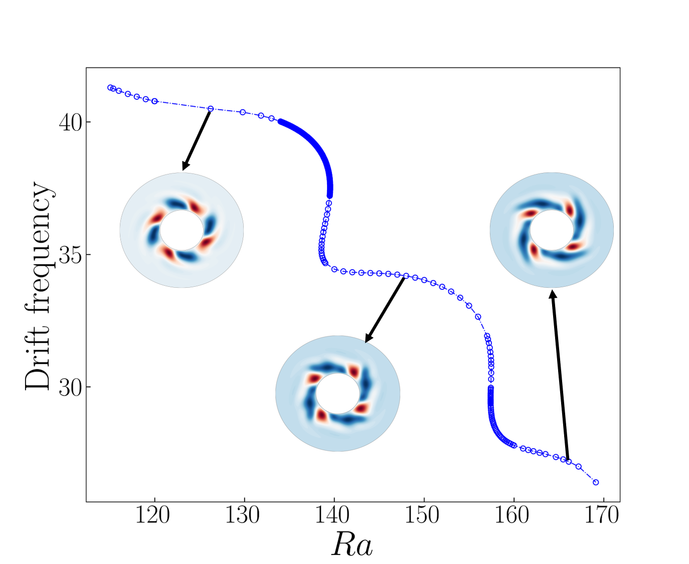
Fixing the Ekman number, we carried out continuation in Rayleigh number . Most of the branches that we computed showed no unusual features, varying smoothly and monotonically down to their threshold at a supercritical Hopf bifurcation. However, a few branches presented some interesting non-monotonic behavior, which we show in order to display the capacities of our code. Figure 6 tracks the Rayleigh-number dependence of the branch for . This branch consists of three smooth regions that are separated from one another by short intervals which each contain two saddle-node bifurcations and rapid changes in drift frequency. In order to focus in on these intervals, we have computed branches at slightly higher and lower Ekman numbers in Figure 7 and Figure 8. Each of these branches contains a single interval of rapid change. We also computed an branch for , shown in Figure 9. Indeed, for this value of , rotating waves with azimuthal wavenumber 8 are more appropriate, i.e. more likely to be stable. This branch also contains a plateau in drift frequency adjacent to a short interval at of rapid change delimited by two saddle-node bifurcations. These rapid rises and plateaus in drift frequency should have a physical or phenomenological explanation, but we have not been able to find one.
4.2. Continuation in Ekman Number and in Resolution
We adapted our method to follow branches in Ekman number, varying on a logarithmic scale. We replace with in (27) as follows:
where the computation of remains as in equation (28). In this case, we used for all of the simulations. Furthermore, in order to go around turning points, we now compare and , where we chose between 400 and 500.
Apart from these minor changes, there are several major differences between performing continuation in Ekman and Rayleigh numbers. The first is that the matrices that represent the left-hand-sides of (8)-(9) or (11a)-(11b) must be recomputed every time a new value of is chosen. Indeed, while the Rayleigh number only appears in the right hand side of these equations, is also present in the diffusion terms, which are treated implicitly regardless of how the Coriolis term is treated. This means that extra work must be done at the beginning of every continuation step.
Secondly, as the Ekman number is decreased, the critical Rayleigh number for onset of convection increases. That is, rotation stabilizes the configuration against convection. A classic result is that the critical value of the usual thermal Rayleigh number varies like , so that the critical value of our Rayleigh number varies like . Therefore, instead of keeping fixed as we vary , we have kept fixed by increasing every time we decrease .
Third, as the simulation ventures towards lower Ekman numbers, the fields require a higher resolution. This is clearly seen from the visualizations in Figure 3, which show that the radial extent and azimuthal wavelength decrease with . To achieve this, grid refinement is introduced in the code such that the spectral resolution is increased by 20% whenever under-resolution is detected in the Chebyshev or the spherical harmonic modes. This is done by introducing a threshold for the amplitude ratio between the mode of highest absolute value and of highest wavenumber. When this ratio exceeds the threshold, the code calls a grid refinement subroutine which first deallocates the previous grid, then creates a new one using the new resolution and finally represents the fields from the last continuation step on this new grid by filling in the new modes with zero. This last step is then recomputed with the new resolution and path following continues as intended. In our computations we chose the under-resolution threshold to be between and .
Figure 10 shows the result of continuation in . Because the convective threshold obeys a scaling law [2], we fixed to be proportional to so as to remain at approximately the same distance from the convective threshold. This branch showed three coexisting solutions over the range . Our grid refinement algorithm increased the resolution in r by about 20% and by 50% in and . We emphasize that most continuations showed monotonic behavior and we have chosen deliberately to present those that did not.
5. Timing Comparisons
Newton’s method is very fast, typically requiring 3-10 iterations. The bottleneck in applying Newton’s method to systems of partial differential equations is always the solution of the linear systems. In our case, this is quantified by the total number of GMRES iterations necessary to compute a new state along the branch. We find that the number of iterations depends on the Ekman number, but is fairly independent of the Rayleigh number. We therefore average the number of GMRES iterations over all the points computed in a branch for a fixed Ekman number. We do this for the Newton method with both implicit and explicit Coriolis to produce the curves in Figure 11, Figure 12, and Figure 13.
Measuring the economy realized in timestepping is more problematic. Because explicit integration effectively approximates a decaying exponential by a polynomial, it displays artificial temporal divergence if the timestep is too large. Because implicit integration instead approximates the exponential by a decaying rational function, the timestep is not constrained by stability. The timestep is, however, still constrained by accuracy. A particularly demanding criterion for judging accuracy is the wavespeed [34]. We compute the relative errors in wavespeeds , where is obtained from Newton’s method and hence has no timestepping error. Figure 14 presents the relative errors as a function of and , with the other parameters set to the values below the figure. The errors obtained from the explicit and implicit methods are the same for the same value of . For each , there is a minimum above which the explicit simulation diverges in time, but the implicit simulation still yields a solution with an error that is less than 5%. This value of is indicated in Figure 14 by the left endpoint of an arrow for each Ekman number. But eventually, is so large that the result of the implicit method can even be qualitatively incorrect. As an upper limit for the implicit method, we choose that the relative error on must be less than 5%. The limiting values of large are indicated as the right endpoints of the arrows in Figure 14 and in Table 1. Hence, for each , there is a range of -values that can be used only for implicit timestepping and whose error does not exceed . These ranges are given in Table 1. Although these results are specific to the parameter values and flows that we have simulated, they suggest that implicit Coriolis integration can be orders of magnitude faster, enabling the simulation of convection in a spherical annulus at low Ekman numbers.
6. Discussion
We have developed a pair of codes for simulating thermal convection in a rotating spherical fluid shell that rely on an implicit treatment of the Coriolis force. The numerical cost of this improvement is quite manageable: the block diagonal matrix systems which arise from implicit treatment of the diffusive terms must be replaced by block pentadiagonal matrix systems, which can still be solved by block banded LU decomposition and backsolving. Once implemented in a timestepping code, implicit integration with a very large pseudo-timestep () can be leveraged to precondition the large linear systems that are the core of Newton’s method. When only the diffusive terms are treated implicitly, this is known as Stokes preconditioning [11,12,13,25,31,32]; we could call the method developed here Stokes-and-Coriolis preconditioning.
We have demonstrated this method’s capabilities by carrying out continuation in Rayleigh number at various values of the Ekman number on the order of for rotating waves with azimuthal wavenumbers 4, 8, and 12. We have found several intriguing examples of such branches contain plateaus in drift frequency, separated by intervals of rapid change delimited by pairs of saddle-node bifurcations. The physical, or at least phenomenological, reasons for these properties remain to be discovered. We have also implemented continuation in Ekman number, spaced logarithmically, in which we automatically measure and increase the resolution as needed. We are unaware of any previous examples of continuation in Ekman number or with automatic resolution adjustment in the literature.
We have measured the economy that is realized by implicit treatment of the Coriolis force. For Newton’s method, the advantage of the implicit over the explicit treatment is dramatic. For example, the explicit algorithm takes 20 times as many GMRES iterations (and hence 20 times as much CPU time) as the implicit method to compute states on the branch at . For lower Ekman numbers, the explicit method takes an unmanageable number of GMRES iterations, making it impossible to use in practice.
For timestepping, the advantage of the implicit over the explicit treatment is equally spectacular. For computing rotating waves at , the implicit algorithm can reasonably use timesteps that are 200 times past the temporal stability limit, meaning that simulations in this regime can be 200 times faster than if an explicit method were used.
We now describe the differences between Stokes preconditioning and the method used in [21,22,23,24] for convection in rotating spheres, as well as by [35,36,37,38] for other hydrodynamic problems. These authors seek steady states or traveling waves as roots of , where is computed from in the usual manner by carrying out many timesteps, each with a small ; we call this the integration method. In contrast, although equations (19)-(20) would seem to imply that we too seek roots of , this is not at all the case. In the Stokes preconditioning method, we compute from by carrying out a single very large implicit-explicit Euler timestep (17), with a timestep that is so large that the difference no longer approximates the time derivative. Via equation (20), it turns out that this difference is a preconditioned version of the operator whose roots are sought by our method, namely , preconditioned by . Both methods solve the linear systems that are the core of Newton’s method via GMRES, which relies on repeated actions of the Jacobian. For the integration method, the action of the Jacobian consists of integrating the linearized equations via many small timesteps, while for us it consists taking a single large linearized timestep. Here, there is a trade-off. Despite the preconditioning displayed by (20), the Jacobian resulting from Stokes preconditioning is less well conditioned than that which results from taking many small linearized timesteps, and so more Jacobian actions are required for GMRES to converge to a solution of the linear system (21). However, each action costs less, since it consists of only a single timestep. This trade-off – number of actions vs. timesteps per action – can be quantified via the total number of timesteps required to compute a steady state or travelling wave. For wall-bounded shear flows in the transitional regime, we have found that the Stokes preconditioning method is faster than the integration method by a factor of 11 for plane Couette flow and by a factor of 35 for pipe flow; see [25] for details. We have not carried out a timing comparison of the integration and the Stokes preconditioning method for convection in rotating spheres.
Although the Stokes preconditioning method is faster the integration method is more general. The Stokes preconditioning method is only capable of computing steady states or traveling waves, while the integration method can compute periodic orbits of all kinds, including, for example modulated rotating waves or pulsing states.
A specific difference between our implementation of implicit Coriolis integration and that of [21,22,23,24,28,39] is that we solve the linear systems arising from implicit treatment of the diffusive and Coriolis terms directly via block pentadiagonal LU decomposition and backsolving, whereas [21,22,23,24,28,39] use Krylov methods to solve these systems. Time-integration using explicit, implicit and semi-implicit treatment of the Coriolis term is compared by [39]. Our strategy is to solve linear systems directly as much as possible and to resort to Krylov only to invert the full Jacobian.
One might wonder about the applicability of this achievement to geophysical and astrophysical research. Small Ekman numbers, like large Reynolds numbers, are associated with chaos and turbulence, not with the regularity and periodicity of traveling waves, which moreover are almost invariably unstable. The Boussinesq and Navier-Stokes equations generally contain a very large number of solution branches, most of them partly or completely unstable [e.g., 33,36–38,40–42]. This profusion of states, sometimes called Exact Coherent Structures, has become the focus of extensive research, motivated by the idea [43,44] that turbulence could be viewed from a dynamical systems perspective as a collection of trajectories ricocheting between periodic orbits along their unstable directions, a kind of deterministic analogue of ergodic theory.
We now turn to the relevance of implicit Coriolis timestepping for geophysics. Implicit Coriolis timestepping not only speeds up calculations of stable and realistic flows, it also allows us to take much larger timesteps that yield inaccurate results. Constraints on timesteps (whether for stability or accuracy) arise from different physical forces. In rapidly rotating fluids, the Coriolis force generates inertial waves, which have a large range of frequencies and are continually generated and damped. Using a timestep that greatly exceeds the constraint for resolving inertial waves can be considered analogous to using the incompressible Navier-Stokes equations, which deliberately neglect the high-frequency sound waves [14,15].
Acknowledgments
We thank Adrian van Kan and Benjamin Favier for helpful discussions.
Author Contributions
The results were obtained by JCGS. FF provided discussions and additional results. The program was written successively by AR, CR and JCGS. The idea was suggested by LST and the paper was written by LST and JCGS.
Funding
The calculations for this work were performed using high performance computing resources provided by the Grand Equipement National de Calcul Intensif (GENCI) at the Institut du Développement et des Ressources en Informatique Scientifique (IDRIS, CNRS) through Grant No. A0162A01119.
References
- Chandrasekhar, S. Hydrodynamic and hydromagnetic stability; Oxford Univ. Press, 1961.
- Busse, F. Thermal instabilities in rapidly rotating systems. J. Fluid Mech. 1970, 44, 441–460. [Google Scholar] [CrossRef]
- Zhang, K.K.; Busse, F.H. On the onset of convection in rotating spherical shells. Geophys. Astrophys. Fluid Dyn. 1987, 39, 119–147. [Google Scholar] [CrossRef]
- Dormy, E.; Soward, A.; Jones, C.; Jault, D.; Cardin, P. The onset of thermal convection in rotating spherical shells. J. Fluid Mech. 2004, 501, 43–70. [Google Scholar] [CrossRef]
- Geiger, G.; Busse, F. On the onset of thermal convection in slowly rotating fluid shells. Geophys. Astrophys. Fluid Dyn. 1981, 18, 147–156. [Google Scholar] [CrossRef]
- Ardes, M.; Busse, F.; Wicht, J. Thermal convection in rotating spherical shells. Phys. Earth Planet. Inter. 1997, 99, 55–67. [Google Scholar] [CrossRef]
- Kitauchi, H.; Araki, K.; Kida, S. Flow structure of thermal convection in a rotating spherical shell. Nonlinearity 1997, 10, 885–904. [Google Scholar] [CrossRef]
- Simitev, R.; Busse, F. Patterns of convection in rotating spherical shells. New J. Phys. 2003, 5, 97. [Google Scholar] [CrossRef]
- Al-Shamali, F.; Heimpel, M.; Aurnou, J. Varying the spherical shell geometry in rotating thermal convection. Geophys. Astrophys. Fluid Dyn. 2004, 98, 153–169. [Google Scholar] [CrossRef]
- Kimura, K.; Takehiro, S.I.; Yamada, M. Stability and bifurcation diagram of Boussinesq thermal convection in a moderately rotating spherical shell. Phys. Fluids 2011, 23, 074101. [Google Scholar] [CrossRef]
- Feudel, F.; Bergemann, K.; Tuckerman, L.S.; Egbers, C.; Futterer, B.; Gellert, M.; Hollerbach, R. Convection patterns in a spherical fluid shell. Phys. Rev. E 2011, 83, 046304. [Google Scholar] [CrossRef]
- Feudel, F.; Seehafer, N.; Tuckerman, L.S.; Gellert, M. Multistability in rotating spherical shell convection. Phys. Rev. E 2013, 87, 023021. [Google Scholar] [CrossRef] [PubMed]
- Feudel, F.; Tuckerman, L.S.; Gellert, M.; Seehafer, N. Bifurcations of rotating waves in rotating spherical shell convection. Phys. Rev. E 2015, 92, 053015. [Google Scholar] [CrossRef] [PubMed]
- van Kan, A.; Julien, K.; Miquel, B.; Knobloch, E. Bridging the Rossby number gap in rapidly rotating thermal convection. arXiv preprint arXiv:2409.08536, 2024; arXiv:2409.08536 2024. [Google Scholar]
- Julien, K.; van Kan, A.; Miquel, B.; Knobloch, E.; Vasil, G. Rescaled Equations of Fluid Motion for Well-Conditioned Direct Numerical Simulations of Rapidly Rotating Convection. arXiv preprint arXiv:2410.02702, 2024; arXiv:2410.02702 2024. [Google Scholar]
- Ruelle, D. Bifurcations in the presence of a symmetry group. Arch. Rat. Mech. Anal. 1973, 51, 136–152. [Google Scholar] [CrossRef]
- Ecke, R.; Zhong, F.; Knobloch, E. Hopf bifurcation with broken reflection symmetry in rotating Rayleigh-Bénard convection. Europhysics Letters 1992, 19, 177. [Google Scholar] [CrossRef]
- Chossat, P.; Lauterbach, R. Methods in Equivariant Bifurcations and Dynamical Systems; World Scientific: Singapore, 2000. [Google Scholar]
- Hollerbach, R. A spectral solution of the magneto-convection equations in spherical geometry. Int. J Numer. Methods Fluids 2000, 32, 773–797. [Google Scholar] [CrossRef]
- Schaeffer, N. Efficient spherical harmonic transforms aimed at pseudospectral numerical simulations. Geochem. Geophys. Geosyst. 2013, 14, 751–758. [Google Scholar] [CrossRef]
- Sánchez, J.; Net, M.; Garcıa-Archilla, B.; Simó, C. Newton–Krylov continuation of periodic orbits for Navier–Stokes flows. J. Comput. Phys. 2004, 201, 13–33. [Google Scholar] [CrossRef]
- Garcia, F.; Sánchez, J.; Net, M. Antisymmetric Polar Modes of Thermal Convection in Rotating Spherical Fluid Shells at High Taylor Numbers. Phys. Rev. Lett. 2008, 101, 194501. [Google Scholar] [CrossRef]
- Sánchez, J.; Garcia, F.; Net, M. Computation of azimuthal waves and their stability in thermal convection in rotating spherical shells with application to the study of a double-Hopf bifurcation. Phys. Rev. E 2013, 87, 033014. [Google Scholar] [CrossRef]
- Garcia, F.; Net, M.; Sánchez, J. Continuation and stability of convective modulated rotating waves in spherical shells. Phys. Rev. E 2016, 93, 013119. [Google Scholar] [CrossRef]
- Tuckerman, L.S.; Langham, J.; Willis, A. Order-of-magnitude speedup for steady states and traveling waves via Stokes preconditioning in Channelflow and Openpipeflow. In Computational Modelling of Bifurcations and Instabilities in Fluid Dynamics; Springer, 2018; pp. 3–31.
- Marti, P.; Calkins, M.; Julien, K. A computationally efficient spectral method for modeling core dynamics. Geochemistry, Geophysics, Geosystems 2016, 17, 3031–3053. [Google Scholar] [CrossRef]
- Cardin, P.; Dormy, E.; Gibbons, S.; Glatzmaier, G.; Honkura, Y.; Jones, C.; Kono, M.; Matsushima, M. A numerical dynamo benchmark. Phys. Earth Planet. Inter. 2001, 128, 25–34. [Google Scholar]
- Garcia, F.; Sánchez, J.; Dormy, E.; Net, M. Oscillatory Convection in Rotating Spherical Shells: Low Prandtl Number and Non-Slip Boundary Conditions. SIAM Journal on Applied Dynamical Systems 2015, 14, 1787–1807. [Google Scholar] [CrossRef]
- Ishioka, K. A New Recurrence Formula for Efficient Computation of Spherical Harmonic Transform. Journal of the Meteorological Society of Japan 2018, 96, 241–249. [Google Scholar] [CrossRef]
- Saad, Y.; Schultz, M.H. GMRES: A generalized minimal residual algorithm for solving nonsymmetric linear systems. SIAM J. Sci. and Stat. Comput. 1986, 7, 856–869. [Google Scholar] [CrossRef]
- Tuckerman, L.S. Steady-state solving via Stokes preconditioning; recursion relations for elliptic operators. In Proceedings of the 11th Int. Conf. Num. Meth. Fluid Dyn. Springer, 1989, pp. 573–577.
- Mercader, I.; Batiste, O.; Alonso, A. Continuation of travelling-wave solutions of the Navier–Stokes equations. Int. J. Num. Meth. Fluids 2006, 52, 707–721. [Google Scholar] [CrossRef]
- Borońska, K.; Tuckerman, L.S. Extreme multiplicity in cylindrical Rayleigh-Bénard convection. II. Bifurcation diagram and symmetry classification. Phys. Rev. E 2010, 81, 036321. [Google Scholar] [CrossRef]
- Marcus, P.S. Simulation of Taylor-Couette flow. Part 1. Numerical methods and comparison with experiment. Journal of Fluid Mechanics 1984, 146, 45–64. [Google Scholar] [CrossRef]
- Duguet, Y.; Pringle, C.C.; Kerswell, R.R. Relative periodic orbits in transitional pipe flow. Phys. FLuids 2008, 20. [Google Scholar] [CrossRef]
- Gibson, J.F.; Halcrow, J.; Cvitanović, P. Equilibrium and travelling-wave solutions of plane Couette flow. J. Fluid Mech. 2009, 638, 243–266. [Google Scholar] [CrossRef]
- Zheng, Z.; Tuckerman, L.S.; Schneider, T.M. Natural convection in a vertical channel. Part 1. Wavenumber interaction and Eckhaus instability in a narrow domain. J. Fluid Mech. 2024, 1000, A28. [Google Scholar] [CrossRef]
- Zheng, Z.; Tuckerman, L.S.; Schneider, T.M. Natural convection in a vertical channel. Part 2. Oblique solutions and global bifurcations in a spanwise-extended domain. J. Fluid Mech. 2024, 1000, A29. [Google Scholar] [CrossRef]
- García González, F.; Net Marcé, M.; Garcia-Archilla, B.; Sánchez Umbría, J. A comparison of high-order time integrators for thermal convection in rotating spherical shells. J. Comput. Phys. 2010, 229, 7997–8010. [Google Scholar] [CrossRef]
- Schmiegel, A. Transition to turbulence in linearly stable shear flows. PhD thesis, Philipps-Universität Marburg, 1999. http://archiv.ub.uni-marburg.de/diss/z2000/0062/.
- Pringle, C.C.; Duguet, Y.; Kerswell, R.R. Highly symmetric travelling waves in pipe flow. Phil. Trans. R. Soc. Lond. A 2009, 367, 457–472. [Google Scholar] [CrossRef]
- Borońska, K.; Tuckerman, L.S. Extreme multiplicity in cylindrical Rayleigh-Bénard convection. I. Time dependence and oscillations. Phys. Rev. E 2010, 81, 036320. [Google Scholar] [CrossRef]
- Cvitanovic, P.; Eckhardt, B. Periodic orbit expansions for classical smooth flows. J. Phys. A-Math. 1991, 24, L237. [Google Scholar] [CrossRef]
- Kawahara, G.; Uhlmann, M.; Van Veen, L. The significance of simple invariant solutions in turbulent flows. Annu. Rev. Fluid Mech. 2012, 44, 203–225. [Google Scholar] [CrossRef]
Figure 2.
(a) Bifurcation diagram of convection in a rotating spherical annulus for using kinetic energy density. Branches (blue), (black), (red) and (green) are shown. (b) Drift frequency of rotating waves , , and for . The drift frequencies for each rotating wave decreases from prograde (faster than imposed velocity ) to retrograde (slower than ) with increasing with the same slope. The resolution used for these simulations was .
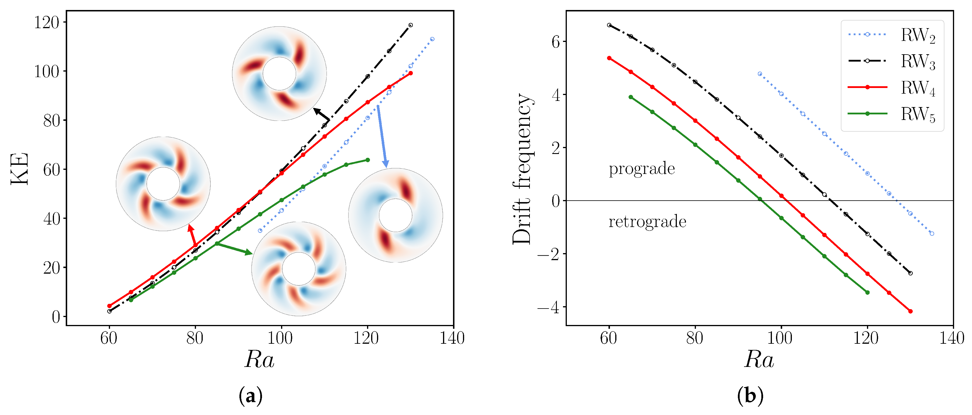
Figure 3.
Velocity fields of rotating waves as the Ekman number is reduced. Shown are: for and ; for and ; for and ; and for and . All of these states have an approximate kinetic energy density of 25. For each field, the radial velocity on the equatorial plane (top) and the azimuthal velocity on a meridional plane (bottom) are shown. As decreases, the convective region becomes more confined to the region of the inner sphere and the flow becomes almost axially independent, according to the Taylor-Proudman theorem. The resolutions used for these simulations were: for at and ; for ; and for .
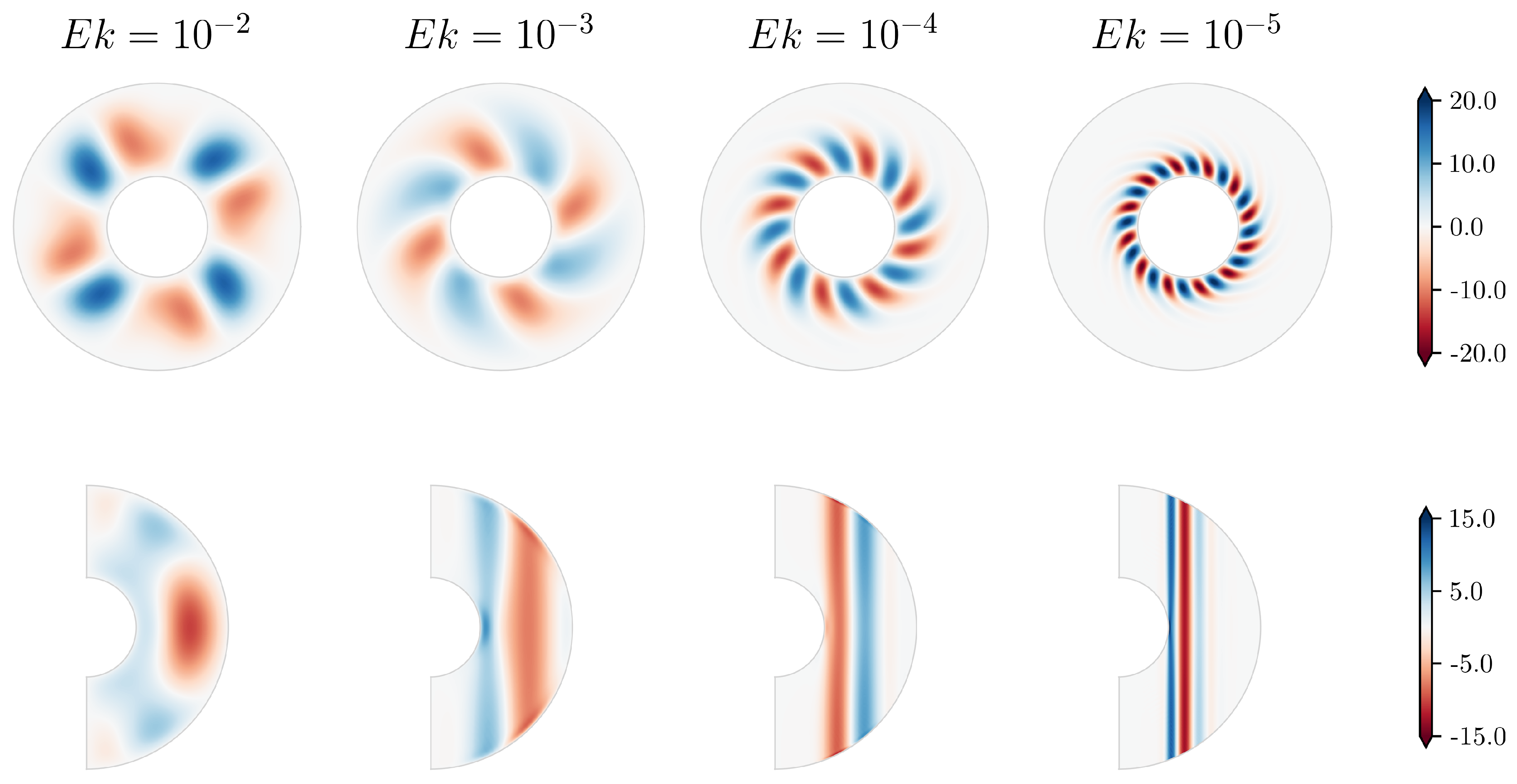
Figure 4.
Flow visualizations for a at and are shown. Top, left to right: , and in the equatorial plane. Bottom, left to right: , and in a meridional plane. The resolution used for this simulation was .
Figure 4.
Flow visualizations for a at and are shown. Top, left to right: , and in the equatorial plane. Bottom, left to right: , and in a meridional plane. The resolution used for this simulation was .
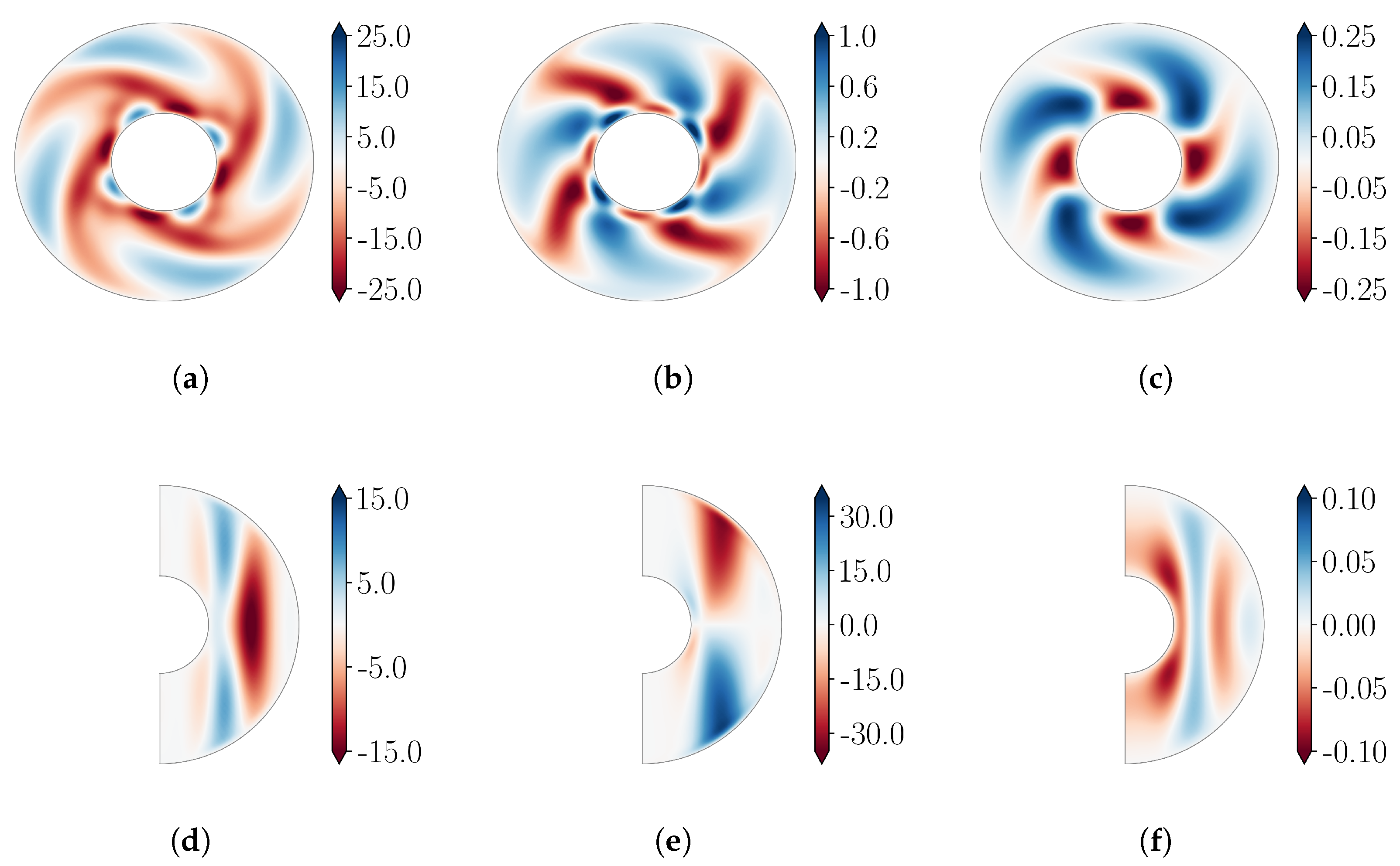
Figure 5.
(a) Block-diagonal matrix. (b) Block-pentadiagonal matrix.
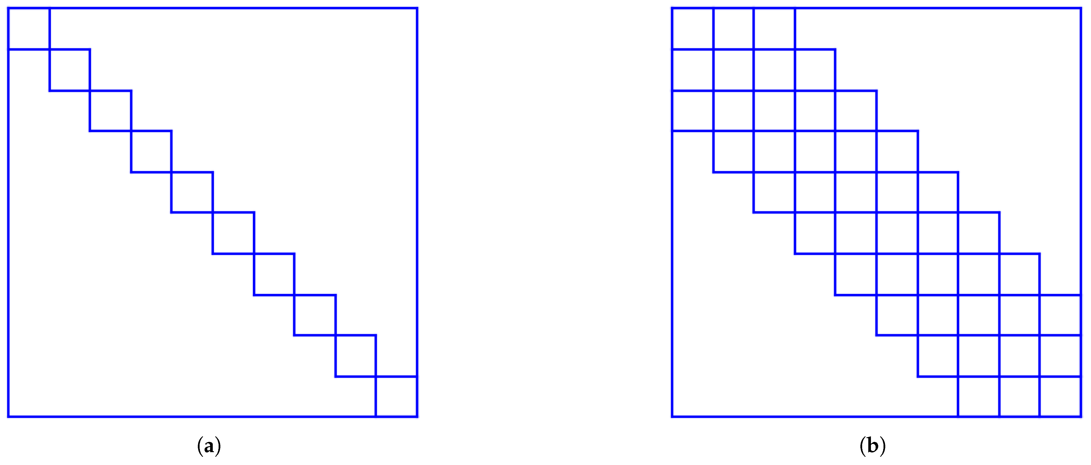
Figure 6.
Bifurcation diagram of rotating wave for as a function of . (a) Kinetic energy. The branch contains three smooth regions separated by two short intervals (at and ) of rapid change containing saddle-node bifurcations. (b) Drift frequency. Three long intervals of almost constant drift frequency are separated by two short intervals of rapid change. The resolution used for this computation was .
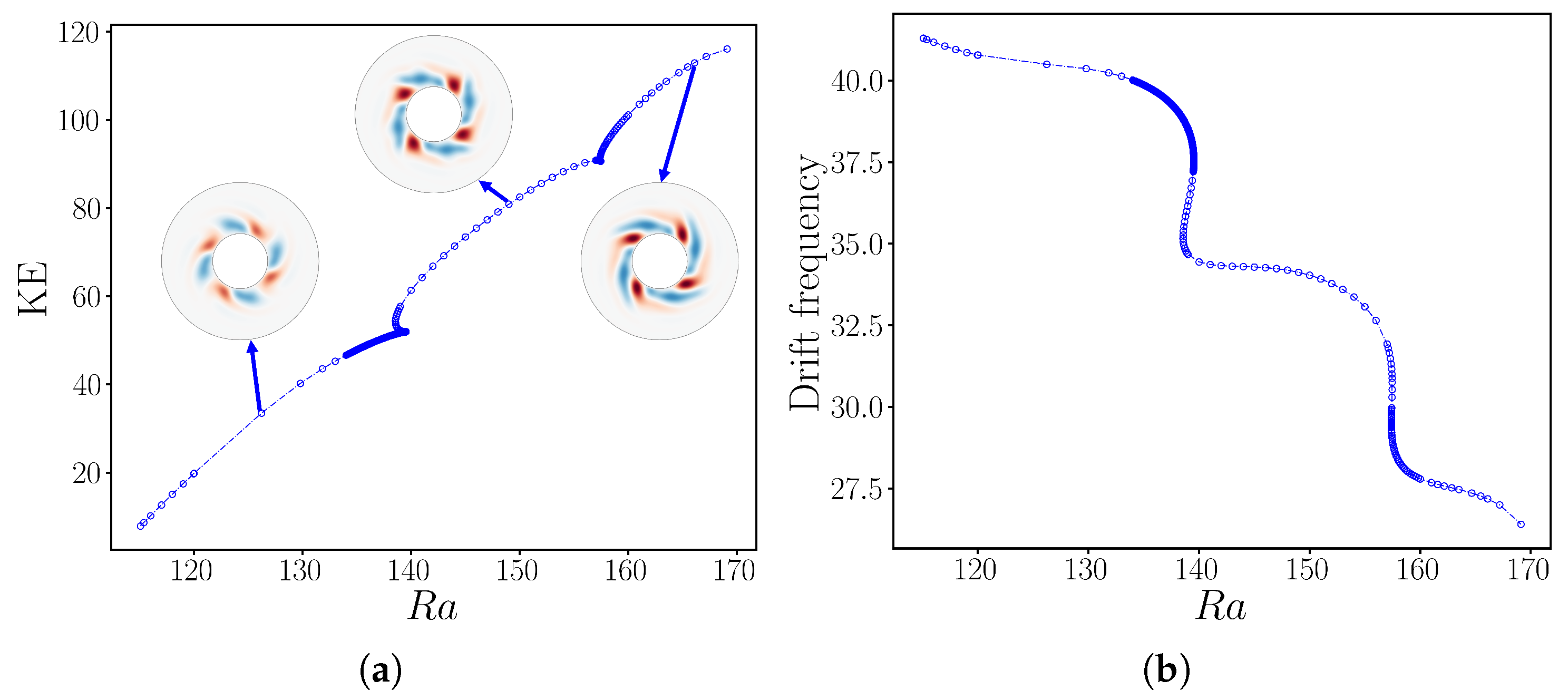
Figure 7.
Bifurcation diagram of rotating wave for as a function of . (a) Kinetic energy. (b) Drift frequency. The branch contains a single interval of rapid change at . The resolution used for this computation was .
Figure 7.
Bifurcation diagram of rotating wave for as a function of . (a) Kinetic energy. (b) Drift frequency. The branch contains a single interval of rapid change at . The resolution used for this computation was .
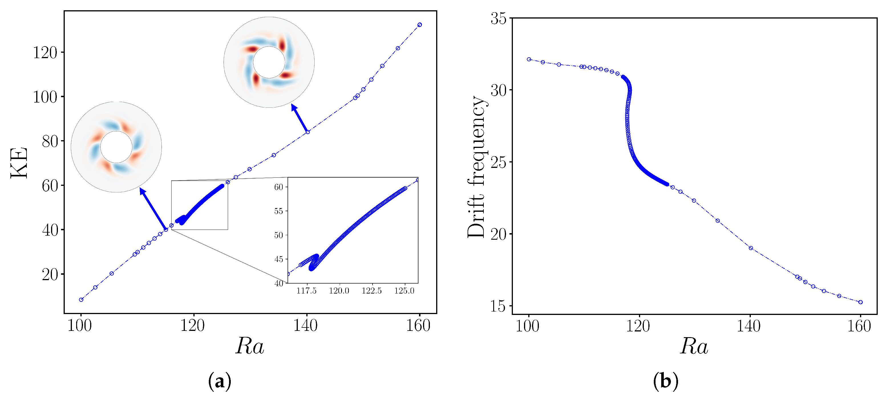
Figure 8.
Bifurcation diagram of rotating wave for as a function of . (a) Kinetic energy. (b) Drift frequency. The branch contains a single interval of rapid change at . The resolution used for this computation was .
Figure 8.
Bifurcation diagram of rotating wave for as a function of . (a) Kinetic energy. (b) Drift frequency. The branch contains a single interval of rapid change at . The resolution used for this computation was .
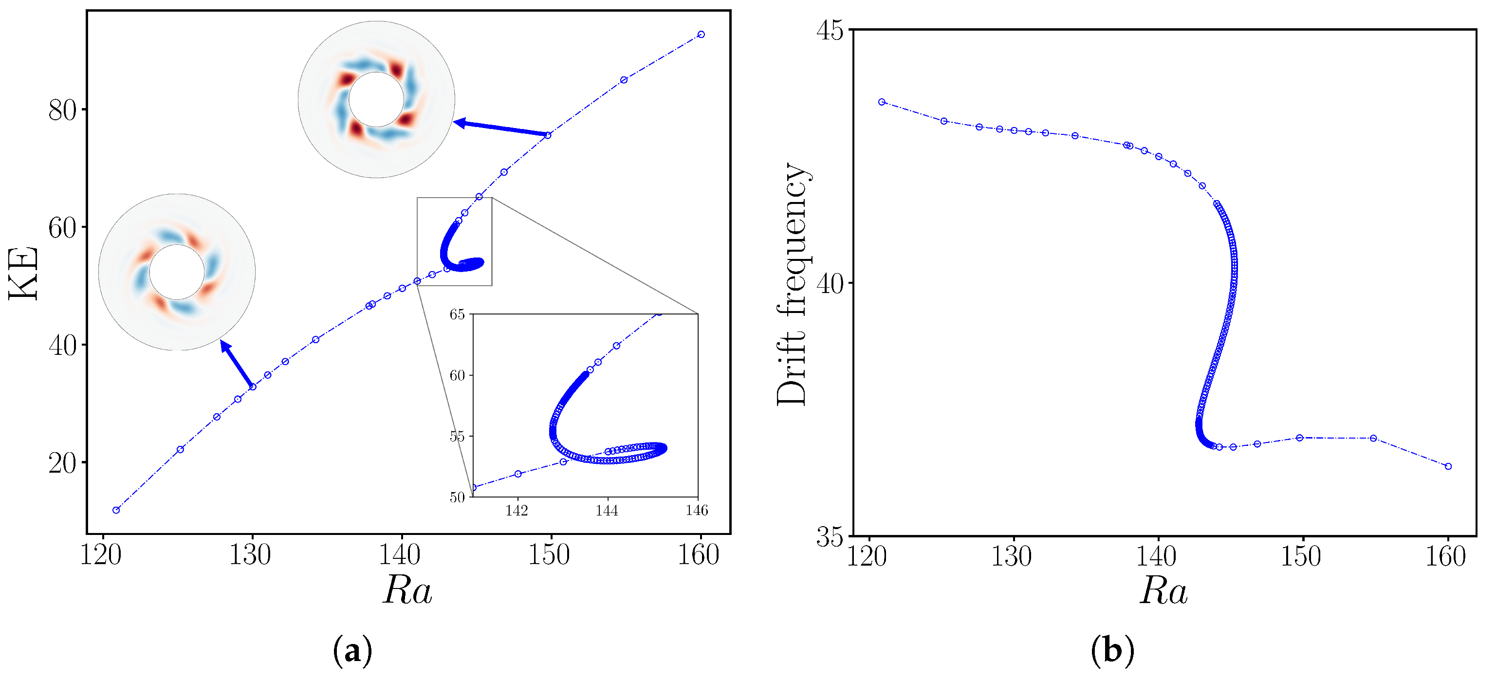
Figure 9.
Bifurcation diagram of rotating wave for as a function of . (a) Kinetic energy. (b) Drift frequency. The branch contains a single interval of rapid change at . The resolution used for this computation was .
Figure 9.
Bifurcation diagram of rotating wave for as a function of . (a) Kinetic energy. (b) Drift frequency. The branch contains a single interval of rapid change at . The resolution used for this computation was .
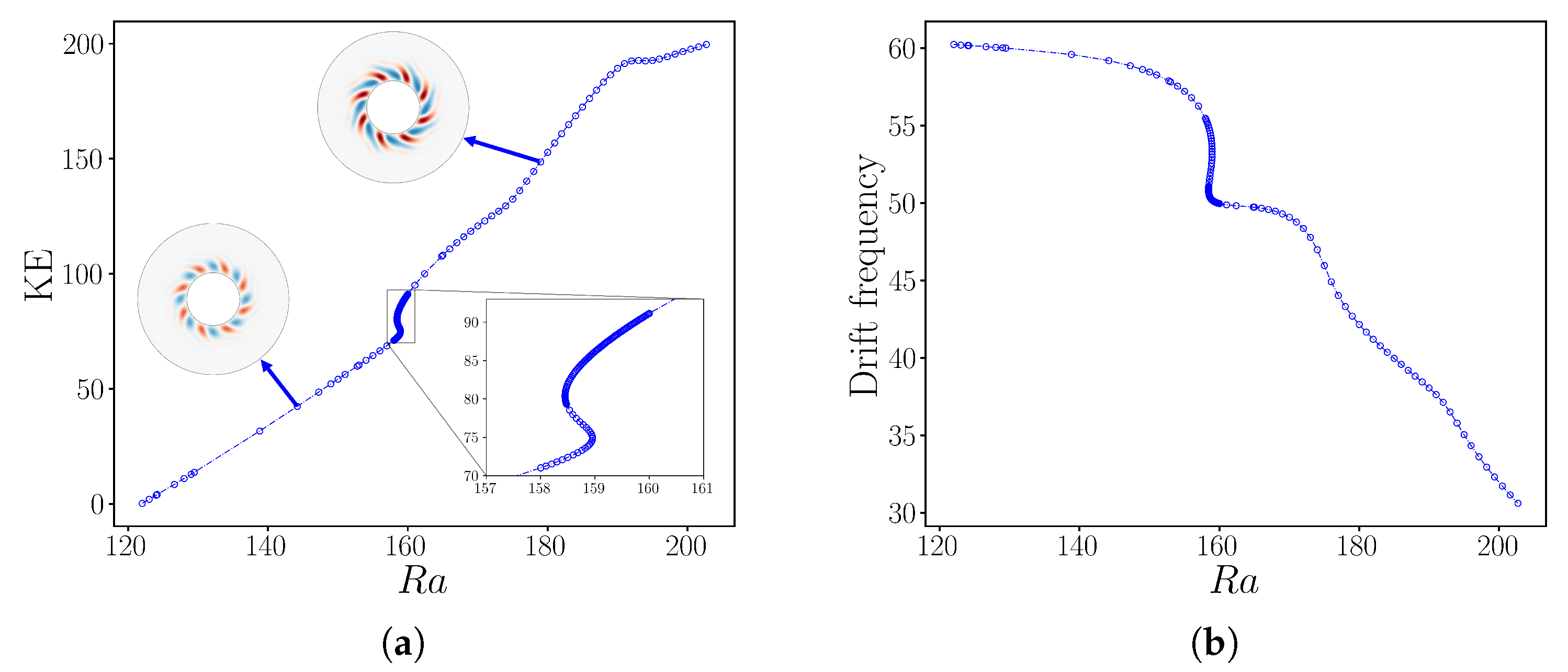
Figure 10.
Bifurcation diagram of rotating wave as a function of , while fixing . (a) Kinetic energy. (b) Drift frequency. Three solution branches exist over the range . The resolutions used for this computation ranged from to .
Figure 10.
Bifurcation diagram of rotating wave as a function of , while fixing . (a) Kinetic energy. (b) Drift frequency. Three solution branches exist over the range . The resolutions used for this computation ranged from to .
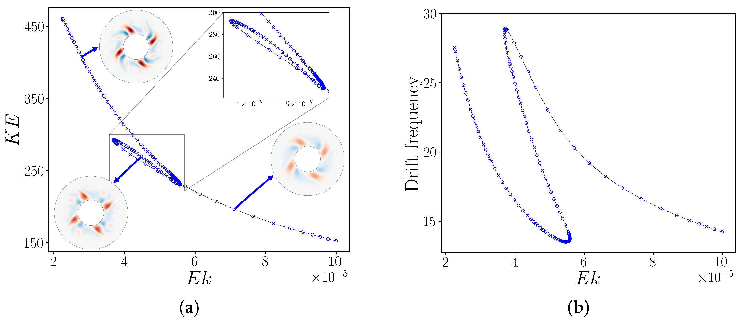
Figure 11.
Total number of matrix-vector actions required by nested Newton-GMRES algorithm to compute as a function of with explicit (dashed) and implicit (solid) implementation of Coriolis force. An average is taken over a branch of values. The number of actions required by the explicit algorithm is always greater than that required by the implicit algorithm, with the ratio between them increasing from approximately 2 at to approximately 9 at . Using the full domain (green) instead of the reduced domain (red) increases the number of GMRES iterations, as well as the cost of each iteration. In average, the full domain requires 1.5 times more actions than the reduced domain counterpart. The explicit algorithm is unsuccessful for . The resolutions used in this case were for the full circle computations and from to for the quarter circle ones.
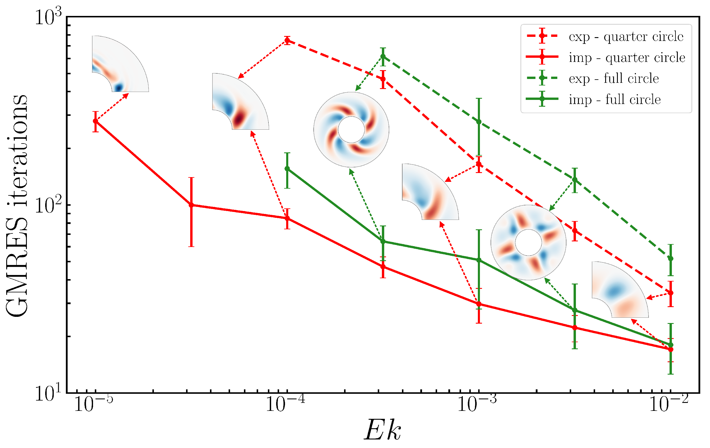
Figure 12.
Total number of matrix-vector actions required by nested Newton-GMRES algorithm to compute (red) and (blue) as a function of with explicit (dashed) and implicit (solid) implementation of Coriolis force.For clarity, the insets show the full domain, although the computations are carried out in reduced domains . An average is taken over many values of . The implicit algorithm is always faster than the explicit algorithm, with the ratio between them of GMRES iterations required increasing from 4 at to 15 at , below which the explicit algorithm fails. The resolutions used for the computations ranged from to .
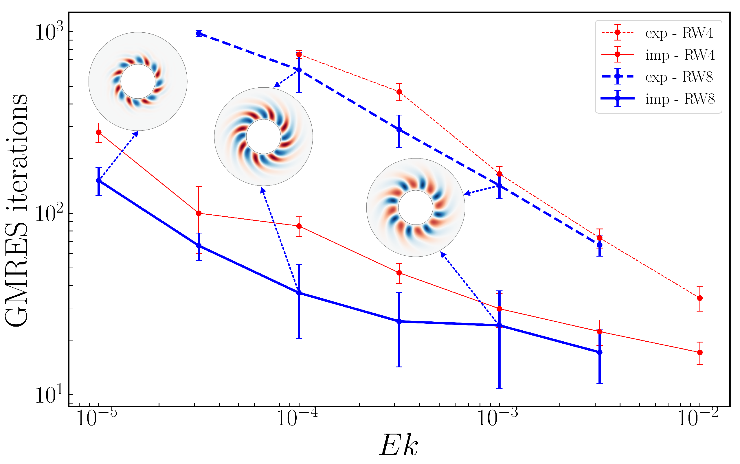
Figure 13.
Total number of matrix-vector actions required by nested Newton-GMRES algorithm to compute (black) and (blue) as a function of with explicit (dashed) and implicit (solid) implementation of Coriolis force. For clarity, the insets show the full domain, although the computations are carried out in reduced domains . An average is taken over a branch of values. The implicit algorithm is always faster than the explicit algorithm for , increasing from a factor of 2.5 for to 20 for , below which the explicit algorithm fails. The resolutions used for the computations ranged from to .
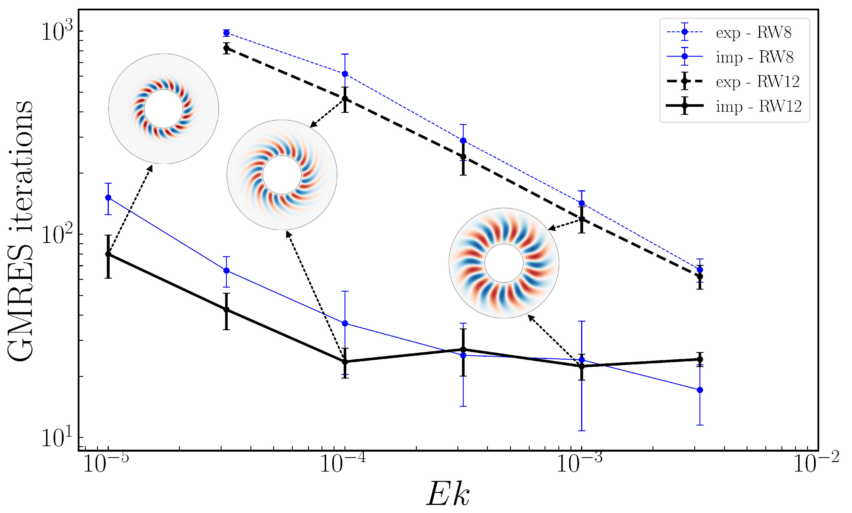
Figure 14.
Accuracy of time-dependent calculation of rotating waves as a function of timestep using implicit (circles) and explicit (crosses) time-stepping of the Coriolis term. Shown is the relative error of the drift velocity as a function of the timestep for various sets of parameter values (see table) where is calculated via Newton’s method. Both the explicit and implicit methods are second order in time, with . Vertical lines indicate the limiting above which explicit time-stepping diverges and cannot be used. The horizontal dashed line indicates . The arrows designate the range of for which implicit timestepping is advantageous: it does not diverge and remains less than . For and , integration using beyond the last point plotted yields qualitatively incorrect states. See also Table 1
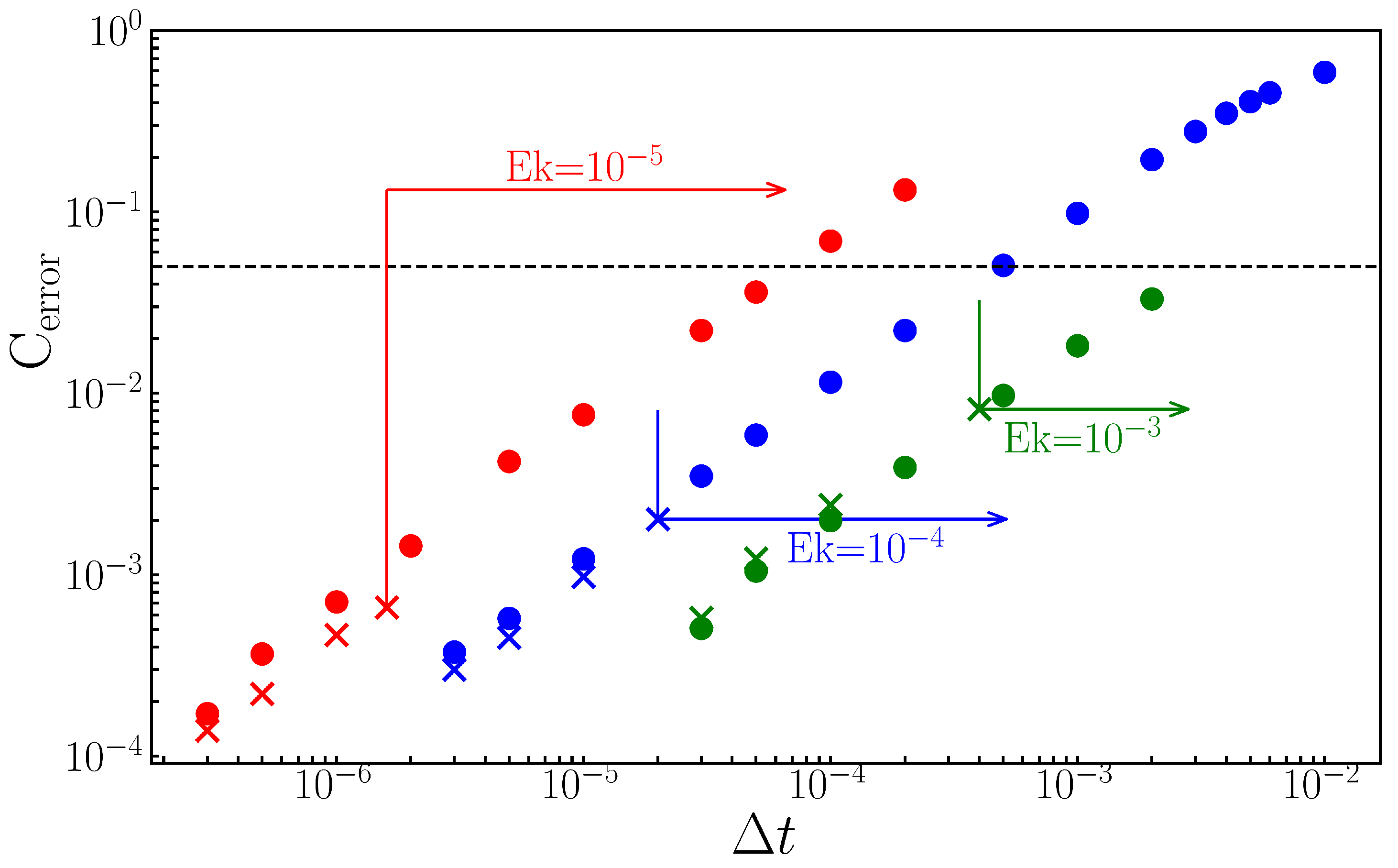

Table 1.
Parameters used for testing and useful range of for implicit time-stepping
| M | explicit diverges | 5% error | ratio | ||||
| 120 | 4 | 70 | |||||
| 130 | 8 | 255 | |||||
| 140 | 12 | 406 |
Disclaimer/Publisher’s Note: The statements, opinions and data contained in all publications are solely those of the individual author(s) and contributor(s) and not of MDPI and/or the editor(s). MDPI and/or the editor(s) disclaim responsibility for any injury to people or property resulting from any ideas, methods, instructions or products referred to in the content. |
© 2025 by the authors. Licensee MDPI, Basel, Switzerland. This article is an open access article distributed under the terms and conditions of the Creative Commons Attribution (CC BY) license (http://creativecommons.org/licenses/by/4.0/).
Copyright: This open access article is published under a Creative Commons CC BY 4.0 license, which permit the free download, distribution, and reuse, provided that the author and preprint are cited in any reuse.


