Submitted:
28 March 2025
Posted:
01 April 2025
You are already at the latest version
Abstract
Corporation’s financial health deterioration may imply financial distress and fraud. Nevertheless, it is computationally intensive to signal financial deterioration earlier since new financial data are periodically available, and these data may outdate an old identification. This study integrates a Naive Bayes classifier with the Bayesian measure of surprise to improve conventional machine learning-based anomaly identification techniques. The latter denotes the anomaly measure, whereas the former classifies past financial ratio data to create a classification model. Defining our anomaly measure employs the relative posterior predictive surprise. For seamless integration with the Naive Bayes classifier’s workflows and pipelines, computing our anomaly measure is a post-processing step in implementing it. Our identified targets are those corporations with declining earnings per share. Experiments on actual financial data show that the Bayesian measure of surprise complements a Naive Bayes classifier in detecting assumed anomalies without labeling past normal or anomalous data and calibrating many parameters. However, our anomaly measure helps signal identified targets earlier than the p-value does. In conclusion, this study has developed a better machine learning-based anomaly detection tool.
Keywords:
corporation’s financial health deterioration
; Bayesian measure of surprise
; Naive Bayes 15 classifier
; anomaly identification
1. Introduction
Emerging information technologies facilitate the continuous and simultaneous monitoring of multiple companies’ financial health. Relying on an auditor to signal financial health deterioration is limited and subjective. Auditors can only check a limited amount of financial data to identify a case of corporation’s financial health deterioration at one time. Their judgments may be subjective and inconsistent. It is computationally intensive to warn of financial health deterioration since we periodically observe new financial data. The latest financial data may outdate an old identification.
This study integrates a Naive Bayes classifier with the Bayesian measure of surprise (e.g., [1]) to improve conventional machine learning-based anomaly identification techniques. The former classifies past financial ratio data to create a classification model, whereas the latter is the anomaly measure. The relative posterior predictive surprise is employed to define our anomaly measure. Our detection targets are those cases with declining earnings per share (EPS).
Creating this study considers the challenges of implementing a machine learning algorithm for anomaly detection. Those challenges are
- Labeled normal or anomalous data may be unavailable. Many machine learning algorithms (e.g., [2]) need to label past normal or anomalous data for detecting future anomalies.
- Reconstructing the past data distributions to detect future anomalies is inconvenient. Models like autoencoders (e.g., [5]) or principal component analyses (e.g., [6]) reconstruct the distribution of past data in detecting unseen anomalies. Implementing this reconstruction is inconvenient when detecting anomalies from periodically updated data.
Choosing the Naive Bayes classifier for this study focuses on its performance in classifying high-dimensional datasets. Compared to other classification algorithms, such as the random forest classifier and support vector machines model, a Naive Bayes classifier classifies high-dimensional data fast and outputs the good classification accuracy (e.g., [7]). Besides, a Naive Bayes classifier outputs posterior probabilities. These outputs facilitate the computation of relative posterior predictive surprise (e.g., [1]) to define the Bayesian measure of surprise. Thus, it is possible to seamlessly integrate this Bayesian measure of surprise with machine learning workflows and pipelines.
Selecting the Bayesian measure of surprise considers the detection of an anomaly without labeling normal or anomalous data. We have reviewed published expressions of the Bayesian measure of surprise [8]. Defining these expressions can use the marginal likelihood. They meet the requirement of detecting anomalous financial health without labeling normal and abnormal data.
This study intends to provide the following contributions:
- Balance some advantages of applying unsupervised, semi-supervised, and supervised learning approaches [9] to anomaly detection. We adapt future anomalies without labeling past financial data. Adapting new anomalies and eliminating the need for labeling data are two of the advantages of unsupervised anomaly detection. Meanwhile, this study defines a Bayesian measure of surprise to signal anomalies. This Bayesian measure of surprise is explainable and interpretable. Explainability and interpretability are two of the advantages of creating a supervised anomaly detection. Besides, we detect financial health deterioration without calibrating many nuisance parameters. Eliminating the need for this calibration is one of the advantages of generating semi-supervised anomaly detection.
- This study does not preprocess past high-dimensional financial data before detecting new anomalies based on these data. We further implement the computation of a Bayesian measure of surprise using classification results of a Naive Bayes classifier. Except for high-dimensional financial data, the current works may be suitable for detecting anomalies from other high-dimensional data.
- This study seamlessly integrates a classification algorithm with an anomaly measure. Computing the Bayesian measure of surprise is a post-processing step of implementing a Naive Bayes classifier. It is unnecessary to create new codes to implement a Naive Bayes classifier and the Bayesian measure of surprise.
The remainder of this study has five sections. Section 2 reviews the published research relevant to this study. Section 3 presents a Naive Bayes classifier and our Bayesian measure of surprise. We present the application of the resulting works in this section to three experiments in Section 4. Section 5 presents the discussions based on the results of Section 4. Section 6 presents the conclusions of this study.
2. Literature Review
Before creating this study, we reviewed some published articles that describe machine learning-based anomaly detection techniques. A quick review of these articles finds that we categorize them into supervised, semi-supervised, and unsupervised learning approaches [9]. A supervised learning approach means that we labeled past normal and anomalous data before anomaly detection, whereas an unsupervised learning approach does not need labeled data. A semi-supervised learning approach employs only labeled normal data.
We have three concerns after reviewing different anomaly detection methods:
- Advantages and disadvantages of those supervised, semi-supervised, and unsupervised learning approaches;
- Strengths and weakness of a machine learning-based anomaly detection technique;
- Drawbacks of a likelihood-based anomaly measure.
2.1. Advantages and Disadvantages of Supervised, Semi-Supervised, and Unsupervised Learning Approaches
Choosing a supervised learning approach to detect anomalies requires labeled normal and anomalous data. Requiring labeled data is one of the disadvantages of a supervised learning approach [10]. Therefore, some researchers developed semi-supervised or other methods (e.g., [10]) for employing less labeled data. However, labeling normal and abnormal data results in the accurate detection of anomalies. It is one of the advantages of supervised anomaly detection. However, the accurate detection may cause another risk of overfitting (e.g., [11])
In contrast, unsupervised anomaly detection has the advantage of needing no labeled data [12]. However, the corresponding disadvantage is higher false positive rates. An unsupervised learning approach may alert too many false anomalies (e.g., [12]). Meanwhile, some previous studies have concluded that unsupervised anomaly detection can adapt unseen anomalies (e.g., [10]). Nevertheless, attaining this adaptability may require the continuous calibration of many parameters (e.g., [14]). Completing the calibration is computationally intensive when new data are periodically available.
Compared to the development of supervised and unsupervised learning approaches, developing a semi-supervised learning approach creates universal measures for labeling limited normal data. For example, Lee et al. [15] design a probabilistic anomaly measure for identifying new anomalies. Defining this probabilistic anomaly measure used the densities of limited normal data. However, we can quickly expect that they must collect sufficient normal data to generate accurate probabilistic anomaly measures. Nico et al. [10] defined a loss function for detecting a new anomaly. This loss function describes the distance of a point to the center of a class on the hyperplane generated by a support vector machines model. Gao et al. [16] used the DBSCAN method to cluster the normal data and defined the Euclidean distance for determining whether a new data instance is anomalous.
2.2. Strengths and Weakness of a Machine Learning-Based Anomaly Detection Technique
A published article [9] reviewed the applications of machine learning algorithms to anomaly detection. The strengths of these applications include filtering out rare anomalies, eliminating the need for labeling data, adaptability to various domains, real-time processing, handling streaming, high-dimensional, or large datasets (e.g., [9]). However, these strengths do not affect this study.
The weakness of a machine learning algorithm in anomaly detection alerts this study. For example, Zhang et al. [17] found that anomaly detection using a machine learning algorithm encountered the difficulty of detecting rare and diversely distributed anomalies. Therefore, they formulated a new approach to overcome this weakness. Nevertheless, implementing this previous study still used labeled data. Khloud et al. [18] noticed the high false-positive rates output by a machine learning-based anomaly detection; therefore, they developed a deep learning model to reduce false-positive rates.
Nevertheless, we can expect that it is difficult to interpret and finely tune the resulting deep-learning model. Razzak et al. [19] improved the cure of dimensionality and overfitting in applying the conventional one-class tensor machine to large-scale anomaly detection with high-dimensional and noisy data. This cure of dimensionality refers to various phenomena that arise when analyzing data in high-dimensional spaces that do not occur in low-dimensional settings. Another apparent weakness is the metrics for indicating what is normal or anomalous. Published studies (e.g., [18,19]) had no choice but to use metrics such as F1 score and precision to judge whether anomalies are successfully detected. These metrics were employed to measure the classification accuracy.
2.3. Drawbacks of a Likelihood-Based Anomaly Measure
If one reviews existing anomaly measures, one may find that a specific machine learning algorithm must incorporate the right anomaly measure in detecting anomalies. For example, if we construct a support vector machines model [19] for anomaly detection, we prefer a distance-based anomaly measure.
Since this study defines the Bayesian measure of surprise based on the relative posterior predictive surprise, we are interested in the existing drawbacks of a likelihood-based anomaly measure but not interested in the comparison of likelihood-based and other types of anomaly measures. Existing drawbacks relevant to this study are
- Published studies (e.g., [19]) assume that normal data follows a particular probability distribution. Therefore, we can detect anomalies by checking whether suspicious data conform unacceptably to that particular probability distribution. Unfortunately, this assumption does not hold in practice, especially with complex real-world data.
- Some machine learning models (e.g., [16]) (e.g., a deep learning model) are complex. Obtaining their best performance requires tuning many parameters. We need ablation studies to determine the best values of these parameters.
- A likelihood-based anomaly measure may miss anomalies that only deviate from expected behavior within a certain context or subspace (e.g., [20]).
- Likelihood-based anomaly measures may be sensitive to noisy data. Noisy data may be misclassified as anomalies (e.g., [21]).
- Calculating likelihood-based measures for relatively high-dimensional data may be challenging and computationally expensive (e.g., [19]).
The drawbacks mentioned above are necessary cautions in implementing this study.
3. Methods
3.1. Naive Bayes Classifier
This study chooses a Naive Bayes classifier (e.g., [22]) to classify past financial data. A Naive Bayes classifier classifies data according to their posterior probabilities. We can employ posterior probabilities to define Bayesian measures of surprise [23].
Suppose we have collected historical financial ratios of N companies to create a classification model and these financial ratios are group into where , and is the j-th financial ratio of and n is the total number of chosen financial ratios. For classifying those data, represent reserved class variables. Besides, we may continuously observe new financial ratio data to update the .
A Naive Bayes classifier is a supervised multi-class classification algorithm. As shown in Figure 1, building a Naive Bayes classifier considers Bayes’ theorem with conditional independence assumption between every pair of variables:
in which , is the posterior probability, denotes the likelihood, and is the prior probability.
Applying the assumption that financial ratios are conditionally independent of each other yields
where . Since the denominator of Equation (2) is the same for all classes, comparing the numerator of it for each class is implemented in classifying , . This comparison ends when Equations (3)-(4) are satisfied:
where denotes a class variable.
3.2. Bayesian Measure of Surprise
Suppose denotes a null hypothesis for describing the financial health of N companies. For example, this null hypothesis may assume that the data vary according to a specific probability distribution. If we classify the data, this is a member of a class. As time progresses, the updates the .
Once the updates the , whether the still satisfies the null hypothesis is questioned. Therefore, we define and calculate the Bayesian measure of surprise as a quantitative answer to this question. If the resulting Bayesian measure of surprise is significantly lower, the is surprising or anomalous. However, one may not be confident in determining whether the null hypothesis is rejected; therefore, we introduce a significance level to quantify the confidence.
Statistics say that rejecting the null hypothesis can use the p-value. If the resulting p-value is less than a specific significance level , one rejects the null hypothesis and the corresponding is anomalous or surprising: (e.g., [24])
in which f denotes a probability density function. The lower the p-value, the more anomalous or surprising the . Furthermore, Good (1956) [25] concluded that calculating the relative predictive surprise R can provide a more accurate quantitative measure for rejecting the null hypothesis. Thus
in which is the supermum. However, constructing an exact probability density function f may be difficult. For example, new data may be frequently available. Therefore, continuously updating the exact probability density function f may be necessary. This updating is not beneficial for the short-time processing. A possible way to avoid such a step is to fit collected data into an approximated probability density function. Thus, Equations (5)-(6) are modified to compute the plug-in Bayesian measure of surprise and relative predictive surprise :
where ^ indicates the approximation. Moreover, we may eliminate the necessity of building an approximated probability density function by computing the marginal likelihood ([8]) and modify Equation (7) to
in which is the prior predictive p-value and is the relative prior predictive surprise. Nevertheless, once the updates the , the probability distribution of those data changes. Therefore, we apply the Bayes’ theorem to re-calculate the marginal likelihood by within the class and modify Equation (8) to ([23])
where is the posterior p-value and is our relative posterior predictive surprise.
4. Results
This study introduces actual financial ratio data generated by listed companies in Taiwan’s stock market to test Equations (3)-(4), the , and . The TEJ database (http://schplus.tej.com.tw) is our data source.
4.1. Experiment 1
Referring to a previous article [26], we download data on the EPS, debt ratio, return on assets (ROA), and total asset turnover in the fourth quarter of 2023 to build a classification model. Figure 2 visualizes the ranges of EPS, debt ratio, ROA, and asset turnover ratio values. The total number of data N is 1958.
A higher EPS value can suggest that a company shows strong profitability and efficient use of capital. Instead, a lower EPS value can indicate operational inefficiencies, excessive investment in non-performing assets, or competitive pressures. The company is creating less profit per share. A higher debt ratio can indicate such as increased financial risks and potential bankruptcy. If a company keeps moderate debts, it has a valuable tool for financing growth initiatives, such as expansion or research and development. A higher ROA value can signal that a company is effectively employing its assets to generate profits, whereas consistently low ROA values may signal financial health deterioration. It implies that a company is not efficiently utilizing its assets to generate profits. The total asset turnover quantifies the ability to employ a company’s assets to create revenue effectively. A low total asset turnover may imply poor inventory management, underutilized equipment, or inefficient processes.
We create a classification model according to the following class variable :
in which this study assumes that each class contains companies with similar financial health. If a company’s EPS is above 10, we assume that its financial health is strong.
Meanwhile, we use 25% of the data as the test data, whereas the rest is the train data. As performance benchmarks, we choose a logistic regression model and a neural network as two baseline models. The AUC (Area under the ROC curve) is the main metric for quantifying the classification accuracy. Constructing the neural network employs two hidden layers and equips each hidden layer with four neurons. Setting other necessary hyperparameters adopts defaults of Python’s scikit-learn package.
Figure 3 compares the resulting ROC curves in which NB, LR, and NN are abbreviations of the Naive Bayes classifier, logistic regression, and neural network, respectively. Equations (3)-(4) output the confusion matrix in Figure 3. We use this confusion matrix to compute other metrics to describe classification accuracy. Table 1 lists these metrics.
Observing Figure 3 can find that Equations (3)-(4) outperform the other two classification algorithms in classifying financial data in this example. The resulting AUC values are 0.988 (Naive Bayes classifier), 0.977 (logistic regression), and 0.975 (neural network). The resulting AUC values indicate that all three classification algorithms provide sufficiently accurate classification models; however, Equations (3)-(4) outperform the other two classification algorithms.
Next, this study calculates the and to identify those companies subjected to declining EPS values. In other words, we preliminarily choose such companies as identification targets. A declining EPS value may indicate such as decreasing revenues and inefficient management. It may be as an early signal of financial health deterioration. EPS, debt ratio, ROA, and total asset turnover data in the first quarter of 2024 are further downloaded. After inspecting these new financial data, total 1449 listed companies are our identification targets. Their EPS values declined between the fourth quarter of 2023 and first quarter of 2024. The previous criterion and [1] are the rules for judging the successful or unsuccessful identifications of a target.
Figure 4(a)-Figure 4(d) illustrate the identification results. Black points in Figure 4 denote those 1449 identification targets. A red point in Figure 4(a)-Figure 4(d) denotes the successful identification of a target using the or , whereas a blue point in the same figures represents the successful identification of a target using only the .
Inspecting blue and red points in Figure 4(a)-Figure 4(d) finds that calculating the can signal declining EPS values earlier than computing the does. These four figures indicate that some blue points are close to the gray 45-degree line. These blue points represent that the chosen financial ratios changed slightly between the fourth quarter of 2023 and the first quarter of 2024. An example is the Globe Industries Co. (Stock No = 1324). It had EPS = 0.53, debt ratio = 19.85, ROA = 2.72, and total asset turnover = 0.77 in the fourth quarter of 2023. These financial ratios changed to EPS = 0, debt ratio = 19.26, ROA = 0.35, and total asset turnover = 0.66 in the first quarter of 2024. Consequently, Globe Industries Co. was less profitable and less efficient in utilizing its resources. Meanwhile, an example of red points is the RichWave Tech. Co. (Stock No = 8066). It provided EPS = 0.74, debt ratio = 57.75, ROA = 2.71, and total asset turnover = 3.15 in the fourth quarter of 2023. These financial ratios were EPS = 0.16, debt ratio = 50.98, ROA = 2.69, and total asset turnover = 2.9 in the first quarter of 2024. Compared to the Globe Industries Co., these EPS and ROA values changed more apparently.
Meanwhile, counting the total number of blue and red points finds that calculating the identifies 9 % more targets than computing the does. This 9 % is calculated by the expression
However, Figure 4(a)-Figure 4(d) also show unsuccessful identification of some targets. After inspecting the original data, this study categorized these failed targets into two types:
- A company’s financial health remained sufficiently strong between the fourth quarter of 2023 and the first quarter of 2024. An example is the EST Global Apparel Co. Ltd. (Stock No = 4413). Its financial ratios are EPS = 62.52, debt ratio = 13.97, ROA = 58.42, and total and asset turnover = 1.27 in the fourth quarter of 2023. In contrast, these financial ratios changed to EPS = 24.48, debt ratio = 9.72, ROA = 17.76, and total asset turnover = 1.11 in the first quarter of 2024. This company’s financial health kept sufficiently strong.
- The financial health of the company deviated slightly between the fourth quarter of 2023 and the first quarter of 2024. Our classification results indicate that this company’s past and new financial ratio data are in the same class. An example is TBI Motion Technology Co. Ltd. (Stock No = 4540). Its financial ratios in the fourth quarter of 2023 are EPS = -1.09, debt ratio = 58, ROA = -1.34, and total asset turnover = 0.33, whereas these financial ratios changed to EPS = -1.71, debt ratio = 58.73, ROA = -2.15, and total asset turnover = 0.31 in the first quarter of 2024.
4.2. Experiment 2
Describing the financial health of a company may use different groups of financial ratios. In the second experiment, we change to use the EPS, debt ratio, ROE, and dividend yield in the third quarter of 2023 to construct another classification model. Figure 5 shows the ranges of these financial ratio data. The total number of data N is 1952.
The ROE is a financial metric measuring a company’s probability in relation to shareholders’ equity. A higher ROE can suggest that a company is efficient at creating profits using every unit of shareholders’ equity. Meanwhile, a high dividend yield may indicate that a company is in financial health deterioration. This company’s shares may have fallen in response to financial troubles. It has not cut its dividend yet.
We still classify financial data according to Equation (11), Besides, we employ 25% of the data as the test data, whereas the rest is the train data. Figure 6 shows the resulting ROC curves. Equations (3)-(4) output the confusion matrix shown inside Figure 6.
From the confusion matrix inside Figure 6, we calculate Table 2. Besides, calculating the AUC values from Figure 6 yields 0.994 (Naive Bayes classifier), 0.98 (logistic regression), and 0.983 (neural network). These results and Table 2 support that all three classification algorithms can provide sufficiently accurate classification models for the current experiment.
Like Section 4.1, this study preliminarily selects those companies subjected to declining EPS values as identification targets. Therefore, we download EPS, ROE, debt ratio, and dividend yield data measured in the fourth quarter of 2023. These new financial data indicate that 626 companies are our identification targets. The criteria and are still the rules for determining the successful or unsuccessful identification of targets. Figure 7(a)-Figure 7(d) show the identification results.
Comparing red and blue points in Figure 7(a)-Figure 7(c) finds that most of the blue points are close to the 45-degree line. Similar to Section 4.1, this comparison may imply that computing signals the financial health deterioration earlier. Meanwhile, Figure 7(d) may indicate that the dividend yield is less suitable for alerting financial health deterioration. Blue and red points do not hide most of the black points.
An example of blue points in Figure 7(a)-Figure 7(d) is the Tainergy Technology Co. Ltd. (Stock No = 4934). Its financial ratios are EPS = 0.94, ROE = 4.72, debt ratio = 20.87, and dividend yield = 0 in the third quarter of 2023. These financial ratios changed to EPS = -0.13, ROE = -9.28, debt ratio = 24.61, and dividend yield = 24.61 in the fourth quarter of 2023. They indicate that Tainergy Technology Co. Ltd. is less profitable and signals financial strains. Meanwhile, an example of red points is Mercuries Life Insurance Inc. (Stock No = 2867). Its financial ratios were EPS = -0.46, ROE = 20.45, debt ratio = 97.52, and dividend yield = 0 in the third quarter of 2023. These financial ratios changed to EPS = -2.11, ROE = 17.56, debt ratio = 97.38, and dividend yield = 97.38 in the fourth quarter of 2023. The EPS and ROE values remained poor, but the dividend yield rose apparently. The rising dividend yield can result from a declining stock price, which might indicate financial struggles.
Meanwhile, counting the total number of blue and red points finds that calculating the identifies 20 % more targets than computing the does.
Nevertheless, Figure 7(a)-Figure 7(d) also show unsuccessful identification of some targets. After inspecting the original data, we categorize such failed targets into two types. Thus
- Similar to Section 4.1, the current section fails to identification targets whose financial health remained sufficiently strong or poor between third and fourth quarters of 2023. An example is the Launch Technologies Co. Ltd. (Stock No = 8420). It generated EPS = -12.97, ROE = -53.87, debt ratio = 58.1, and dividend yield = 9.24 in the third quarter of 2023. These financial ratios changed to EPS = -17.4, ROE = -80.86, debt ratio = 66.37, and dividend yield = 0.0 in the fourth quarter of 2023. These financial ratios show that the company’s financial health kept poor.
- Figure 7(a), Figure 7(c), and Figure 7(d) show that many unsuccessful identification of companies subjected to declining EPS values but increasing debt ratios and dividend yields between third and fourth quarters of 2024. Conclusively, the financial health of these companies may not be deteriorating. We need more financial ratios to conclude the financial health deterioration. An example is the GeneReach Biotechnology Co. (Stock No = 4171). It provided EPS = -1.88, ROE = -10.84, debt ratio = 23.54, and dividend yield = 9.43 in the third quarter of 2023, whereas these financial ratios changed to EPS = -2.89, ROE = -17.43, debt ratio = 26.67, and dividend yield = 26.67 in the fourth quarter of 2023.
4.3. Experiment 3
In Figure 4(a) and Figure 7(a), identifying some black points close to the 45-degree line fails. Therefore, we test to create a third experiment with the goal of improving the identification of black points close to the 45-degree line. This experiment employs EPS, operating profits per share, debt ratio, and total asset turnover in the second quarter of 2024 to build a classification model. Figure 8 describes the ranges of these financial ratios. The total number of data N is 2362.
The succeeding experiment changes the class variable to
Different from Equation (11), this study defines Equation (12) by considering that two companies with the difference of their EPS values below 2 have similar financial health in defining the class variables .
Meanwhile, we employ 25% of the data as the test data, whereas the rest is the train data. We use Equations (3)-(4), a logistic regression model, and a neural network to create three classification models. Figure 9 shows the resulting ROC curves. Equations (3)-(4) output a confusion matrix shown inside Figure 9. Based on this confusion matrix, we calculate Table 3. Besides, calculating the AUC values from Figure 9 yields 0.994 (Naive Bayes classifier), 0.962 (logistic regression), and 0.984 (neural network).
Compared to Section 4.1 and Section 4.2, Figure 9 may indicate that we have improved the classification accuracy. Although the chosen financial ratios are different, the resulting AUC values are better in this section. However, those AUC values indicate that the current three classification algorithms provide three sufficiently accurate classification models.
We still choose those companies subjected to declining EPS values as preliminary identification targets. Therefore, EPS, operating profits per share, debt ratio, and total asset turnover values in the third quarter of 2024 are further downloaded. The criteria and are still the rules for determining successful or unsuccessful identifications of targets. Figure 10(a)-Figure 10(d) describe the identification results.
Compared to Section 4.1 and Section 4.2, the succeeding experiment is more successful in identifying companies subjected to declining EPS values (between the second and third quarters of 2024). We see fewer black points in Figure 10. In Figure 10(a), blue points are close to the (0,0) point. They indicate that computing the signals earlier the subtle changes of chosen financial ratios. It can provide an early alert of financial health deterioration. An example of blue points is the TIGA Gaming. Inc. (Stock No = 6536). This company had EPS = 0.51, operating profits per share = 0.47, debt ratio = 47.28, and total asset turnover = 1.26 in the second quarter of 2024. These financial ratios changed to EPS = -0.88, operating profits per share = -1.1, debt ratio = 46.2, and total asset turnover = 0.33 in the second quarter of 2024. We can see that both EPS and operating profits per share reduced between the second and third quarters of 2024. The total asset turnover also declined. As a consequence, the TIGA Gaming. Inc. was less profitable and efficient in utilizing its resources.
Meanwhile, an example of red points is Cheer Time Enterprise Co. Ltd. (Stock No= 3229). This company had EPS = 0.3, operating profits per share = 0.15, debt ratio = 28.99, and total asset turnover = 0.99 in the second quarter of 2024. These financial ratios changed to EPS = 0.11, operating profits per share = 0.02, debt ratio = 27.79, and total asset turnover = 1.01. Compared to the last example, this company’s profits have apparently declined more.
Counting the total number of blue and red points finds that calculating the identifies 5 % more targets than calculating the .
An example of black points in Figure 10(a)-Figure 10(d) is the Formosa Petrochemical Co. (Stock No = 6505). This company had EPS = 0.81, operating profits per share = 0.46, debt ratio = 22.5, and total asset turnover = 1.62 in the second quarter of 2024. These financial ratios changed to EPS = 0.49, operating profits per share = -0.04, debt ratio = 17.99, and total asset turnover = 1.72. It is difficult to say that this company’s financial health deteriorated. The company’s declining EPS and operating profits per share conflict with improved debt ratio and total asset turnover.
5. Discussion
- In identifying companies subjected to declining EPS values, this study does not label normal or anomalous data in Section 4. Instead, we classifies data before detecting such companies.
- In Section 4.1-Section 4.3, the Bayesian measure of surprise is a good early alert of a company’s financial health deterioration. Calculating it identifies 5%-20% more chosen targets than computing the conventional p-value does.
- Since the computation of Equation (10) does not change the original workflow and pipeline of a Naive Bayes classifier, we seamlessly combine Equations (3), (4), and (10). One can modify old codes to implement a Naive Bayes classifier for anomaly identification.
- If we desire to signal anomalies as early as possible, Section 4.3 suggests finely discretizing variation of EPS values to generate a classification model.
- Equation (10) does not contain the reconstruction of input data distributions and calibration of many nuisance hyperparameters.
- Implementing Section 4.1-Section 4.3 uses financial data containing four financial ratios. Computing Equation (10) using these high-dimensional data is not challenging or computationally intensive.
- Tuning the significance level can improve those unsuccessful identifications in Section 4.1-Section 4.3. Nevertheless, too high values may destroy the rarity of identified anomalies.
6. Conclusions and Concluding Remarks
This study integrates a Naive Bayes classifier and the Bayesian measure of surprise to build a new and machine learning-based anomaly identification tool. In Section 4, implementing the resulting tool to study the suspicious financial health deterioration of listed companies in Taiwan’s stock market. We first use the Naive Bayes classifier to construct a classification model of input financial data and next calculate the Bayesian measure of surprise based on classification results. Without reconstructing input data distributions and labeling of normal or abnormal data, the Bayesian measure of surprise helps identify 5%-20% more assumed financial health deterioration than computing the conventional p-value does.
From the results in Section 4, this study concludes:
- A Naive Bayes classifier and the Bayesian measure of surprise can be seamlessly combined as a good machine learning-based anomaly identification tool. The resulting tool helps an auditor identify 5%-20% more suspicious anomalies.
-
Compared to other anomaly measures, the Bayesian measure of surprise has the following advantages:
- Reconstructing the input data distributions is unnecessary.
- Labeling normal and anomalous data is not required.
- Requiring tuning only one parameter.
Furthermore, we recommends to finely discretize variation of financial ratios for capturing subtle changes of financial ratios. Thus, calculating the Bayesian measure of surprise can signal financial health deterioration earlier.
This study has some limitations. Companies of different industries may have different financial performance. Therefore, different significance levels may be set capture their financial health deterioration. Searching ideal values for a specific industry may be the goal of a future research. Besides, recent regulations prevent the real-time computation of our anomaly measure. We can’t obtain the financial data in real-time.
Author Contributions
Conceptualization, G.Y. Sheu; methodology, G.Y. Sheu; software, G.Y. Sheu; validation, G.Y. Sheu; formal analysis, G.Y. Sheu; investigation, G.Y. Sheu; resources, H.Y. Lin; data curation, H.Y. Lin; writing—original draft preparation, G.Y. Sheu; writing—review and editing, G.Y. Sheu; visualization, H.Y. Lin; supervision, G.Y. Sheu; project administration, G.Y. Sheu. All authors have read and agreed to the published version of the manuscript.
Funding
This research received no external funding.
Data Availability Statement
The research data are available at http://schplus.tej.com.tw. They are also available at https://github.com/xsheu/applied_sciences.
Conflicts of Interest
The authors declare no conflicts of interest.
References
- Bayarri, M.J.; Morales, J. Bayesian measures of surprise for outlier detection. J. Stat. Plan. Inference 2003, 111(1-2), 3–22. [Google Scholar] [CrossRef]
- Razzak, I.; Zafar, K.; Imran, M.; Xu, G. Randomized nonlinear one-class support vector machines with bounded loss function to detect of outliers for large scale IoT data. Future Gener. Comp. Sy., 2020, 112, 715–723. [Google Scholar] [CrossRef]
- Hassan, S.; Abbas, K. A novel anomaly detection method based on adaptive Mahalanobis-squared distance and one-class kNN rule for structural health monitoring under environmental effects. Mech. Syst. Signal. Pr., 2020, 140, 106495. [Google Scholar]
- Benjamin, N.; David, S. Anomaly detection with density estimation. Phys. Rev. D. 2020, 101(7), 075042. [Google Scholar]
- Timo, N.; Stefan, L.; Alexander, S.; Max, M. Analyzing business process anomalies using autoencoders. Mach. Learn. 2018, 107(11), 1875–1893. [Google Scholar]
- Harrou, F.; Kadri, F.; Chaabane, S.; Tahon, C.; Sun, Y. Improved principal component analysis for anomaly detection: Application to an emergency department. Comput. Ind. Eng. 2015, 88, 63–77. [Google Scholar] [CrossRef]
- Sheu, G.Y.; Liu, N.R. Symmetrical and asymmetrical sampling audit evidence using a Naive Bayes classifier. Symmetry 2024, 16(4), 500. [Google Scholar] [CrossRef]
- Berger, J.Q. Statistical Decision Theory and Bayesian Analysis, 2nd ed.; Spring-Verlag: New York, NY, USA, 1985. [Google Scholar]
- Nassif, A.B.; Talib, M.A.; Nasir, Q.; Dakalbab, F. M. Machine learning for anomaly detection: A systematic review. IEEE Access 2021, 9, 78658–78700. [Google Scholar] [CrossRef]
- Nico, G.; Marius, K.; Konrad, R.; Ulf, B. Toward supervised anomaly detection. J. Artif. Intell. Res. 2014, 46, 235–262. [Google Scholar]
- Bozorgtabar, B.; Mahapatra, D.; Vray, G.; Thiran, J.P. SALAD: Self-supervised Aggregation Learning for Anomaly Detection on X-Rays. In Proceedings of the Medical Image Computing and Computer Assisted Intervention - MICCAI 2020. MICCAI 2020. Lecture Notes in Computer Science, Lima, Peru, 4 October 2020; pp. 468–478. [Google Scholar]
- Zhang, Y.; Wang, J.; Chen, Y.; Yu, H.; Qin, T. Adaptive memory networks with self-supervised learning for unsupervised anomaly detection. IEEE Trans. Knowledge Data Eng. 2023, 35(12), 12068–12080. [Google Scholar] [CrossRef]
- Jungsuk, S.; Hiroki, T.; Yasuo, O.; Koji, N. Toward a more practical unsupervised anomaly detection system. Inf. Sci. 2013, 231, 4–14. [Google Scholar]
- Rac̆ki, D.; Tomaz̆evic̆, D.; Skoc̆aj, D. Combining unsupervised and supervised deep learning approaches for surface anomaly detection. Proceedings of Sixteenth International Conference on Quality Control by Artificial Vision. , Albi, France, 6–8 June 2023; pp. 33–40. [Google Scholar]
- Lee, K.; Lee, C.H.; Lee, J. Semi-supervised anomaly detection algorithm using probabilistic labeling (SAD-PL). IEEE Access 2021, 9, 142972–142981. [Google Scholar] [CrossRef]
- Gao, F.; Li, J.; Cheng, R.; Zhou, Y.; Ye, Y. ConNet: Deep semi-supervised anomaly detection based on sparse positive samples. IEEE Access 2021, 9, 67249–67259. [Google Scholar] [CrossRef]
- Zhang, J.; Wang, Z.; Meng, J.; Tan, Y.-P.; Yuan, J. Boosting positive and unlabeled learning for anomaly detection with multi-features. IEEE Trans. Multimedia 2019, 21(5), 1332–1344. [Google Scholar] [CrossRef]
- Khloud, A.J.; Mohamad, A.; Said, M.D. Anomaly detection optimization using big data and deep learning to reduce false-positive. J. Big Data. 2020, 7(1), 68. [Google Scholar]
- Razzak, I.; Moustafa, N.; Mumtaz, S.; Xu, G. One-class tensor machine with randomized projection for large-scale anomaly detection in high-dimensional and noisy data. Int. J. Intell. Syst. 2022, 37(8), 4515–4536. [Google Scholar] [CrossRef]
- Hayes, M.A.; Carpet, M.A.M. Contextual anomaly detection framework for big sensor data. J. Big Data. 2015, 2(1), 2. [Google Scholar] [CrossRef]
- Raginsky, M.; Willett, R.M.; Horn, C.; Silva, J.; Marcia, R.F. Sequential anomaly detection in the presence of noise and limited feedback. IEEE Trans. Inf. Theory 2012, 58(8), 5544–5562. [Google Scholar] [CrossRef]
- Deng, H.; Sun, Y.; Chang, Y.; Han, J. Probabilistic Models for Classification, In Data Classification: Algorithms and Applications; Aggarwal, C.C., Ed.; Chapman and Hall/CRC: New York, USA, 2014; pp. 65–86. [Google Scholar]
- Rubin, D.B. Bayesianly justifiable and relevant frequency calculations for the applied statistician. Ann. Stat. 1984, 12(4), 1151–1172. [Google Scholar] [CrossRef]
- Bayarri, M. J.; Morales, J. Bayesian measures of surprise for outlier detection. J. Stat. Plan. Inference 2003, 111(1-2), 3–22. [Google Scholar] [CrossRef]
- Good, I.J. The surprise index for the multivariate normal distribution. Ann. Math. Stat. 1956, 27(4), 1130–1135. [Google Scholar] [CrossRef]
- Kliestik, T.; Valaskova, I.; Lăzărohu, G.; Kovác̆ová, M; Vrbka, J. Remaining financially healthy and competitive: The role of financial predictions. J. Compet. 2020, 12(1), 74–92. [Google Scholar] [CrossRef]
- Benjamin, S.; Paul, J. H.; Smith, D. B.; Salvaggio, A. N. Which comes first: employee attributes or organizational financial and market performance? J. Appl. Psychol. 2003, 88(5), 836–851. [Google Scholar]
Figure 1.
Bayes’ theorem
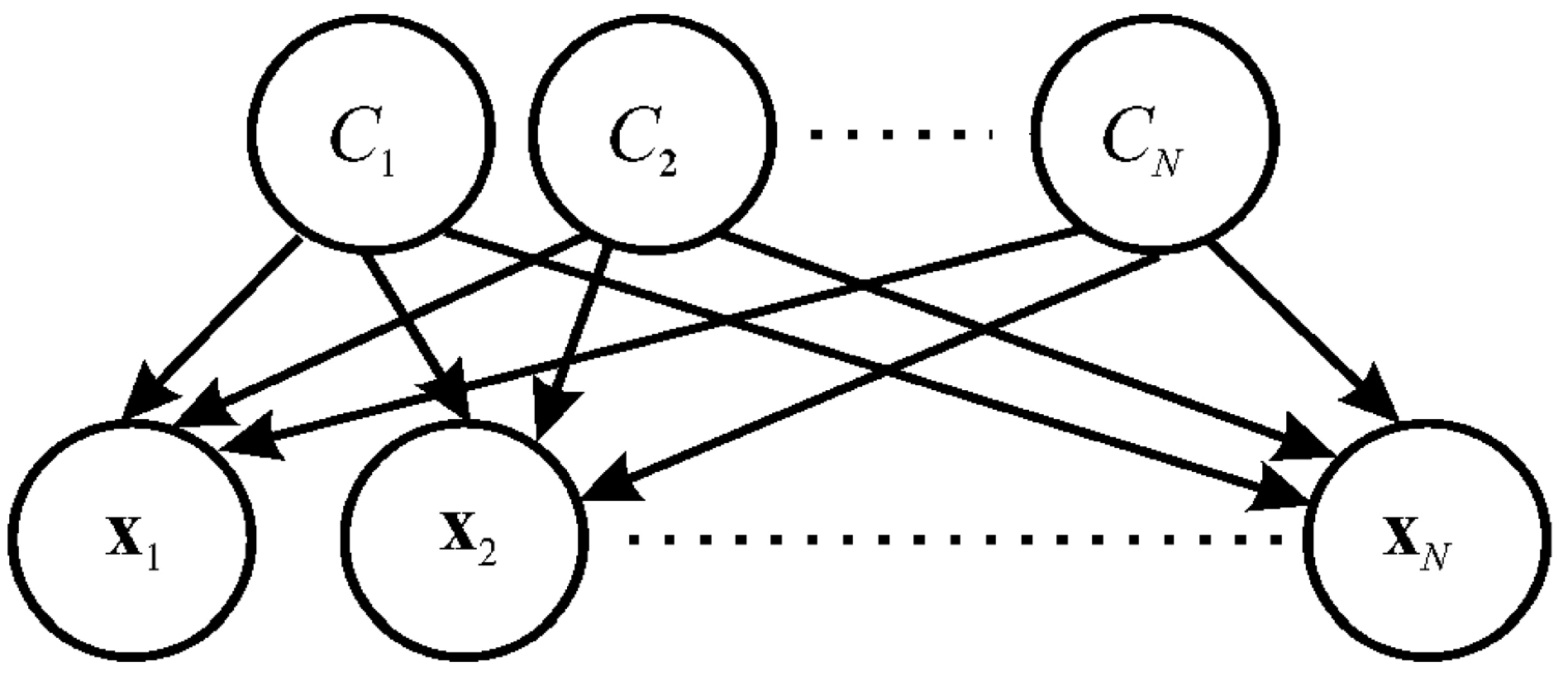
Figure 2.
Ranges of financial data for implementing Section 4.3
Figure 2.
Ranges of financial data for implementing Section 4.3
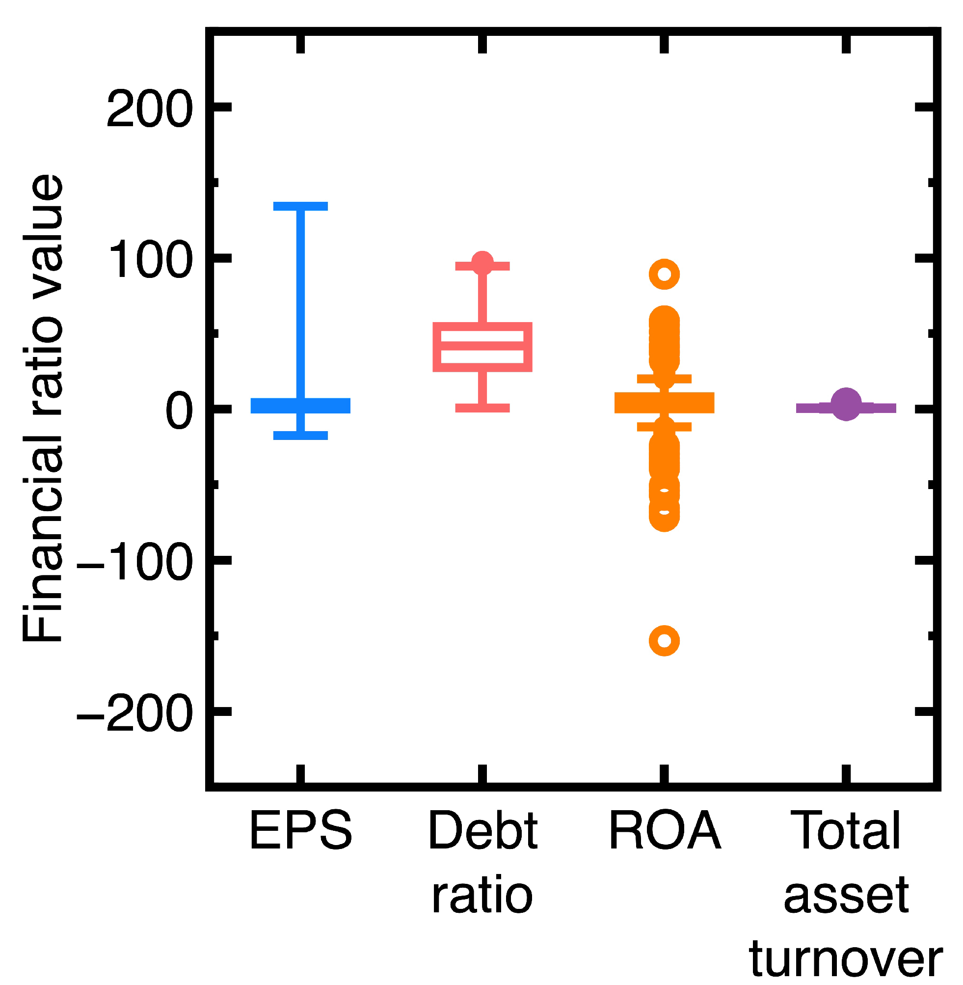
Figure 3.
Resulting ROC curves of Section 4.1
Figure 3.
Resulting ROC curves of Section 4.1
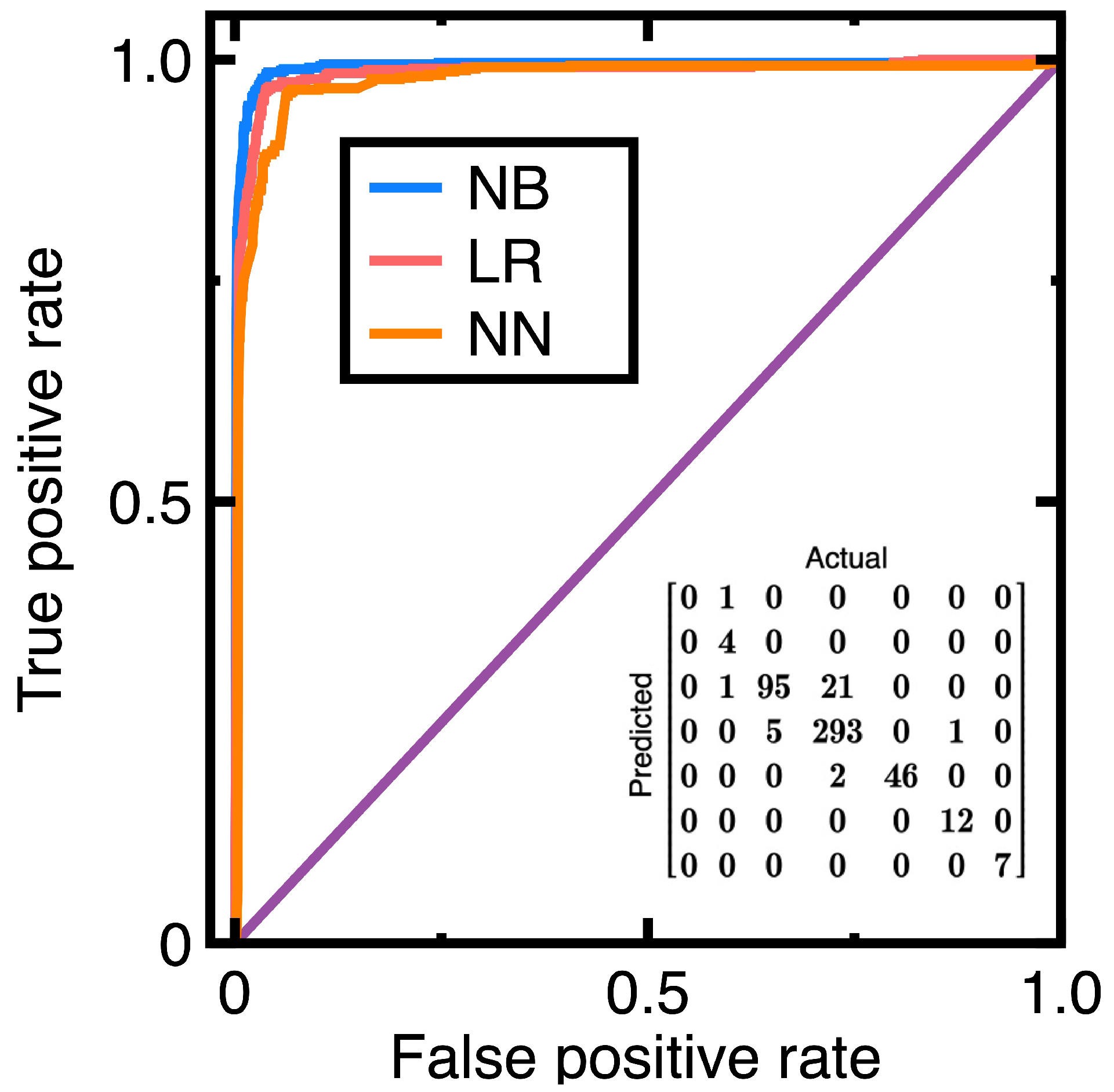
Figure 4.
Identification of targets with assumed financial health deterioration between the fourth quarter of 2023 and the first quarter of 2024
Figure 4.
Identification of targets with assumed financial health deterioration between the fourth quarter of 2023 and the first quarter of 2024
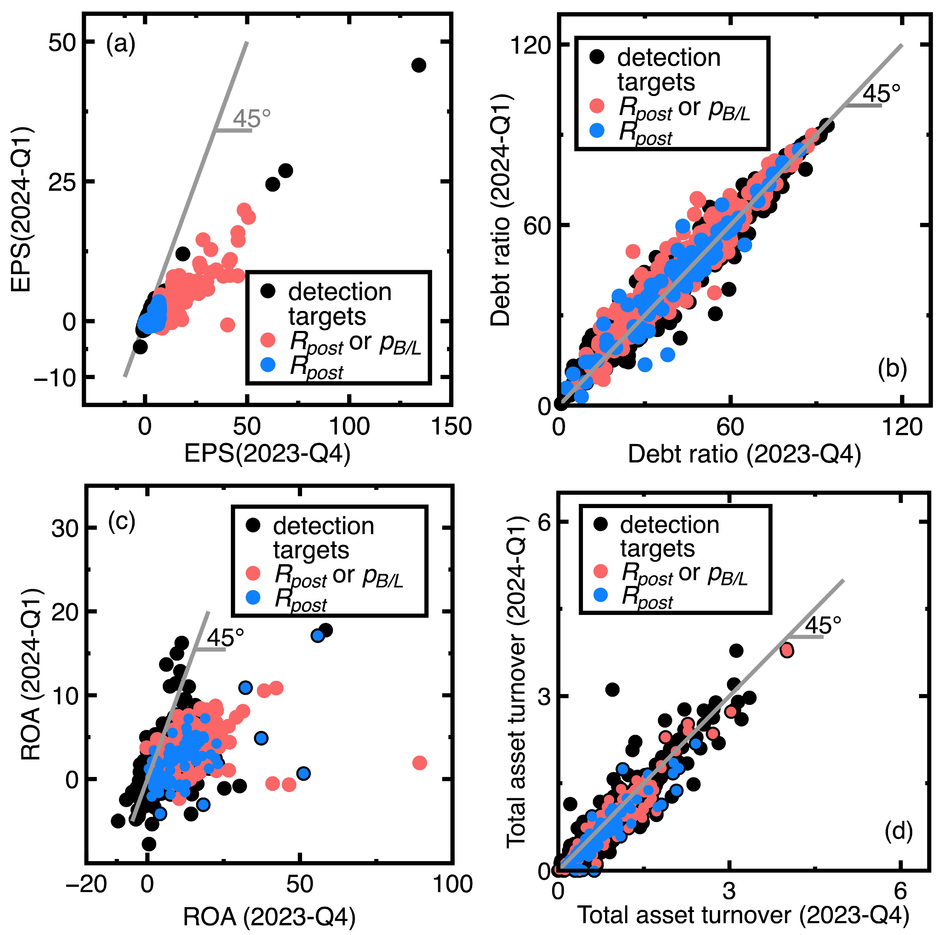
Figure 5.
Ranges of financial data for implementing Section 4.2
Figure 5.
Ranges of financial data for implementing Section 4.2
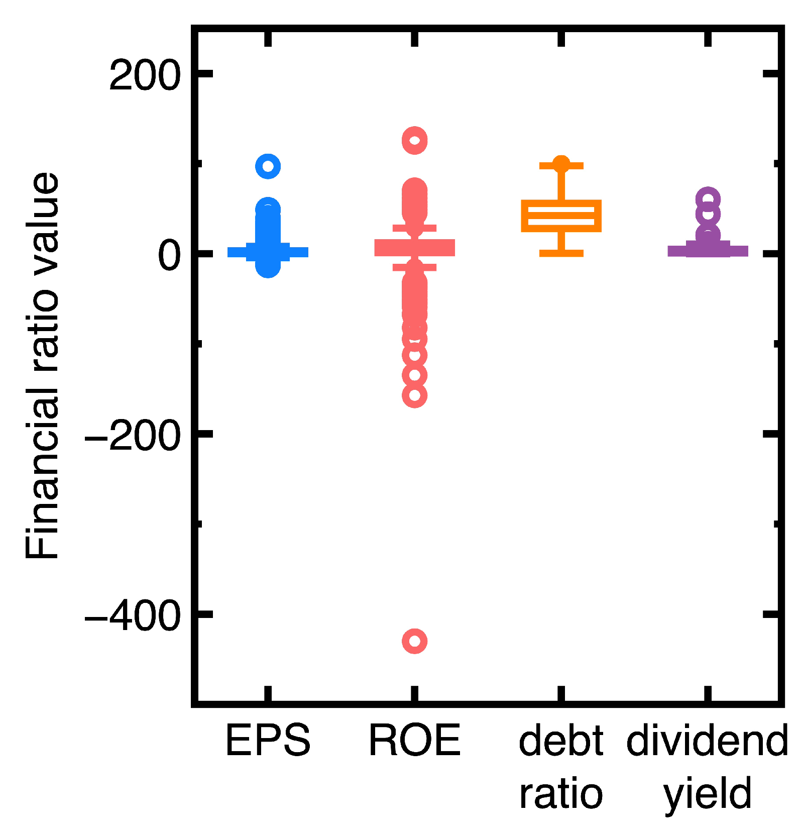
Figure 6.
Resulting ROC curves in the second experiment
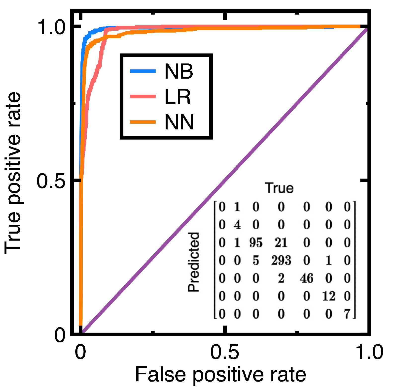
Figure 7.
Identification of companies with assumed financial health deterioration between the third and fourth quarters of 2023
Figure 7.
Identification of companies with assumed financial health deterioration between the third and fourth quarters of 2023
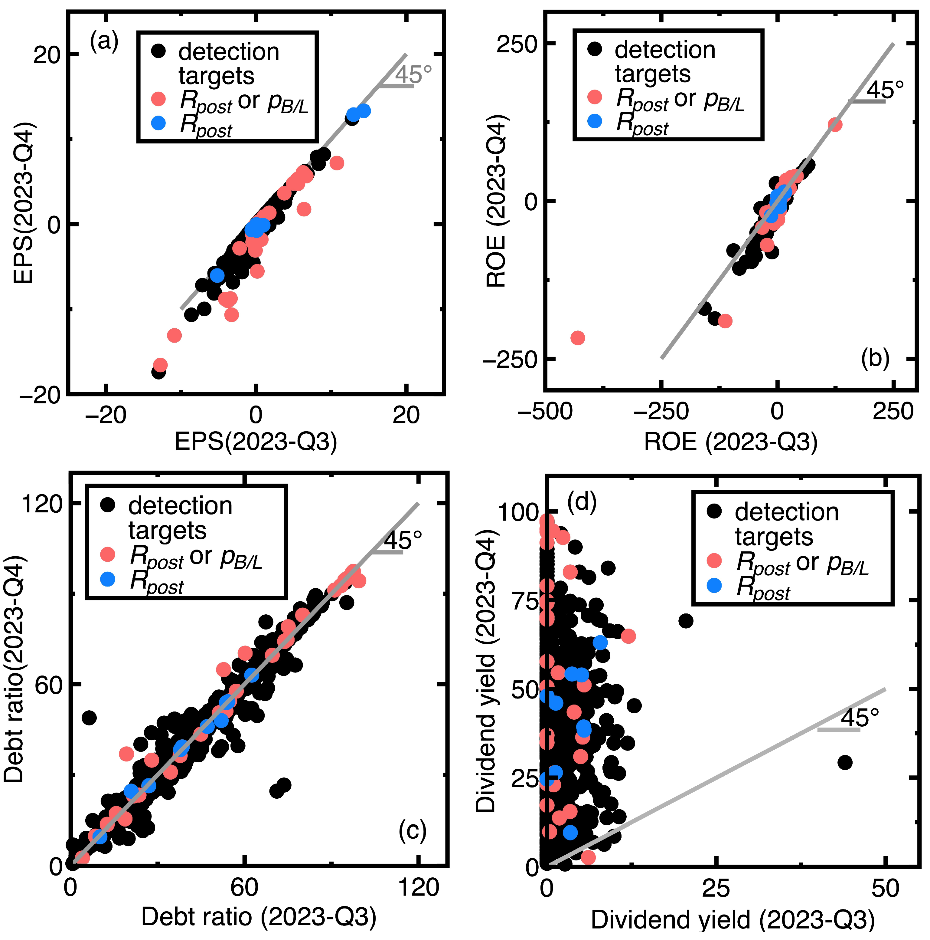
Figure 8.
Ranges of financial data for implementing Section 4.3
Figure 8.
Ranges of financial data for implementing Section 4.3
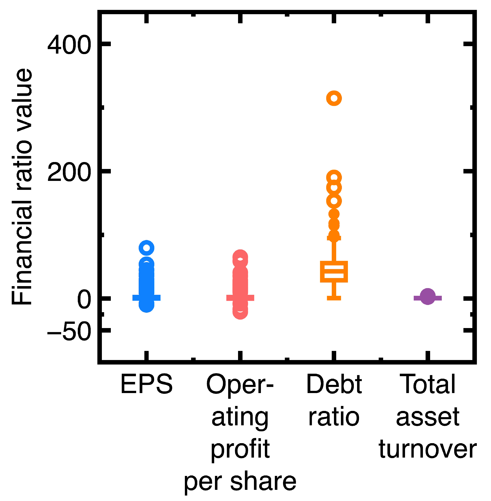
Figure 9.
Resulting ROC curves in the third experiment
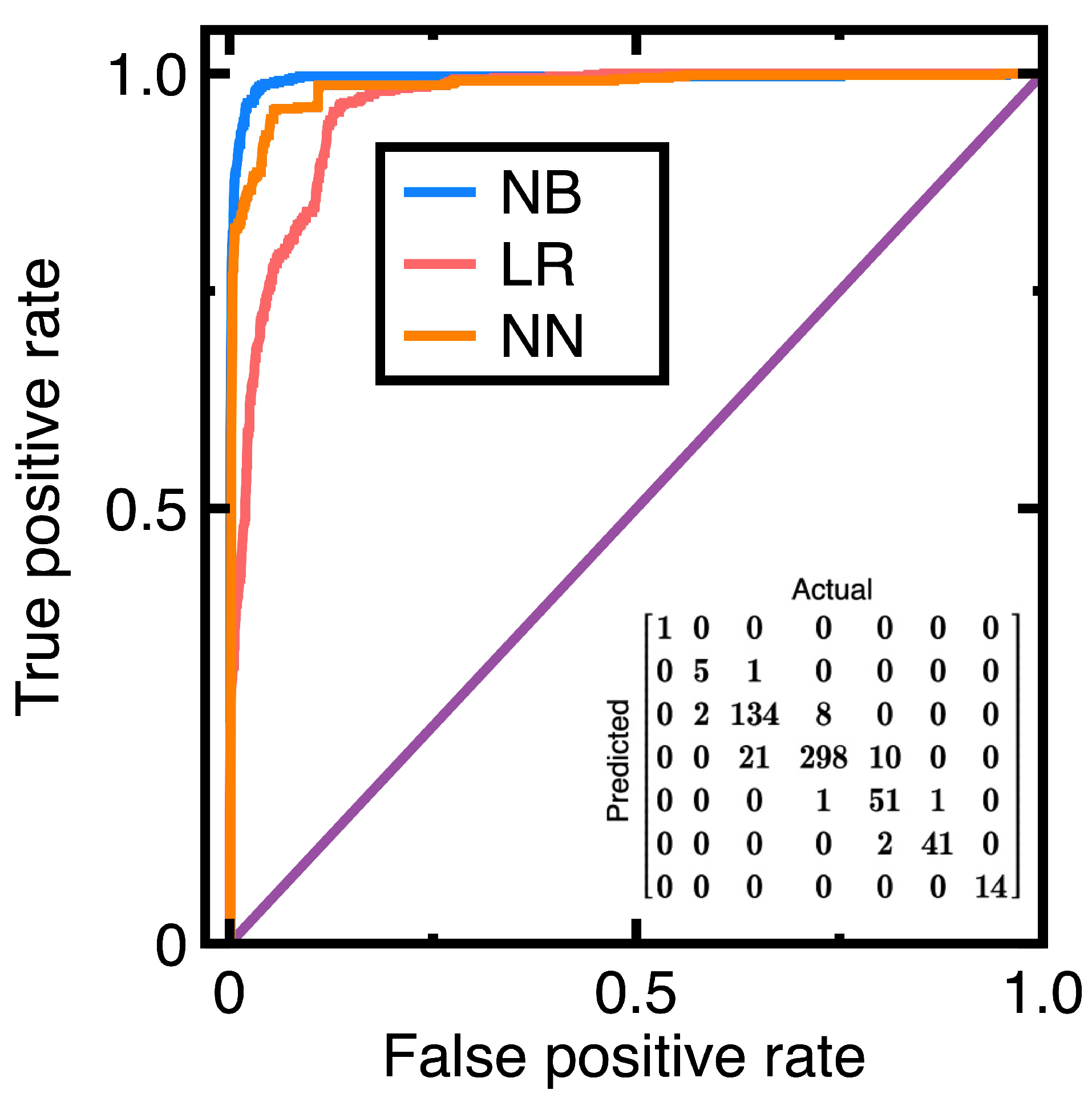
Figure 10.
Identification of companies with assumed financial health deterioration between the second and third quarters of 2024
Figure 10.
Identification of companies with assumed financial health deterioration between the second and third quarters of 2024
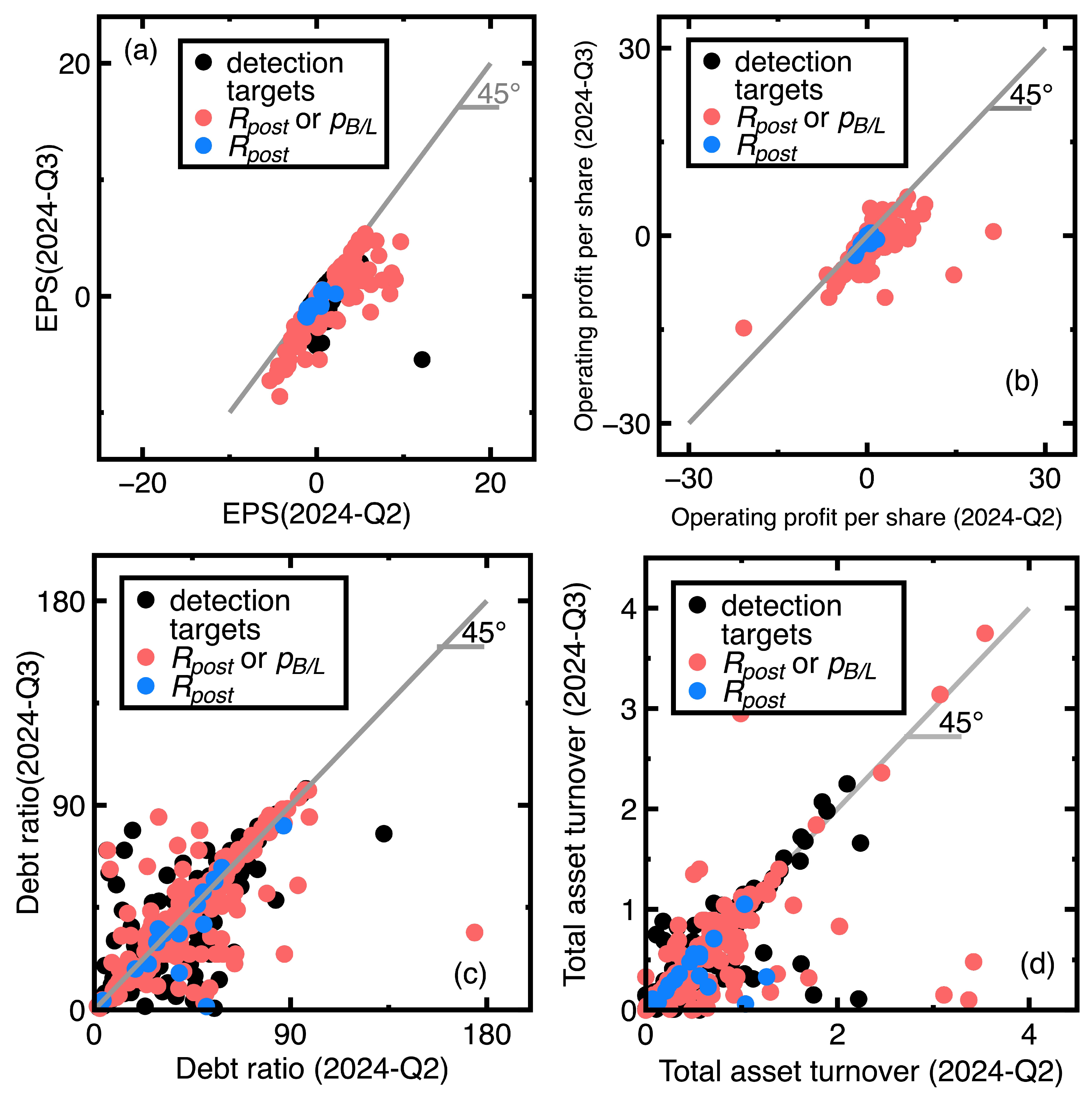

Table 1.
Metrics for describing the classification accuracy in the first experiment
| Metric | Weighted averaged Value |
|---|---|
| Accuracy | 0.949 |
| Precision | 0.921 |
| Recall | 0.954 |
| Specificity | 0.985 |
| F1 score | 0.936 |
Table 2.
Metrics calculated based on the confusion matrix shown inside Figure 6
Table 2.
Metrics calculated based on the confusion matrix shown inside Figure 6
| Metric | Weighted averaged Value |
|---|---|
| Accuracy | 0.936 |
| Precision | 0.937 |
| Recall | 0.936 |
| Specificity | 0.922 |
| F1 score | 0.935 |
Table 3.
Metrics calculated based on the confusion matrix shown inside Figure 9
Table 3.
Metrics calculated based on the confusion matrix shown inside Figure 9
| Metric | Weighted averaged Value |
|---|---|
| Accuracy | 0.92 |
| Precision | 0.926 |
| Recall | 0.92 |
| Specificity | 0.967 |
| F1 score | 0.922 |
Disclaimer/Publisher’s Note: The statements, opinions and data contained in all publications are solely those of the individual author(s) and contributor(s) and not of MDPI and/or the editor(s). MDPI and/or the editor(s) disclaim responsibility for any injury to people or property resulting from any ideas, methods, instructions or products referred to in the content. |
© 2024 by the authors. Licensee MDPI, Basel, Switzerland. This article is an open access article distributed under the terms and conditions of the Creative Commons Attribution (CC BY) license (https://creativecommons.org/licenses/by/4.0/).
Copyright: This open access article is published under a Creative Commons CC BY 4.0 license, which permit the free download, distribution, and reuse, provided that the author and preprint are cited in any reuse.


