
Submitted:
31 March 2025
Posted:
01 April 2025
You are already at the latest version
Abstract
With its fast advancements, Cloud Computing opens many opportunities for research in various applications from the robotics field. In our paper, we further explore the prospect of integrating Cloud AI object recognition services into an industrial robotics sorting task. Starting from our previously implemented solution on a digital twin, we are now putting our proposed architecture to the test in the real world, on an industrial robot, where factors such as illumination, shadows, different coloring and textures of the materials influence the performance of the vision system. We compare the results of our suggested method with the ones from an industrial machine vision software, obtaining promising performance, opening additional application perspectives in the robotics field as Cloud and AI technology continuously improves.
Keywords:
ABB RobotStudio
; industrial robots
; Cloud Computing
; object recognition
; Microsoft Azure Custom Vision
; computer vision
; Digital Twin
1. Introduction
The desire to improve the performance of manufacturing processes led to the emergence of many novel approaches to keep up with the rapidly evolving world of robotics, one of them being Cloud Robotics [1]. Moving the computationally intensive tasks to the cloud, enhances the system’s performance and computational capabilities, mitigating the known limitations of robotic devices, (some notable examples being the limited storage and on-board computation, as well as battery and storage capacities), while offering a way of sharing services [2].
In our previous article [4], we utilized a Digital Twin [3] from ABB RobotStudio in order to test the performance of our proposed solution in a simulated environment before implementing it on the real robot. In this article, we take the proposed architecture from our previous work and compare the results we obtained there in Robot Studio with the ones we obtain now, in the real world, using the ABB IRB 140 industrial robot. We compare the performance obtained with the proposed method, based on Custom Vision, with a commercial machine vision software used in industrial applications. Custom Vision is part of Microsoft Azure’s AI services and it allows users to create, train and evaluate their own models for image classification or object detection and recognition. We particularly suggest this method as a fallback option for cases where specialized machine vision software is unable to detect the objects, such as when they are dirty or overlapping.
Various types of AI techniques are being used by the scientific community for classification and detection tasks [5,6,7]. In the paper [8], cloud technology is used in a face recognition application based on Deep Learning algorithms in order to improve the speed and overcome robot on board limitations. They had encrypted the images used for training and testing, and tried several deep learning algorithms for training, in order to measure and compare the security, time complexity, and the accuracy of the recognition for the algorithms in the cloud and on the robot, obtaining the overall best security and recognition accuracy with the genetic algorithm. Their results show that by using the cloud environment compared to performing the same computation for the same algorithm directly on the robot, the recognition time is decreased from 0.559 seconds to 0.014 seconds, while maintaining the performance of the algorithm. Therefore, this paper showcases Cloud’s ability to decrease the computation time of resource intensive robotics tasks.
The paper [9] presents an autonomous pick-and-sort operation in industrial cloud robotics based on object recognition and motion planning. The object recognition uses a CNN and for performing the training, cloud computing resources were utilized to meet the high computational resources needs. The CNN method, compared to a CG algorithm, improved the object recognition time by a factor of 10. This application has a similar use case with ours, since they are also executing a pick-and-sort operation using an industrial robot. Their results showed that for a mean inter-object spawning time of 14 seconds and a mean service time needed for the robot arm to perform the movement of 13 sec, the pick-and-sort operation could reach 71.3% overall success rate.
Cloud Computing plays an important role in future internet-based solutions, supporting the evolution of technology trough innovations such as the development of smart cities [10] or collaborative computing [11]. We see that various cloud-based solutions are being approached by researchers for various robotics applications, at different levels of the architecture, while at the same time efforts are being put into improvements on resources [12], workload balancing abilities [13] and the consistency of connectivity of the Cloud.
In particular, the paper [14] focusses on improving the load balancing abilities of the Cloud. They propose a solution to increase the computation performance and resource usage efficiency of the platform by enhancing the resources management module with the use of a flexible container capacity scheduling algorithm. The algorithm performs capacity elastic scheduling operations based on the usage of CPU, memory and network of the containers. This paper shows how consistent research efforts channeled towards the load balancing abilities of the Cloud while multiple robots have access to the cloud service on demand, could increase the collaborative capabilities of robots.
Another area which is receiving attention is the consistency of the connectivity. For example, in [15] an IoRT and cloud robotics solution is proposed based on a three-level client server architecture. Django was utilized for the development of the AWS Cloud hosted application, demonstrating real-time, bidirectional communication capabilities. They tested the solution on several physical and simulated robots and obtained good capabilities for long distance global remote control and monitoring using the Internet, while confirming the robustness of the framework, and obtaining minimal communication delays with good performance in both local and cloud environments.
The paper [16] discusses the advancements in addressing issues such as low latency, the scalability of the data storage, computation and resource management efficiency through the incorporation of AI based optimization, cloud services and workload management strategies, to enhance the Internet-driven applications.
While the capabilities of Could platforms increase and further improvements are being made relating to their resources, workload balancing ability and the consistency of connectivity between users or devices, we expect to see them integrated in robotics solutions more and more often.
In the remaining of the paper, we will present our architecture with its constituent components, how the implementation was achieved, the results obtained for two illumination conditions (natural light vs artificial light) and for both solutions (the proposed solution based on Custom Vision vs the industrial machine vision software) as well as our conclusions, after analyzing the results.
2. Materials and Methods
Our suggested solution for the sorting task incorporates Microsoft Azure Custom Vision, a cloud service that enables the localization (obtaining the position) and identification (obtaining the type) of items in a picture using a user-created custom model. The position is denoted by a bounding box in which the object is contained, and the type is represented by a tag and a detection confidence returned by the service. The model was trained using 40 images, taken by the camera in good illumination conditions, with plenty of natural light, of 5 objects of different shapes and colours (a black circle, a purple square, a green rhombus, a yellow trapezoid and a red hexagon), placed in different positions and orientations. The training is performed by assigning bounding boxes and tags for the objects present in the training images, and then an ONNX model is computed by the service. The result of the training process can be seen in Figure 1.
The layout of the system is made up of an industrial robot, the IRB 140 from ABB, the vision system, an Ace2 R a2A2590-22gcBAS [17] camera from Basler with a C125-1620-5M f16mm lens [18], the Microsoft Azure Custom Vision cloud service and the computer that acts as an interface between the previously mentioned components, as it can be seen in Figure 2. The same system is presented in Figure 3 (a), where the vacuum suction gripper used for manipulating the objects is highlighted.
The computer is the center piece of the system. It runs a Python script that connects to the camera via a GigE connection, using the Basler pyPylon wrapper and requests images from the camera. The vision system, upon receiving a request, takes a picture and sends it back to the computer, where the same Python script creates a connection to the cloud and sends the pictures further to Microsoft Azure Custom Vision, over an API, and awaits a response. When the cloud service API response is received, it is processed and transmitted to the robot arm - robot controller pair for the sorting process.
Azure AI Custom Vision provides an API answer in JSON format that includes the kind of item identified, the position, indicated by a bounding box, and the detection probability. Following camera calibration, the object location in camera frame, in millimeters, is calculated using the pixel to millimeter ratio. Applying a coordinate system transform (Figure 3 (b)), the position of the handling point in the robot frame is obtained and finally transmitted to the robot controller over the Ethernet connection by the Python script. The coordinate system (P1P3P2), for the robot-camera calibration, is adjusted in the vision system based on the points that are learnt with the robot. For this, a special target (arrow) is used. The event diagram for the whole procedure can be seen in Figure 4.
Experiments have been done for a material handling task executed by the already introduced industrial robot, which uses guidance information from two sources:
- the proposed machine vision service, and
- a commercial machine vision software, namely MVTec Merlic
Both vision systems use the same acquisition solution, respectively a fixed network industrial camera (the GIGE type from Basler) which inspects the vision plane. The handling principle, presented in (Figure 3 (b)), uses the concept of workobject which is a reference frame used to define the position and orientation of a workpiece or fixture in space. In our case, the workobject is in the vision plane. The robot-camera or hand-eye calibration (ref) consists of:
- aligning the axis of the vision plane with the axis of the robot workobject, and
- overlaying the origin
In this respect, after applying the camera calibration described by the translation vector , the rotation matrix (Equations 1 and 2) and the pixel to mm ratio of , i.e. transforming the position from camera coordinates to the workobject coordinates, as illustrated in Figure 5, the vision system offers information in mm about the location of the recognized handled object in the learnt workobject. This information is used to perform the handling of the object.
The workobject is defined by the translation vector t and the rotation quaternions q as seen in Equation 3. The transformation matrix T is computed as Equation 4 and can be used to transform a point from the vision plane to the robot plane as shown in Equation 5, where is the point in the vision plane, is the point in the robot plane. The inverse operation can be performed like in Equation 6 using the inverse of the transformation matrix , seen in Equation 7.
The experiments consist in evaluating the robot-vision accuracy through both methods, Microsoft Azure Custom Vision and MVTec Merlic, compare the results and see how the cloud service performs against the industrial solution. A robot trajectory has been implemented, which uses 12 points on the vision plane. The robot will put the test target (which can be one of the five objects) on the vision plane and the coordinates will be stored. The target will be left on the vision plane, and its position will be computed using the vision system. The image processing time is also measured at the consumer side, from the time a command is issued to the moment the result is received (i.e. from the time the image is sent to the cloud, to the moment the results are received). For each object, 12 experiments have been performed, under different illuminations, first in similar conditions as the images used for training, i.e. with natural light and then under artificial light. The difference in lighting can be seen in Figure 6 Comparative results are illustrated in the next section.
3. Results
The position of the objects, which are compared in this section, represents the center of the bounding box containing the objects as seen in Figure 7, and is also the picking point for handling the object.
A screenshot of the bounding boxes and tags for object that have been identified by the industrial solution is presented in Figure 12. The tool for identification is called Deep Learning AI - Find Objects and uses an NN computed by MVTec Deep Learning Tool, trained in a similar manner as the cloud solution, using the same 40 images of the objects, for which bounding boxes and tags were assigned.
In Table 1 and Table 3, 10 experiments are presented for each system, 5 experiments done under natural light and 5 under artificial light, with one of each type of object. The detection confidence is displayed as provided by the vision system, the errors represent the position difference in millimeters, in the vision plane, from the placing point, as used by the industrial robot, and the pick point returned by the vision system, and finally, the time represents the duration of the image processing in seconds or milliseconds, from the moment the image is sent to the vision system, to the moment the results are received.
In Table 2 and Table 4 the mean values and SD are illustrated, in the same conditions as previously, obtained for each system. For this analysis, 12 experiments have been performed for each object, placed in different positions, and under both types of ilumination, adding up to a total of 120 experiments.
In Table 2 it can be observed that the lowest Detection Confidence, when using the cloud service, is obtained for the Rhombus, under Artificial light, with a mean of 0.63 and an SD of 0.13, while the best Detection Confidence is gained for the naturally illuminated Circle , with a mean of 0.93 and an SD of 0.03. In terms of positioning error, the biggest error is seen when detecting the Trapezoid, having a mean error on X axis of 3.00mm with an SD of 2.19mm, and a mean error on Y axis of 3.13mm with an SD of 1.35mm. The smallest errors can be seen in the detection of the Circle, with errors of 0.53mm on X axis and 0.61mm on Y axis, along with SDs of 0.37mm on X axis and 0.53mm on Y axis.
A similar case can be seen in Table 4, for the industrial application, with the smallest errors for the detection of the Circle, of 0.66mm mean error on X axis and 0.4mm SD and 0.48mm mean error on Y axis and 0.29mm SD, and the biggest error for the Trapezoid, with 3.05mm mean and 1.69mm SD on X axis, and 2.89mm mean and 1.86 SD on Y axis. The confidence in this case varies very little, with almost all cases having a confidence of 1, except for the Square and Trapezoid, which have reduced values when illuminated by artificial light.
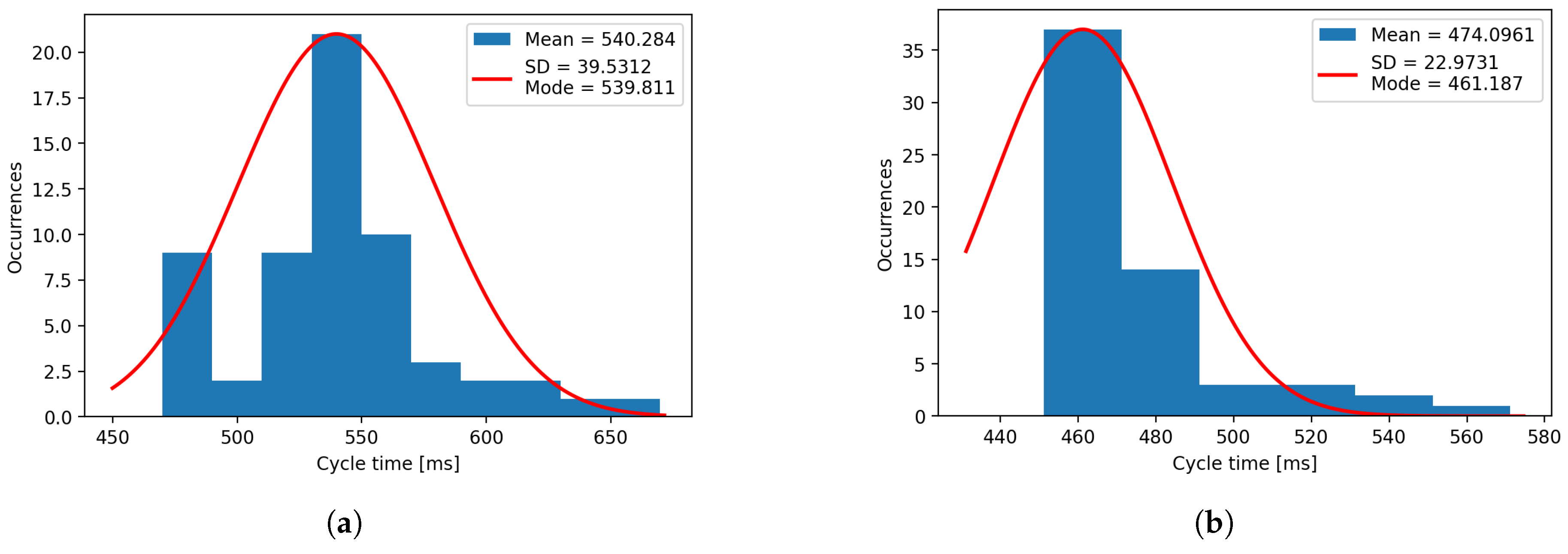
Regarding the response time, for both systems, the results are consistent and don’t vary much with the object type or ambient light. In the case of the cloud system, the response time varies from a mean of 2.55 sec and an SD of 0.14sec in the case of the artificially illuminated Hexagon, to a mean of 2.94 sec and an SD of 0.39 sec for the naturally illuminated Circle. The industrial software offers a response in about 500ms in all cases, with the lowest average value being for the artificially lightened Square (mean of 472.6ms and SD of 27.7ms) and the highest mean value for the naturally lightened Trapezoid (mean of 564.6ms and SD of 37.3ms).
Using the data extracted from the same experiments, histograms for confidence (Figure 8 and Figure 13), error on ‘X’ axis (Figure 9 and Figure 14), error on ‘Y’ axis (Figure 10 and Figure 15) and time (Figure 11 and Figure 16) have been plotted for both systems. It can be observed that the mean and mode varies heavily for the plotted histograms, which denotes that the distributions are sqewed, negative sqewed for the confidence, and positive sqewed for the errors, due to their limits. The confidence cannot exceed 100%, and the error cannot be less than 0mm.

Table 1.
Table presenting a part of the data obtained when using the cloud solution.
| Experiment Number | Ambient light | Object type | Detection Confidence | X Error [mm] | Y Error [mm] | Time [sec] |
|---|---|---|---|---|---|---|
| 1 | Natural | Circle | 0.95 | 0.13 | 1.80 | 3.50 |
| 2 | Natural | Square | 0.95 | 1.97 | 1.41 | 2.78 |
| 3 | Natural | Rhombus | 0.87 | 1.87 | 1.83 | 2.57 |
| 4 | Natural | Trapezoid | 0.96 | 0.10 | 2.90 | 2.57 |
| 5 | Natural | Hexagon | 0.82 | 0.17 | 0.30 | 2.45 |
| 6 | Artificial | Circle | 0.86 | 0.66 | 0.52 | 2.40 |
| 7 | Artificial | Square | 0.92 | 2.77 | 1.89 | 2.37 |
| 8 | Artificial | Rhombus | 0.78 | 0.65 | 0.81 | 2.87 |
| 9 | Artificial | Trapezoid | 0.79 | 0.63 | 3.45 | 2.45 |
| 10 | Artificial | Hexagon | 0.90 | 1.37 | 4.30 | 2.40 |
Table 2.
The mean and standard deviation for the confidence, error and response time, for all types of object in different type of light, for the cloud product.
Table 2.
The mean and standard deviation for the confidence, error and response time, for all types of object in different type of light, for the cloud product.
| Ambient light | Object type | Detection Confidence Mean / SD | X Error [mm] Mean / SD | Y Error [mm] Mean / SD | Time [sec] Mean / SD |
|---|---|---|---|---|---|
| Natural | Circle | 0.93 / 0.03 | 1.04 / 0.62 | 1.71 / 0.92 | 2.94 / 0.39 |
| Natural | Square | 0.90 / 0.08 | 1.78 / 1.04 | 1.49 / 0.99 | 2.64 / 0.19 |
| Natural | Rhombus | 0.68 / 0.17 | 1.47 / 1.23 | 1.46 / 1.03 | 2.57 / 0.20 |
| Natural | Trapezoid | 0.85 / 0.20 | 2.9 / 1.79 | 1.84 / 1.04 | 2.57 / 0.14 |
| Natural | Hexagon | 0.89 / 0.05 | 2.50 / 1.85 | 2.05 / 1.41 | 2.64 / 0.15 |
| Artificial | Circle | 0.93 / 0.03 | 0.53 / 0.37 | 0.61 / 0.53 | 2.60 / 0.25 |
| Artificial | Square | 0.92 / 0.02 | 1.97 / 1.16 | 1.48 / 0.96 | 2.68 / 0.31 |
| Artificial | Rhombus | 0.63 / 0.13 | 2.06 / 1.00 | 1.46 / 0.91 | 2.65 / 0.26 |
| Artificial | Trapezoid | 0.66 / 0.11 | 3.00 / 2.19 | 3.13 / 1.35 | 2.75 / 0.44 |
| Artificial | Hexagon | 0.70 / 0.15 | 2.57 / 1.59 | 1.90 / 1.10 | 2.55 / 0.14 |
Figure 8.
(a) Confidence histogram for natural light. (b) Confidence histogram for artificial light.
Figure 8.
(a) Confidence histogram for natural light. (b) Confidence histogram for artificial light.
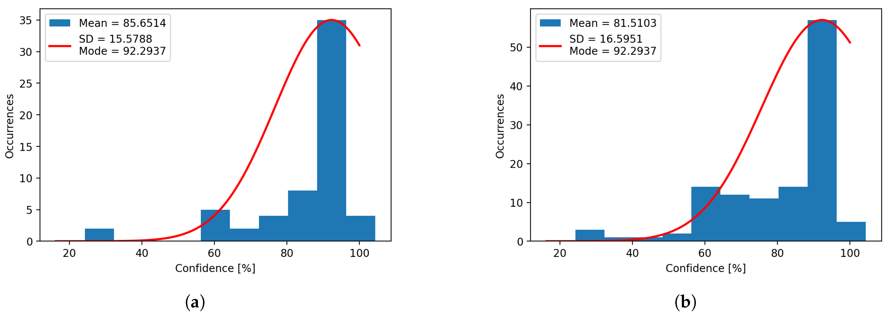
Figure 9.
(a) Error histogram on X axis for natural light. (b) Error histogram on X axis for artificial light.
Figure 9.
(a) Error histogram on X axis for natural light. (b) Error histogram on X axis for artificial light.
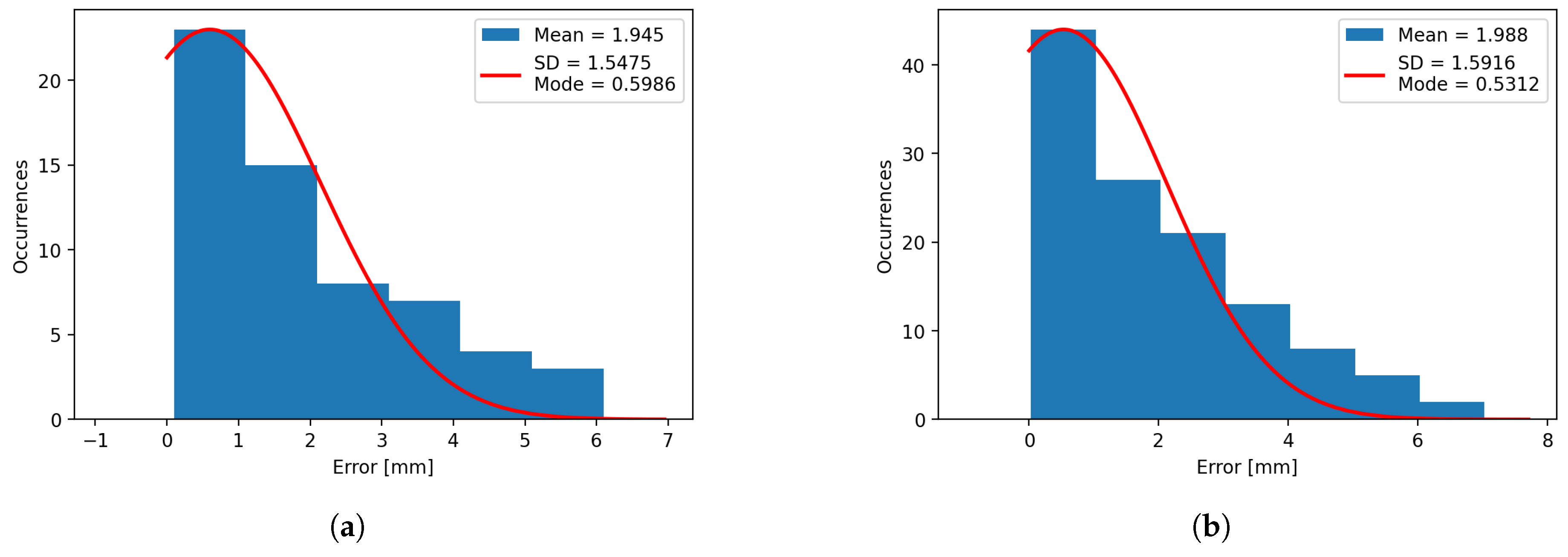
Figure 10.
(a) Error histogram on Y axis for natural light. (b) Error histogram on Y axis for artificial light.
Figure 10.
(a) Error histogram on Y axis for natural light. (b) Error histogram on Y axis for artificial light.
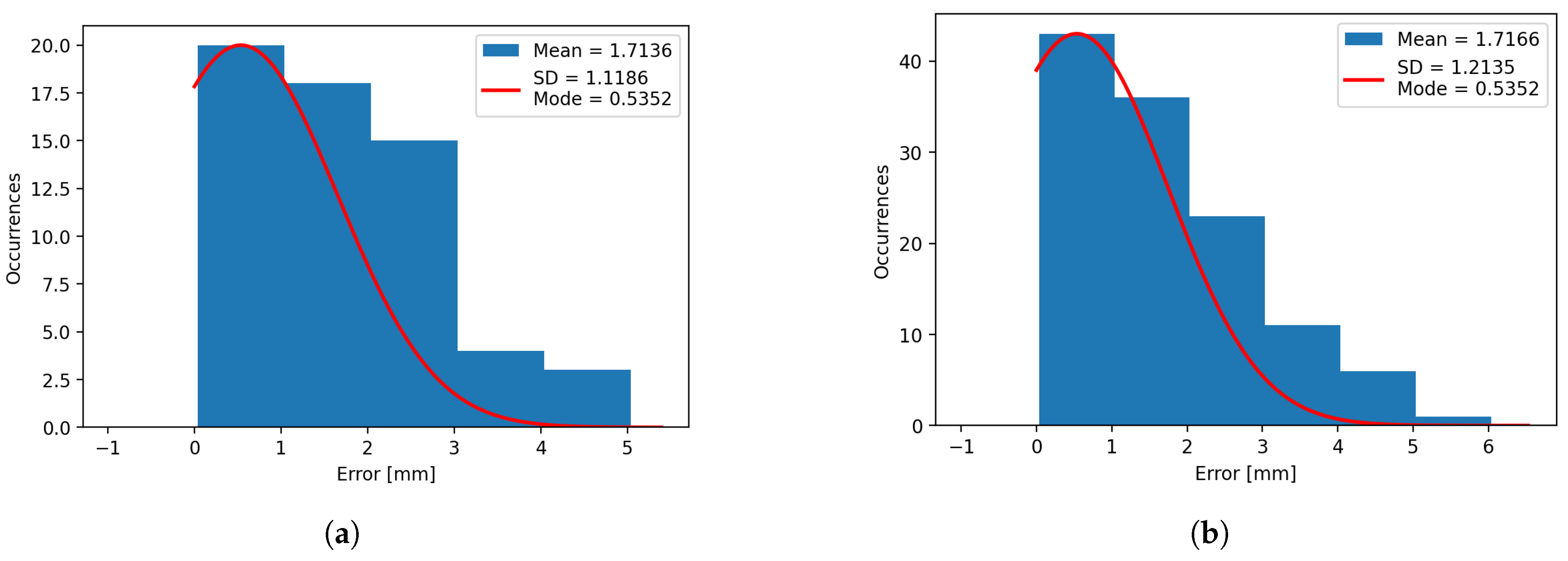
Figure 11.
(a) Time histogram for natural light. (b) Time histogram for artificial light.
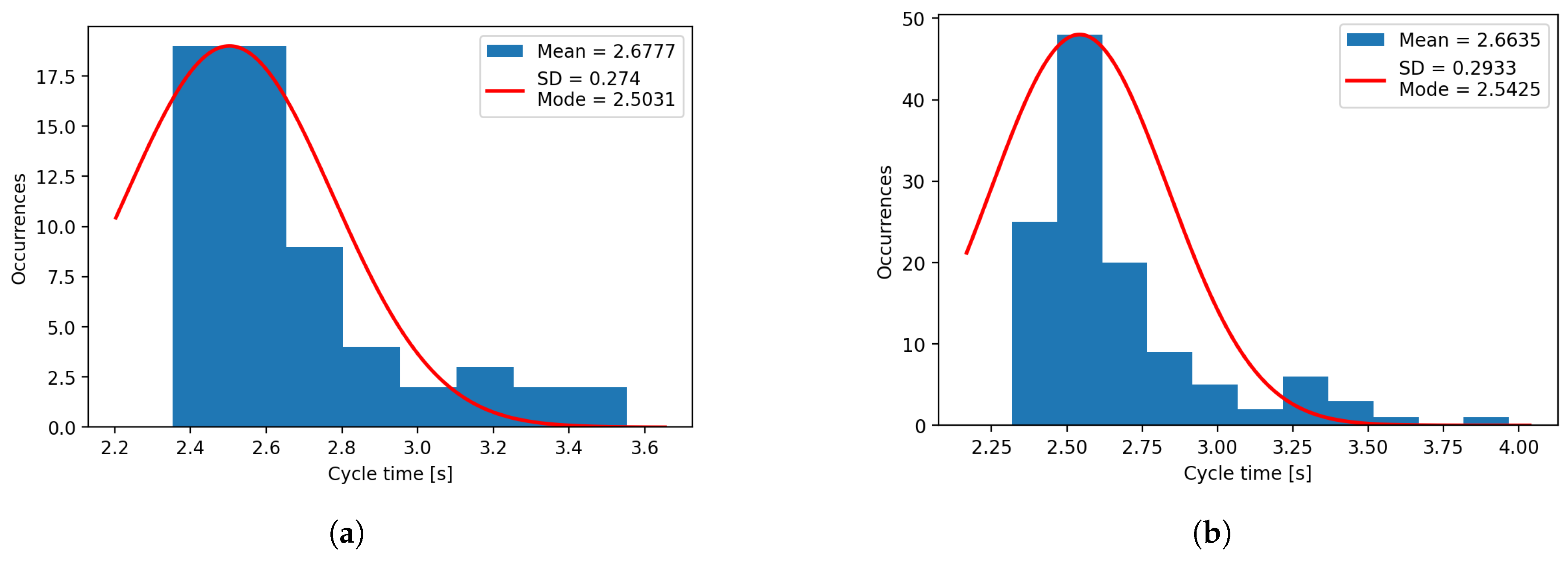
Figure 12.
Detected objects, as seen in MVTec Merlic.
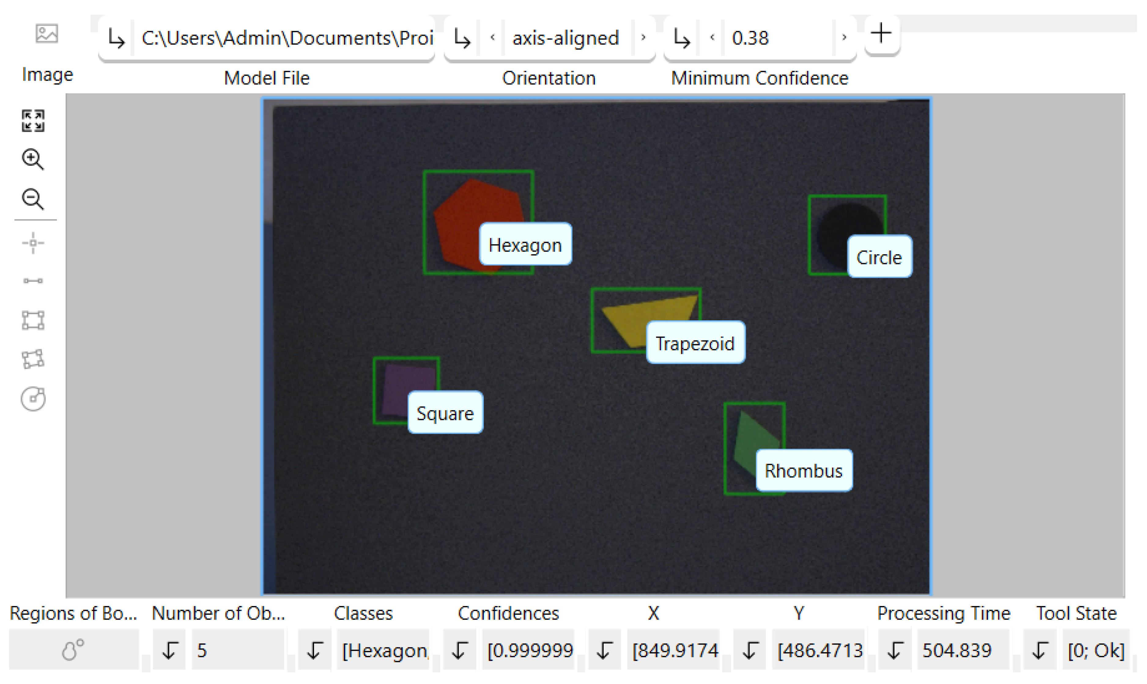
Table 3.
Table presenting a part of the data obtained when using the industrial solution.
| Experiment Number | Ambient light | Object type | Detection Confidence | X Error [mm] | Y Error [mm] | Time [ms] |
|---|---|---|---|---|---|---|
| 1 | Natural | Circle | 0.99 | 2.15 | 1.04 | 481.3 |
| 2 | Natural | Square | 0.99 | 2.73 | 1.83 | 563.8 |
| 3 | Natural | Rhombus | 0.99 | 4.28 | 0.46 | 528 |
| 4 | Natural | Trapezoid | 0.99 | 3.29 | 1.51 | 533.6 |
| 5 | Natural | Hexagon | 1 | 4.07 | 1.30 | 520.2 |
| 6 | Artificial | Circle | 1 | 0.36 | 0.28 | 467.5 |
| 7 | Artificial | Square | 0.99 | 2.88 | 0.97 | 463 |
| 8 | Artificial | Rhombus | 0.99 | 3.23 | 1.14 | 474.6 |
| 9 | Artificial | Trapezoid | 0.99 | 5.60 | 0.51 | 459 |
| 10 | Artificial | Hexagon | 0.99 | 3.53 | 0.86 | 532.1 |
Table 4.
The mean and standard deviation for the confidence, error and response time, for all types of object in different type of light, for the industrial software.
Table 4.
The mean and standard deviation for the confidence, error and response time, for all types of object in different type of light, for the industrial software.
| Ambient light | Object type | Detection Confidence Mean / SD | X Error [mm] Mean / SD | Y Error [mm] Mean / SD | Time [ms] Mean / SD |
|---|---|---|---|---|---|
| Natural | Circle | 0.99 / 0 | 1.75 / 0.77 | 1.13 / 1.01 | 484.5/ 13.9 |
| Natural | Square | 0.99 / 0 | 2.52 / 0.85 | 1.26 / 0.94 | 548.6 / 30.6 |
| Natural | Rhombus | 0.99 / 0 | 2.6 / 1.43 | 1.08 / 0.75 | 549.8 / 20.9 |
| Natural | Trapezoid | 0.99 / 0 | 3.05 / 1.69 | 2.56 / 1.85 | 564.6 / 37.3 |
| Natural | Hexagon | 1 / 0 | 2.49 / 1.96 | 1.84 / 1.11 | 553.6 / 28.3 |
| Artificial | Circle | 1 / 0 | 0.66 / 0.40 | 0.48 / 0.29 | 473.5 / 20 |
| Artificial | Square | 0.95 / 0.15 | 2.76 / 1.2 | 1.29 / 0.87 | 472.6 / 27.7 |
| Artificial | Rhombus | 0.99 / 0.01 | 2.47 / 1.07 | 1.1 / 1.02 | 467.4 / 18.4 |
| Artificial | Trapezoid | 0.97 / 0.06 | 2.89 / 2.48 | 2.89 / 1.86 | 473.9 / 22.4 |
| Artificial | Hexagon | 1 / 0 | 2.79 / 1.57 | 1.46 / 0.84 | 482.8 / 22.3 |
Figure 13.
(a) Confidence histogram for natural light, for the industrial software. (b) Confidence histogram for artificial light, for the industrial software.
Figure 13.
(a) Confidence histogram for natural light, for the industrial software. (b) Confidence histogram for artificial light, for the industrial software.
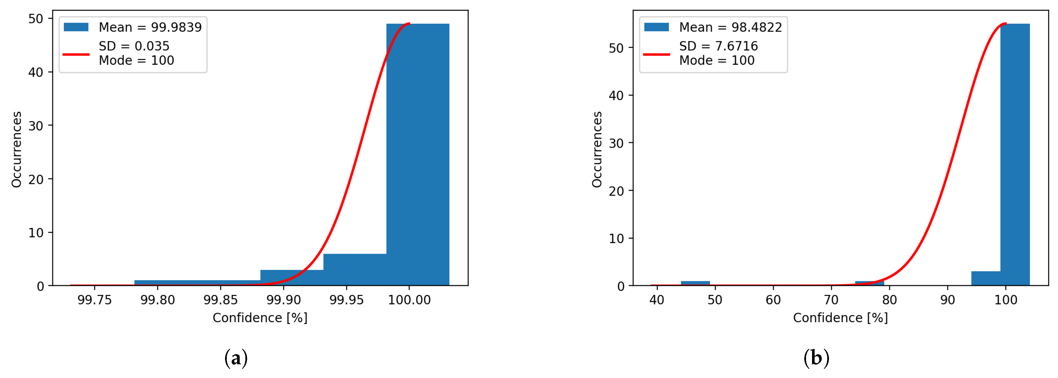
Figure 14.
(a) Error histogram on X axis for natural light, for the industrial software. (b) Error histogram on X axis for artificial light, for the industrial software.
Figure 14.
(a) Error histogram on X axis for natural light, for the industrial software. (b) Error histogram on X axis for artificial light, for the industrial software.
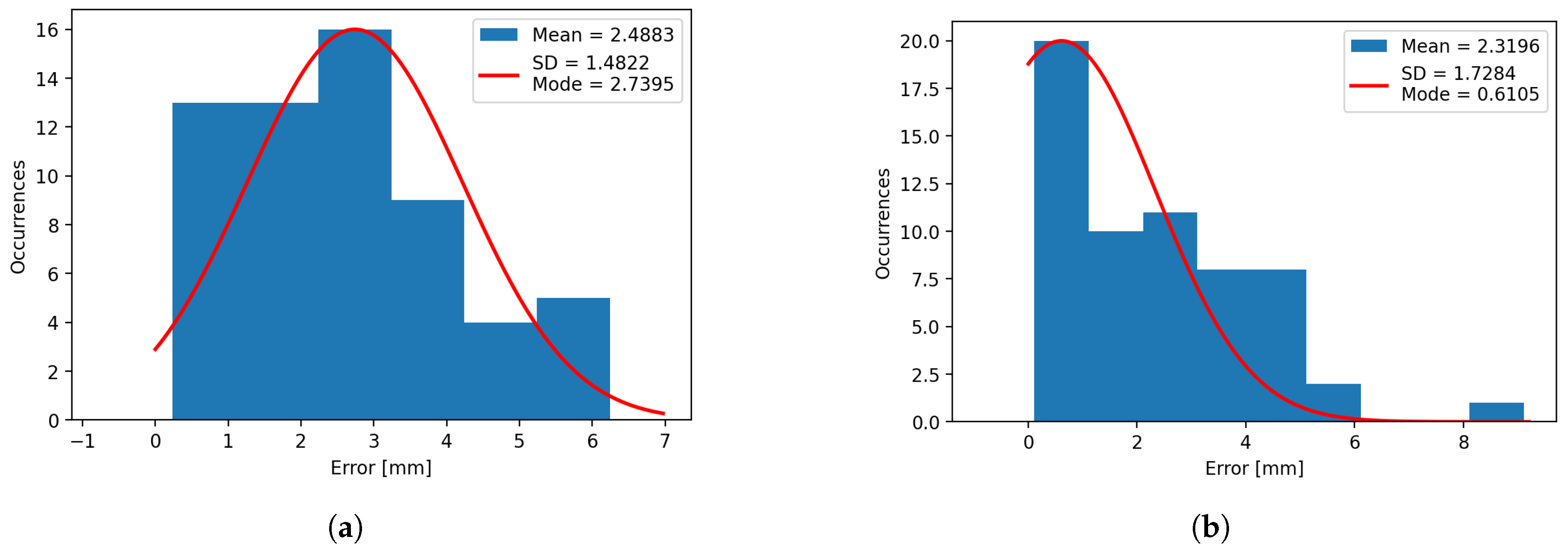
Figure 15.
(a) Error histogram on Y axis for natural light, for the industrial software. (b) Error histogram on Y axis for artificial light, for the industrial software.
Figure 15.
(a) Error histogram on Y axis for natural light, for the industrial software. (b) Error histogram on Y axis for artificial light, for the industrial software.
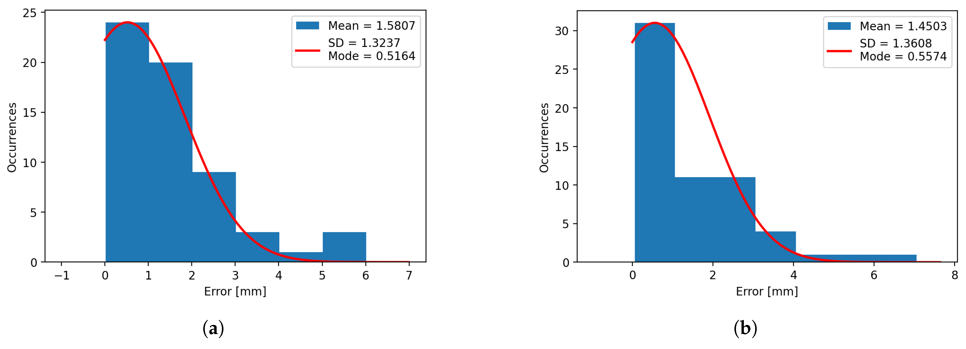
Figure 16.
(a) Time histogram for natural light, for the industrial software. (b) Time histogram for artificial light, for the industrial software.
Figure 16.
(a) Time histogram for natural light, for the industrial software. (b) Time histogram for artificial light, for the industrial software.
4. Discussion
When using the real-world system, the images taken contain several added noises: the image background (the table), the object’s texture, shadows, reflections and change in coloration due to the different light sources used, as compared to our previous work, where the images are taken inside a simulated environment. These noises decrease the detection confidence and increase the positioning error in the real environments, and may pose a problem when performing robot sorting operations.
The best results are obtained when using the natural light, under which the model was trained, and for the circular object, due to its symmetry.
Compared with the industrial software, the confidence in detection is reduced when using the cloud service, but the position errors remain similar. Regarding the response time, the local solution is faster, as to be expected, but the cloud response is not slow either.
The response time varies in regard with the internet speed, but it remains consistent under the same test conditions.
In comparison with classical identification methods, which take into account the shape and contour of the object, the presented method can be used successfully for identification in cases when the object are a bit dirty (Figure 17) or they overlap (Figure 18).
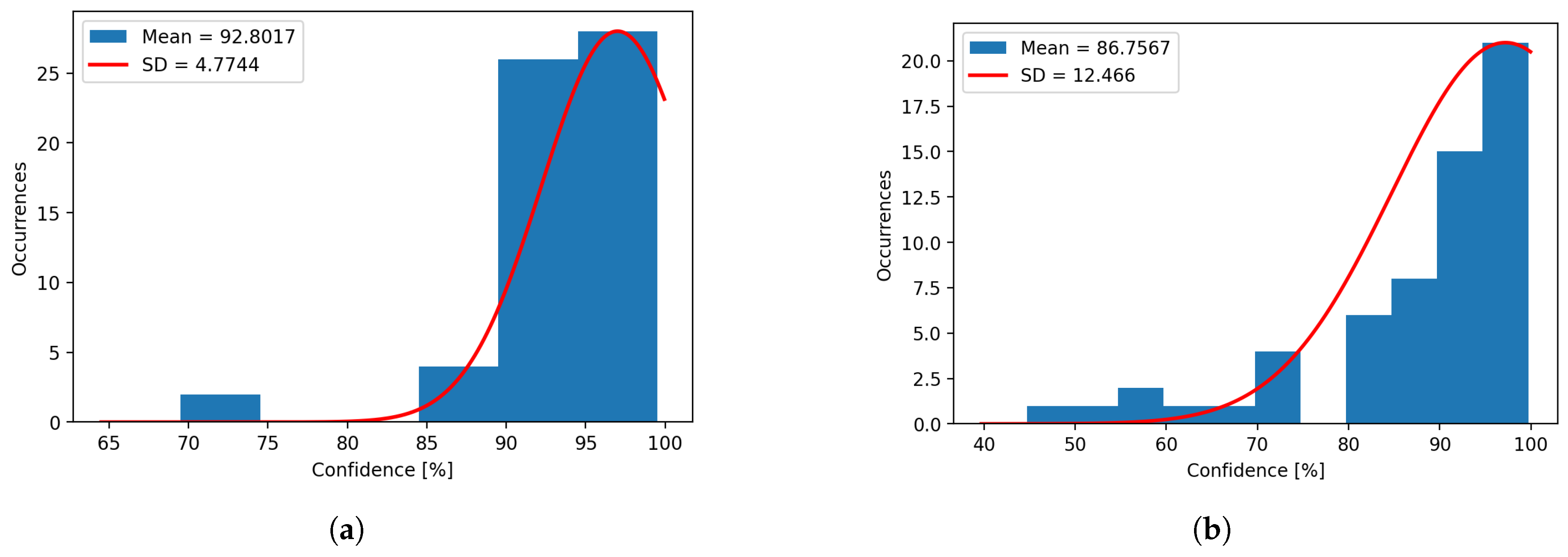
The results are better when using the industrial software, trained for the same images, but when using the detection images to improve the cloud solution model, the detection results are improving. In this case, we used the detection images with natural light to retrain and improve the model, obtaining the results presented in Figure 19 (a) for natural light, showing a 7.2% increase in detection confidence and Figure 19 (b) artificial light with a respectable 5.2% increase. Beside the increase in confidence, a reduction in standard deviation of 10.8% for natural light and 4.1% for artificial light is present.
5. Conclusions
The cloud service obtained the best results in natural illumination conditions, with good prediction confidences and sufficiently small errors to ensure object picking in every case. The implementation proved its overall connectivity consistency, while also demonstating robustness, providing good results in the case of partially dirty objects.
The prediction confidence calculated by the Custom Vision and MVTec Merlic are not directly comparable since the methods of calculation of the confidence are not transparent for either of them. Per our observation, after making additional tests, the confidence of MVTec Merlic for cases of correct prediction tends to be closer to the extremes (either very high, which happens for most cases, or in specific cases very low), we suspect that this behavior stems from the method used for calculating the confidence.
While the specialized software showed overall better and more consistent results, which is to be expected since it is a computer vision specifically made with industrial use in mind, the Custom Vision solution also performed satisfactory. These results open additional application perspectives in the robotics field with the quickly evolving AI technology and continuous increasing Cloud capabilities.
It is worth mentioning that Custom Vision’s lower limit of images for the training to take place is of 25, and the results compared were obtained for a training where we used 40 training images. We observed that for further training of the Custom Vision model with new images of the objects, its prediction confidence kept increasing. The point after which the confidence is not further increased by adding new images is still to be determined.
In the future, a system that combines the classical object identification, based on contour and edges with the NN based detection, used by the two systems that were compared in this work, can be developed to count for all the detection scenarios, In terms of light, background, overlap and dust to obtain the best overall results.
Author Contributions
Conceptualization, I.L.S. and A.M.; methodology, I.L.S., A.M. and S.R.; software, I.L.S., A.M. and I.L.; validation, I.L.S., A.M. and S.R.; formal analysis, I.L.S. and A.M.; investigation, I.L.S. and A.M.; resources, I.L.S., F.D.A. and S.R.; data curation, A.M.; writing—original draft preparation, I.L.S. and A.M.; writing—review and editing, I.L.S., A.M., I.L., S.R., F.D.A., D.C.P., and I.S.S.; visualization, A.M.; supervision, S.R., D.C.P. and I.S.S.; project administration, A.M.; funding acquisition, F.D.A., I.L.S. and A.M. All authors have read and agreed to the published version of the manuscript.
Funding
This research received no external funding.
Data Availability Statement
Dataset available on request from the authors.
Acknowledgments
This work was supported by the National Program for Research of the National Association of Technical Universities GNaC ARUT 2023, grant number 83/11.10.2023 (optDDNc).
Conflicts of Interest
The authors declare no conflicts of interest.
Abbreviations
The following abbreviations are used in this manuscript:
| AI | Artificial Intelligence |
| API | Application Programming Interface |
| AWS | Amazon Web Services |
| CG | Correspondence Grouping |
| CNN | Convolutional Neural Networks |
| CPU | Central Processing Unit |
| IoRT | Internet of Robotic Things |
| JSON | JavaScript Object Notation |
| NN | Neural Network |
| ONNX | Open Neural Network Exchange |
| SD | Standard Deviation |
References
- Dawarka, V.; Bekaroo, G. Building and evaluating cloud robotic systems: A systematic review. Robotics and Computer-Integrated Manufacturing, 2022, 73, p. 102240. [CrossRef]
- Zhang, H.; Zhang, L. Cloud Robotics Architecture: Trends and Challenges. 2019 IEEE International Conference on Service-Oriented System Engineering (SOSE), San Francisco, CA, USA, 04-09 April 2019, pp. 362–3625. [CrossRef]
- Fantozzi, I.C.; Santolamazza, A.; Loy, G.; Schiraldi, M.M. Digital Twins: Strategic Guide to Utilize Digital Twins to Improve Operational Efficiency in Industry 4.0. Future Internet 2025, 17, 41. [CrossRef]
- Stefan, I. L.; Mateescu, A.; Vlasceanu, I. M.; Popescu, D. C.; Sacala, I. S. Utilizing Cloud Solutions for Object Recognition in the Context of Industrial Robotics Sorting Tasks. 2024 International Conference on INnovations in Intelligent SysTems and Applications (INISTA), Craiova, Romania, 2024, pp. 1-6. [CrossRef]
- Roumeliotis, K.I.; Tselikas, N.D.; Nasiopoulos, D.K. Fake News Detection and Classification: A Comparative Study of Convolutional Neural Networks, Large Language Models, and Natural Language Processing Models. Future Internet 2025, 17, 28. [CrossRef]
- Sahnoun, S.; Mnif, M.; Ghoul, B.; Jemal, M.; Fakhfakh, A.; Kanoun, O. Hybrid Solution Through Systematic Electrical Impedance Tomography Data Reduction and CNN Compression for Efficient Hand Gesture Recognition on Resource-Constrained IoT Devices. Future Internet 2025, 17, 89. [CrossRef]
- Kamal, H.; Mashaly, M. Advanced Hybrid Transformer-CNN Deep Learning Model for Effective Intrusion Detection Systems with Class Imbalance Mitigation Using Resampling Techniques. Future Internet 2024, 16, 481. [CrossRef]
- Karri, C.; Naidu,M. S. R. Deep Learning Algorithms for Secure Robot Face Recognition in Cloud Environments. 2020 IEEE Intl Conf on Parallel & Distributed Processing with Applications, Big Data & Cloud Computing, Sustainable Computing & Communications, Social Computing & Networking (ISPA/BDCloud/SocialCom/SustainCom), Exeter, United Kingdom, 2020, pp. 1021-1028. [CrossRef]
- Zhang, Y.; Li, L.; Nicho, J.; Ripperger, M.; Fumagalli, A.; Veeraraghavan, M. Gilbreth 2.0: An Industrial Cloud Robotics Pick-and-Sort Application. 2019 Third IEEE International Conference on Robotic Computing (IRC), Naples, Italy, 2019, pp. 38-45. [CrossRef]
- Trigka, M.; Dritsas, E. Edge and Cloud Computing in Smart Cities. Future Internet 2025, 17, 118. [CrossRef]
- Souza, D.; Iwashima, G.; Farias da Costa, V.C.; Barbosa, C.E.; de Souza, J.M.; Zimbrão, G. Architectural Trends in Collaborative Computing: Approaches in the Internet of Everything Era. Future Internet 2024, 16, 445. [CrossRef]
- Maenhaut, P. -J.; Moens, H.; Volckaert, B.; Ongenae, V.; De Turck, F. Resource Allocation in the Cloud: From Simulation to Experimental Validation, 2017 IEEE 10th International Conference on Cloud Computing (CLOUD), Honololu, HI, USA, 2017, pp. 701-704, . [CrossRef]
- Saeed, H.A.; Al-Janabi, S.T.F.; Yassen, E.T.; Aldhaibani, O.A. Survey on Secure Scientific Workflow Scheduling in Cloud Environments. Future Internet 2025, 17, 51. [CrossRef]
- Peng, J.; Hao, C.; Jianning, C.; Jingqi, J. A Resource Elastic Scheduling Algorithm of Service Platform for Cloud Robotics. 2020 Chinese Control And Decision Conference (CCDC), Hefei, China, 2020, pp. 4340-4344. [CrossRef]
- Raheel, F.; Raheel, L.; Mehmood, H.; Kadri, M. B.; Khan, U. S. Internet of Robots: An Open-source Framework for Cloud-Based Global Remote Control and Monitoring of Robots, 2024 International Conference on Robotics and Automation in Industry (ICRAI), Rawalpindi, Pakistan, 2024, pp. 1-6. [CrossRef]
- Chou, J.; Chung, W.-C. Cloud Computing and High Performance Computing (HPC) Advances for Next Generation Internet. Future Internet 2024, 16, 465. [CrossRef]
- Basler ace 2 Ra2A2590-22gcBAS. Available online: https://www.baslerweb.com/en/shop/a2a2590-22gcbas/ (accessed on 16 March 2025).
- Basler Lens C125-1620-5M f16mm. Available online: https://www.baslerweb.com/en/shop/lens-c125-1620-5m-f16mm/ (accessed on 16 March 2025).
Figure 1.
Training result of the model.
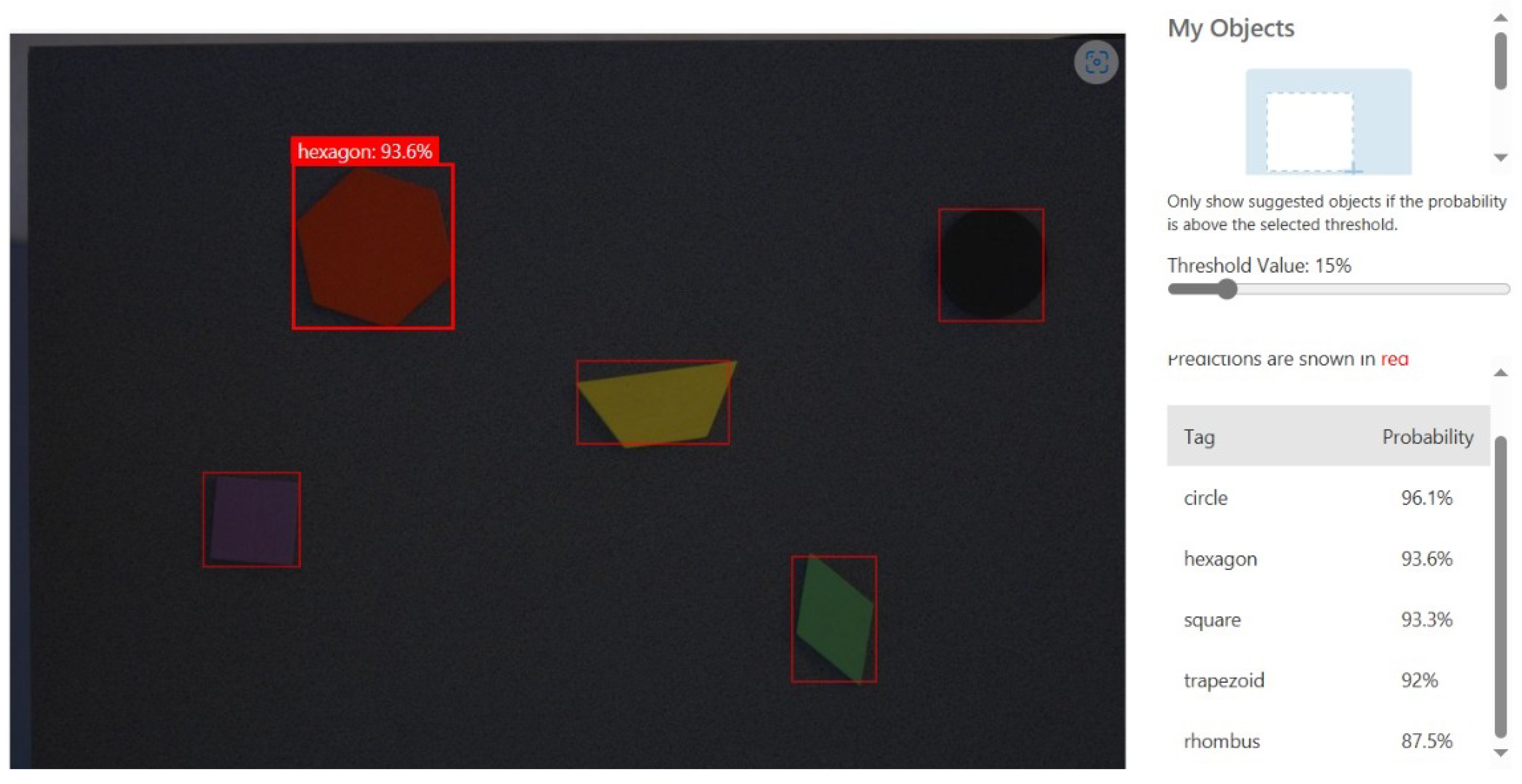
Figure 2.
Cloud Vision System Architecture.
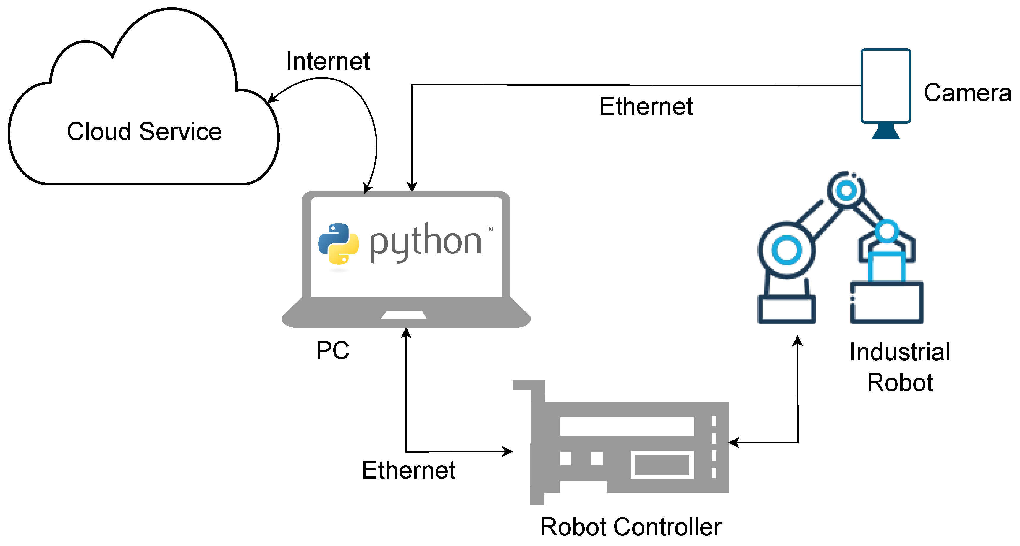
Figure 3.
(a) The physical system and its components. (b) The transform from the Robot Plane to the Vision Plane.
Figure 3.
(a) The physical system and its components. (b) The transform from the Robot Plane to the Vision Plane.
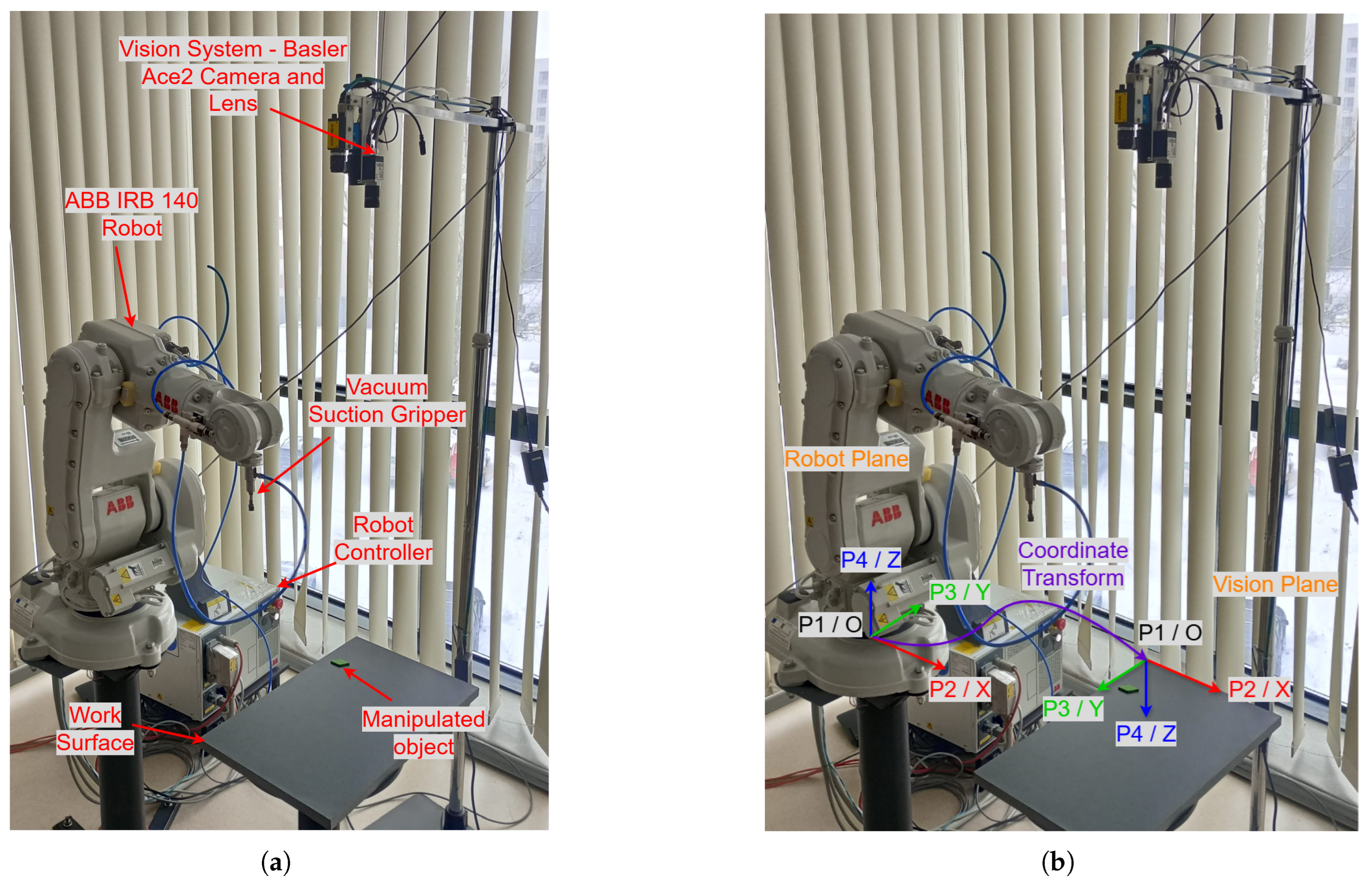
Figure 4.
The event diagram.
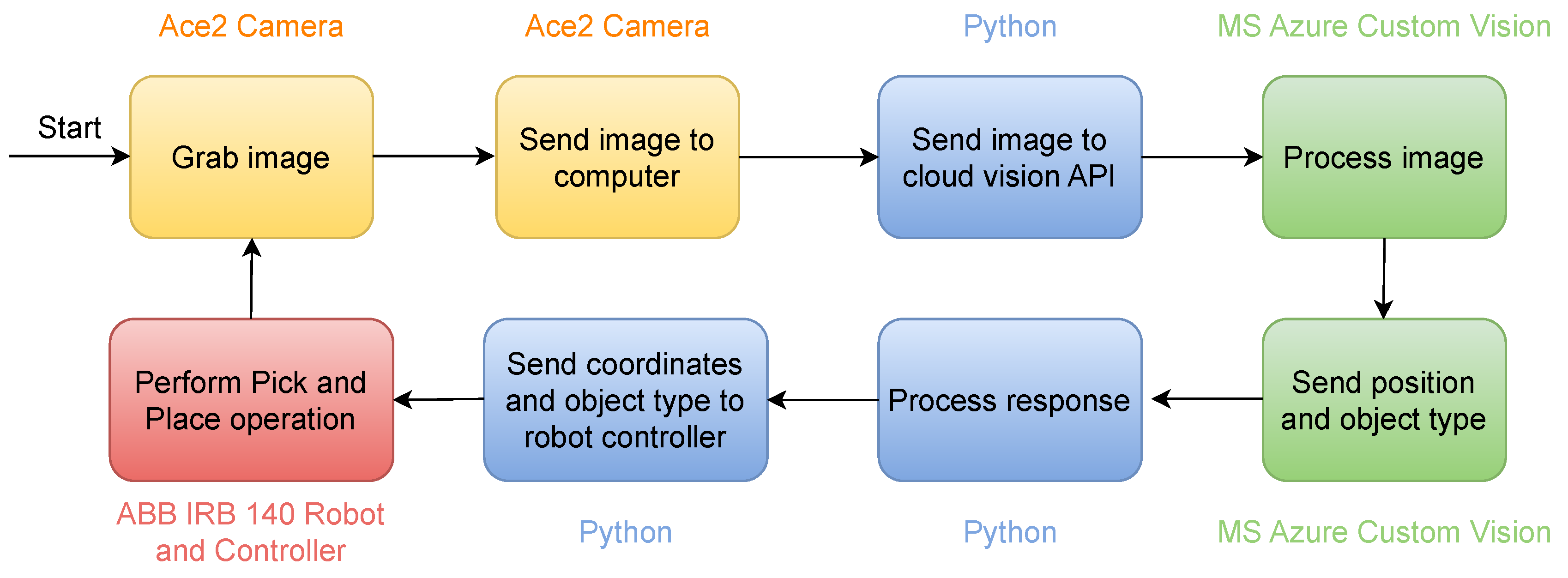
Figure 5.
Transforming from camera coordinates to workobject coordinates.
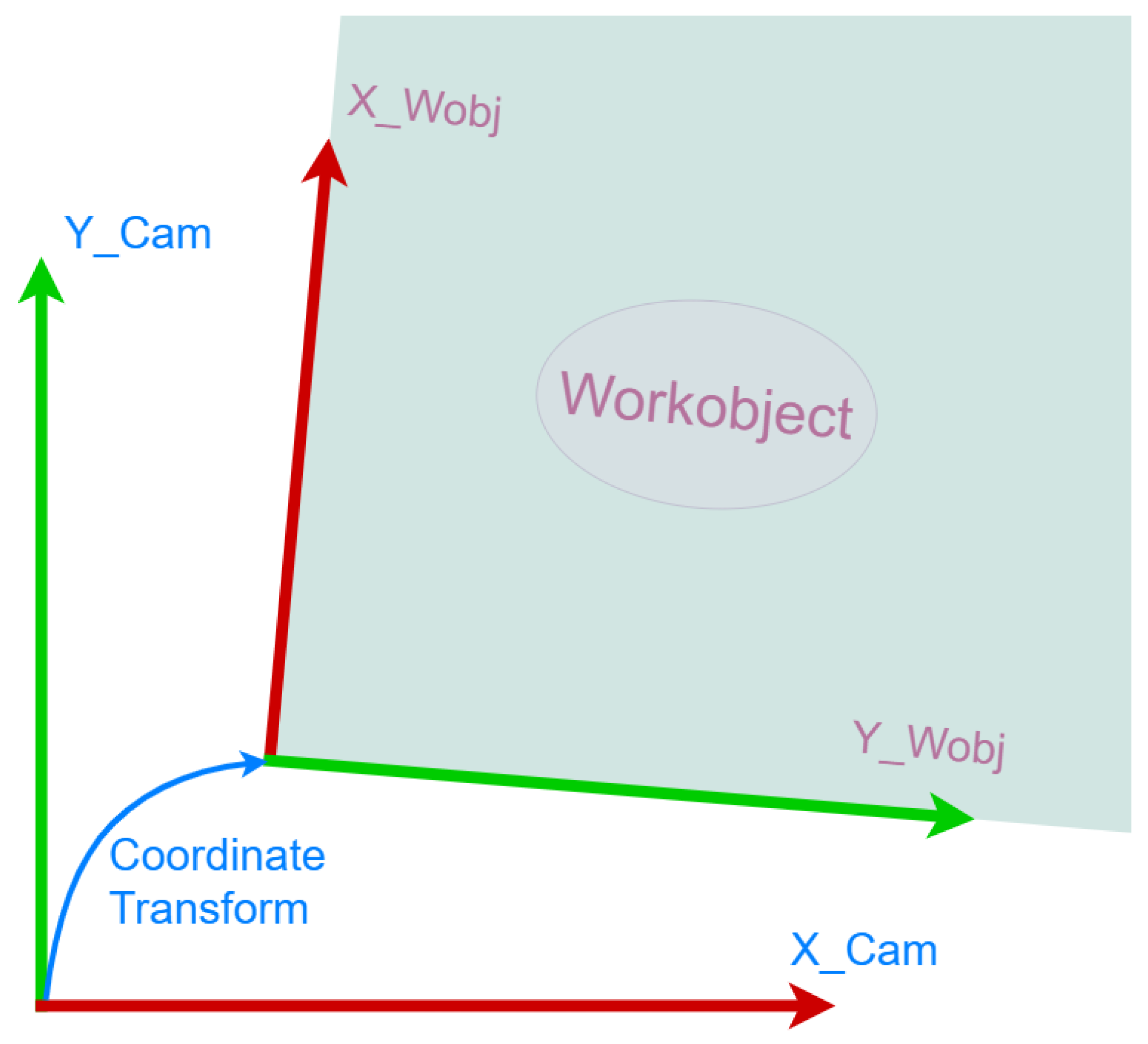
Figure 6.
(a) Image taken of the hexagonal object under natural light. (b) Image taken of the hexagonal object under artificial light.
Figure 6.
(a) Image taken of the hexagonal object under natural light. (b) Image taken of the hexagonal object under artificial light.
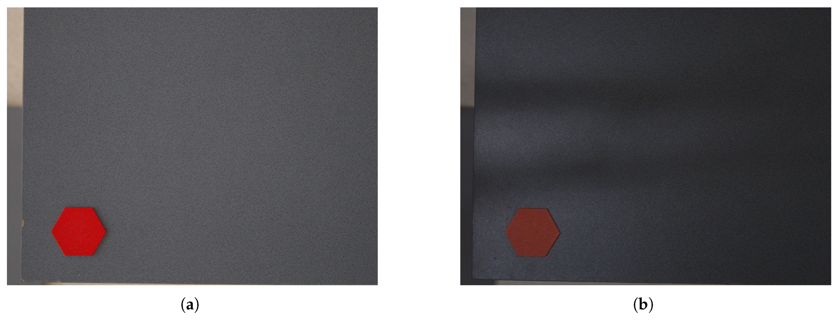
Figure 7.
The picking point, calculated as the center of the bounding box.
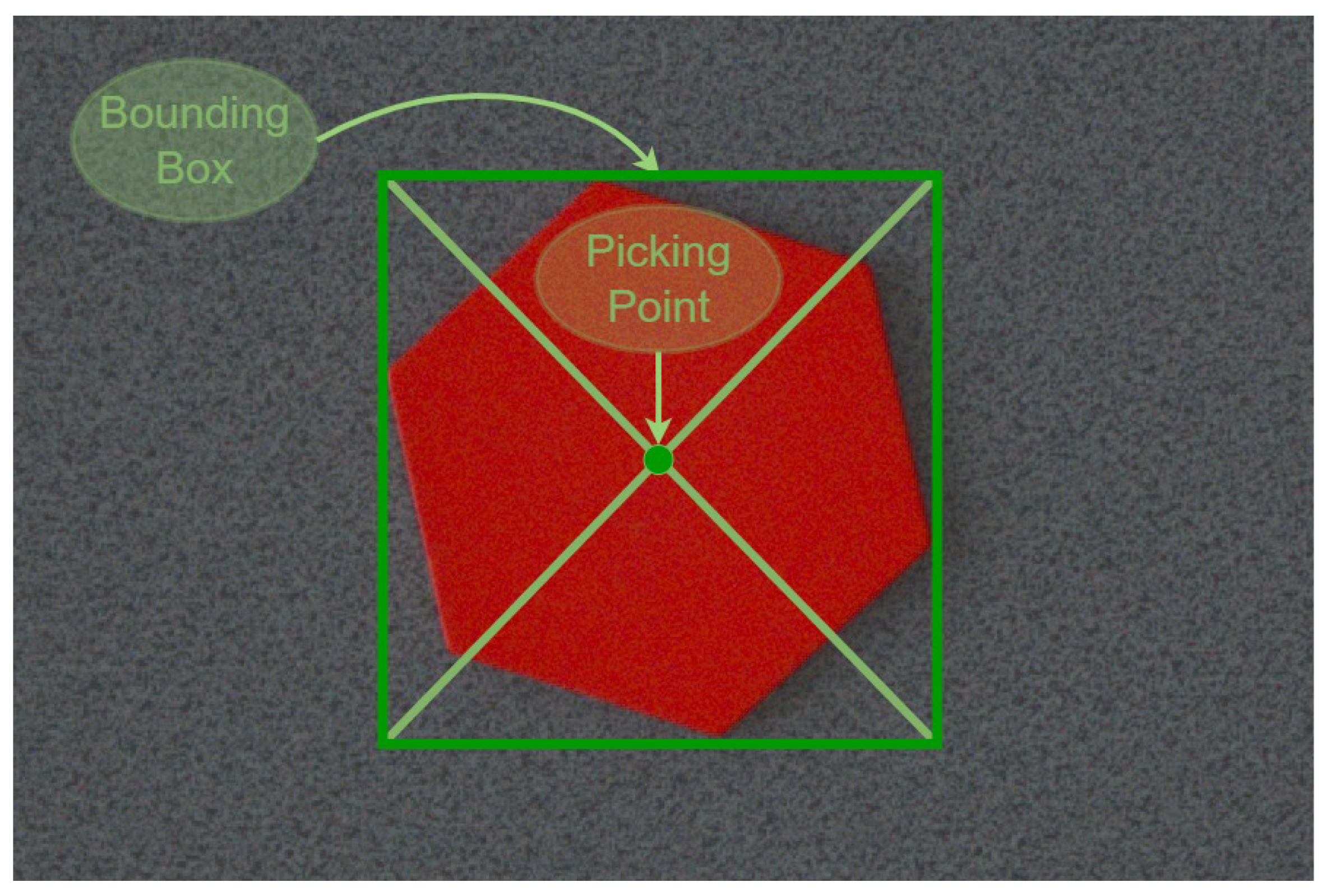
Figure 17.
Detection of dirty objects.

Figure 18.
Detection of overlapping objects.
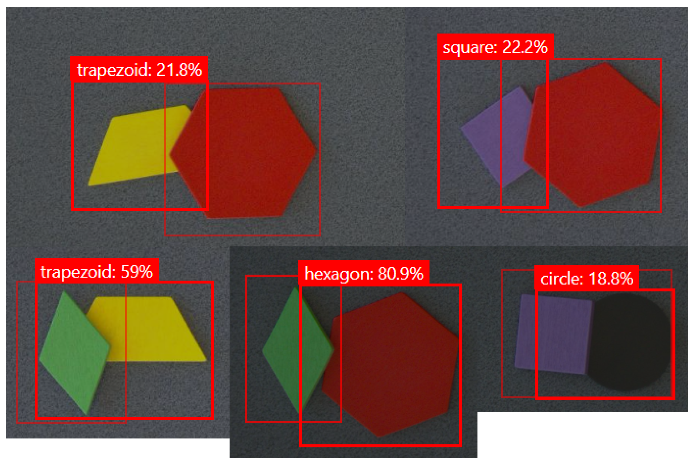
Figure 19.
(a) Confidence histogram for natural light after retrain. (b) Confidence histogram for artificial light after retrain.
Figure 19.
(a) Confidence histogram for natural light after retrain. (b) Confidence histogram for artificial light after retrain.
Disclaimer/Publisher’s Note: The statements, opinions and data contained in all publications are solely those of the individual author(s) and contributor(s) and not of MDPI and/or the editor(s). MDPI and/or the editor(s) disclaim responsibility for any injury to people or property resulting from any ideas, methods, instructions or products referred to in the content. |
© 2025 by the authors. Licensee MDPI, Basel, Switzerland. This article is an open access article distributed under the terms and conditions of the Creative Commons Attribution (CC BY) license (http://creativecommons.org/licenses/by/4.0/).
Copyright: This open access article is published under a Creative Commons CC BY 4.0 license, which permit the free download, distribution, and reuse, provided that the author and preprint are cited in any reuse.


