Submitted:
01 April 2025
Posted:
01 April 2025
You are already at the latest version
Abstract
Abstract Rail fasteners secure rail tracks to sleepers to prevent displacement, which makes them critical for railway safety. Regular track inspection is essential as long-term usage leads to fastener defects and track irregularities that require accurate measurement of geometric parameters of fasteners for proper maintenance. This paper proposes a method for fastener defect detection and geometric parameter measurement based on 3D linear laser sensor. Firstly, a 3D imaging system is constructed based on a 3D linear laser sensor to generate RGB-P bimodal data, which includes an RGB depth image and its corresponding point cloud. Secondly, the visual defect is detected and fastener area is located from the RGB depth image of railway track. By mapping the fastener area of RGB depth image to point cloud, the fasteners point clouds are rapidly segmented from railway track point cloud. Lastly, the PointNet++ network segments the fastener point cloud into individual components. Based on the spatial structure of fastener components, the specifications of insulated blocks, thickness of height adjustment pads, and bolt heights are measured. Experimental validation shows 100% precision and recall in visual defect detection. For fastener components with minimum specification differences of 1 mm, the measurement error remains below 0.5 mm. The system achieves a real-time detection and measurement speed of 4.32 km/h, effectively replacing manual inspection for high-speed railway fasteners.
Keywords:
Three-dimensional linear laser sensor
; Railway fastener
; Defect detection
; Geometric parameters measurement
; YOLOv8 network
; PointNet++ network
1. Introduction
Railway fasteners are essential elements within railway infrastructure, designed to secure the rail to the sleeper, thereby preventing rail misalignment and ensuring adherence to standard gauge specifications. In alignment with China’s railway track design criteria, the predominant fastener types utilized in high-speed railway systems include “Vossloh-300,” “WJ-7,”and “WJ-8,” as depicted in Figure 1. These fasteners, characterized by their „ω” configuration, are commonly designated as „ω-shaped” clips. Generally, these fasteners comprise a track bolt, an „ω-shaped” clip, an insulated block, height adjustment pads, and various other components illustrated in Figure 2, with minor compositional differences among the distinct clip types[1].
Prolonged utilization of fasteners may result in a range of defects, which can be classified into visual defects (including bolt missing, fracture, and clip skewed) and structural defects (such as excessively loose or tight fasteners), as illustrated in Figure 3. The visual defects have different textures, while the structural defects are only reflected in the height differences, and their appearance is exactly the same as that of the normal fasteners. These defects can impact ride quality and may even lead to train derailments, thereby presenting considerable safety risks to railway operations. In addition to regular inspection of fastener defects, The rail track of high-speed railway need to be adjusted accurately to ensure the high demands of track regularity[2,3] . During the adjustment of the track, the insulated block and the height adjustment pad may be replaced by those of different thicknesses according to the track adjustment plan [4,5,6]. Therefore, accurate detection of fastener defects and measurement of geometric parameters are both essential for railway maintenance. Currently, Fastener defects can be detected automatically by installing sensors on the rail inspection vehicle, while the geometric parameters of the fastener system are measured manually, a method that is time-consuming and prone to errors. Consequently, there is an urgent requirement for an automated and efficient system for defect detection and measurement of geometric parameters in high-speed railway fasteners.
2. Related Work
Current investigations into the measurement of fastener geometric parameters are limited; however, researchers have extensively explored fastener detection, categorizing the methodologies primarily into two types: those utilizing Two dimension(2D) vision and those employing three dimension(3D) vision techniques. Detection methods based on 2D vision imaging involve rapidly capturing 2D images of the railway with 2D cameras, and then using target localization, feature extraction, and and track image classification[7]. Typically, methods such as template matching[8], edge segmentation[9], and gray level statistics[10] are used to quickly locate the fastener from the 2D track image. Subsequently, different features of the fastener image are extracted based on prior knowledge and the shape of the fastener, such as Histogram of Oriented Gradients (HOG) features[11], local binary features[12], orientation fields[13], bag of words features[9], and semantic features[14]. Finally, classifiers are used to categorize the features and identify fasteners with visual defects. These methods are highly dependent on specific scenes and lack robustness to environmental changes. In recent years, Deep Convolutional Neural Networks (DCNN) have achieved groundbreaking success in the field of image classification. DCNNs have multi-layered end-to-end networks that can directly extract features and classify targets. Networks such as AlexNet CNN, R-CNN, Mask R-CNN, Fast R-CNN, ResNet, and the Yolo series have yielded good detection results in fastener defect detection applications[2,3,15]. By constructing samples with normal and visual defective fastener images to train the DCNN model, the model can directly output detection results, demonstrating good robustness to the environment. The above-mentioned 2D vision imaging methods can detect fasteners with visual defects and have been successfully used for rapid detecting visual defects. However, 2D vision imaging can only obtain 2D images of the track, and thus cannot detect fastener tightness defects or measure the geometric parameters of the fastener.
In recent years, 3D vision imaging technology has gradually been used for track detection, utilizing RGB-D depth cameras or linear structured light cameras to obtain both 2D images and 3D depth images of the scene. By processing 3D depth data or fusing 2D images with 3D depth information, various defects of fasteners can be detected. Shi[4] used an RGB-D sensor to obtain RGB images and depth images (Depth, D) of subway tracks, referred to as RGB-D images. By fusing depth images with RGB images, the influence of environmental light on detection results is overcome, thereby improving the accuracy of visual defect detection. Nevertheless, RGB-D cameras exhibit limited accuracy in depth measurement, rendering them unsuitable for precise geometric parameter measurement. Structured light imaging can accurately obtain 3D data of the scene. Jin et al.[16] used a 3D Ranger camera to obtain railway intensity (Intensity, I) and D images, forming a bimodal I-D image. They located fasteners in the depth image and fused the location parameters with the intensity map to achieve precise fastener location, and constructed a ResNet network to detect visual defects from the intensity image. Similarly, Zhan et al.[17] used the height of fasteners in the depth image to quickly locate the fastener and constructed a RailNet DCNN modal to extract features and classify the intensity image of fasteners, thereby detecting visual defects. The above 3D vision imaging methods can simultaneously obtain color and depth information of the scene. By fusing the color and depth data of bimodal images, the influence of environment can be effectively overcome, improving the accuracy of detection of visual defects of fasteners. However, these methods have not been studied for the detection of fastener tightness defects and measurement of the geometric parameters of fasteners.
To detect fastener tightness defects, Han et al.[18] used a 3D Ranger camera to obtain 2D depth images and 3D point clouds of the track. Based on the template matching algorithm, they quickly located fasteners in the depth image and used the watershed algorithm to segment the bolt of the fastener in the depth map. The structural defects of fasteners were detected based on the height difference between the bolt height and the rail edge. Gao et al.[19] used line structured light sensor to obtain 3D point clouds of track fasteners. They segmented the 3D point clouds of fastener bolt using prior knowledge and regional growth methods and detected severely loose fasteners based on bolt height. Wang et al.[20] used a 3D camera to obtain sparse 3D point cloud data of the track, constructed an accumulated height function, and segmented the rail and fastener based on prior knowledge. They detected fastener tightness by calculating the height difference between the bolt and the non-wearing area outside the rail head. This method can accurately detect severely loose fasteners. Mao et al.[21,22] used the structured light sensors to collect the railway point cloud, and detect visual defects based on decision trees according to the bolt height, and the tightness of the fastener was judged by calculating the gap of the clip according to the spatial position of the centerline. The above 3D measurement methods can detect the over-loose fasteners, but they do not conduct research on the measurement of fastener geometric parameters. In order to measure the geometric parameters, Cui et al.[23] used a structured light camera to build a 3D measurement system to collect dense point cloud of the track. They measured the rail gauge, bolt height, height adjustment pads based on dense point clouds. However, this method has not considered the defect of the fastener.
In summary, 2D vision imaging methods can rapidly detect visual defects of fasteners, and 3D vision sensors can simultaneously obtain color and depth images of the scene. By combining multi-modal data, the influence of environment and lighting can be further overcome, enhancing the accuracy of visual defect detection. 3D imaging can accurately obtain 3D point clouds of the track, and by utilizing the 3D spatial structure of fasteners, the tightness defects of fasteners can be detect. However, most of the research mainly focuses on defect detection, with relatively little research on the measurement of fastener geometric parameters. Moreover, there is a lack of a detection technology that can simultaneously detect fastener defects and measure the geometric parameters of fasteners. Therefore, this paper proposes a method for detecting defects and measuring the geometric parameters of fasteners based on 3D linear laser sensor.
The workflow of our method is illustrated in Figure 4. Initially, a 3D imaging system is constructed based on a 3D linear laser sensor to generate RGB-P bimodal data, which includes an RGB depth image and its corresponding point cloud. Subsequently, the visually defective fasteners is detected and visually normal fasteners is located from the RGB depth image using the Yolov8s network. The point clouds of visually normal fasteners are then rapidly segmented based on the RGB-P bimodal data mapping. Finally, the point clouds of fastener components are segmented using the PointNet++ network, and the geometric parameters of the fastener components are measured based on their spatial structure. The main contributions of this research are summarized as follows:
(1)The RGB-P bimodal data, including the RGB depth image and corresponding point cloud, is constructed based on the 3D linear laser sensor to facilitate the detection of defects and the measurement of geometric parameters of railway fasteners. The visual defect of fastener is rapidly detected from the RGB image, and the geometric parameters are accurately calculated by processing the fastener point cloud based on the spatial structure of fastener components.
(2)The geometric parameters of railway fasteners, including the specifications of insulated blocks and the thickness of height adjustment pads, are accurately quantified for precise railway fine-tuning. For fastener components with minimum specification differences of 1 mm, the measurement error remains below 0.5 mm.
(3)The 3D measurement system of railway fastener is constructed based on the 3D linear laser sensor to detect defects and measure the geometric parameters of fastener, the system achieves a real-time detection and measurement speed of 4.32 km/h, effectively replacing manual inspection for high-speed railway fasteners.
The remainder of this paper is organized as follows: Our method is detailed in Section Ⅲ, while Section Ⅳ verifies the precision through a full experimental demonstration of the defect detection and geometric parameter measurement. and finally, conclusions are summarized in Section V.
3.1. The 3D Imaging System Construction Based on 3D Linear Laser Sensor
3.1.1. Data Acquisition with 3D Linear Laser Sensor
Constructing an effective imaging system is crucial for efficient and precise railway fastener inspection. This research utilizes Gocator 2450 3D linear laser sensor, produced by LMI, to collect track data. The sensor employs a blue light laser with a 405nm wavelength, offering a depth of field of 550mm and a field of view that spans from 145mm to 425mm. It boasts a linear measurement accuracy of 0.01mm in the z-direction. The measurement accuracy provided by the sensor ranges from 0.019mm to 0.06mm and decreases progressively from close range to far range. It can operate at a maximum acquisition frequency of 5000Hz, capturing up to 5000 lines of profiles per second.
The sensor is mounted vertically on the inspection vehicle, allowing it to scan objects within its depth and width field of view. Configuring the sensor for external trigger mode and trigger distance, the user can set parameters such as field of view, height range, and horizontal spacing. Each trigger pulse from an external source prompts the sensor to scan a line profile. An encoder attached to the inspection vehicle’s wheels generates pulses that correspond to wheel rotations, serving as input for the sensor to regulate profile acquisition. When the inspection vehicle’s speed is lower than the sensor’s maximum acquisition speed, the sensor scans the track profile heights within the field of view autonomously, synchronizing its scanning speed with the vehicle’s speed. The principles and schematic diagram of railway fastener point cloud data collection are illustrated in Figure 5.
Detecting defect of fastener based on point clouds processing can be a time-intensive process. To enhance computational efficiency, we construct RGB-P bimodal data, which integrates an RGB depth image with its associated point cloud. Each pixel in the RGB depth image corresponds to a specific point within the point cloud representation. The RGB depth image conveys the fastener’s shape and existence, whereas the point cloud offers spatial configuration and depth details. This methodology facilitates the detection of visual defects in the fastener and its localization via the RGB depth image, while the geometric parameters of the fastener can be derived from the point cloud data.
For the construction of RGB-P bimodal data, a coordinate system is established for data acquisition, tailored to the characteristics of the 3D laser sensor. The Y-axis aligns with the direction of the rail, the X-axis is perpendicular to the rail, and the z-axis represents vertical height. The laser sensor’s sample interval in the X and Y directions is denoted as dx and dy, with dy also acting as the trigger distance. The dimensions of the scanned area are defined by the width (W) and length (L), and the number of points along the X and Y axes is represented by M and N, respectively. These values are derived from the equations M=W/dx and N=L/dy, with the parameters W, L, dx, and dy user-defined for the 3D laser sensor. N and M correspond to the rows and columns of the point clouds and the RGB depth image.
If the depth image is represented by a grayscale image, then each pixel corresponds to a height. However, grayscale images only have 256 gray levels, which limits the amount of information they can contain. In contrast, RGB image can depict 224 colors, and each height segment is represented by RGB color. This enables the representation of over 160 million height segments. As a result, this paper constructs RGB depth image to correspond one-to-one with the point clouds. This indicates that the corresponding pixel in the depth image appears in the same position as the point cloud map.
Each row in the profile contains M points, and a point cloud data set is formed by N rows of these profiles. This specific point cloud data set corresponds to an image with a size of N×M. A point located at the i-th row and j-th column within this set of point clouds can be represented as (Xi, Yj, Zij), where i=1,2,...,N, j=1,2,...,M. The depth field of the sensor is H, which equals Zmax-Zmin, where Zmax and Zmin are the maximum and minimum measurement heights of the 3D laser sensor, respectively, and . The height H is divided into Num parts as equal interval , where and is set by users. A color table is then established, and Num+1 different colors are selected in the color table. This enables the representation of different height ranges with different colors, and the relationship between height and color can be expressed as follows.
where [x] represents an integer for x, ni is the index of color table.
Due to the impact of the 3D line laser imaging technique and track conditions, local occlusions occur, creating blind spots when the 3D laser scans the railway track. As a result, the height value of the blind area becomes invalid. Thus, it is essential to verify the validity of the height value for each point when constructing the depth image. In summary, the algorithm for constructing RGB depth image is outlined as follows:
Step 1: Getting the parameters of the sensor, including dx, dy, L, W.
Step 2: Constructing an empty RGB image I with a size of .
Step 3: During 3D laser sensor scanning of the railway, it is necessary to determine whether the Zij value of point cloud Pij(Xi, Yj, Zij) is valid. If Zij is a valid value, the point Pij is then mapped into a 2D image I with coordinates (i, j), and its color is determined by Equation (1).
Step 4: If Zij of point Pij(Xi, Yj, Zij) is an invalid value, the pixel of the image at coordinates(i, j) is represented by the last color in the color table.
Step 5: Save RGB depth images along with point cloud with the same filename, and output RGB-P bimodal data of the scanned scene, as shown in Figure 6.
3.1.3. The Mapping Relationship of RGB-P Bimodal Data
In this research, the collected railway profiles are consolidated into a point cloud and recorded in a text file. Each line within this file contains three numerical values that represent the X, Y, and Z coordinates of a single point. Given that the size of the RGB depth image is M×N, the text file contains M×N lines, each representing a point. The point clouds are then imported from the text file into a container of point structures, referred to as Vect. The number of points in the Vect container corresponds to the pixel count of the RGB image, with each point detailing the x, y, and z coordinates of the point cloud. Given image I and its coordinates (i, j), the mapping relationship between image I and point cloud Pid(Xi, Yj, Zij) in Vect is described by Equation (2):
Any pixel in the image can be located with the corresponding point cloud using formula (2).
3.2. Visual Defect Detection and Fastener Region Location
Fasteners’ visual defects are manifested as conspicuous texture deviations compared to their normal states, while structural defects are predominantly reflected in height disparities. The linear laser sensor operates on the triangulation principle for imaging, and the resulting RGB depth image remains unaffected by illumination conditions. Additionally, the „ω-shaped” fastener features a relatively simple geometry. For normal fasteners of the same type in appearance, the texture of the RGB depth images of their tracks is nearly identical. In contrast, defective fasteners exhibit substantial shape differences from normal ones. As a result, conventional deep-learning-based object detection algorithms can efficiently identify fastener defects from RGB depth images. Common deep-learning object detection methods encompass the R-CNN series[24], the SSD network[25], and the Yolo series[26], among others. These object detection networks have found extensive applications across diverse fields, each boasting its own set of advantages. In this study, the classic Yolov8 network is employed to detect fastener defects in RGB depth images[27]. The use of rectangular bounding box detection enables rapid localization of fasteners. Leveraging the positions of the rectangular bounding boxes of objects and the mapping relationship between images and point clouds, the point cloud of the visually normal fastener region can be swiftly segmented.
Given the varying nature of visual defects of fasteners and the similar appearance of normal fasteners and those with structural defects, this paper categorizes visual defects as „defect”. Fasteners that appear visually normal and structural defects, are labeled as „normal”. To facilitate the simultaneous detection of defective fasteners and the precise segmentation of the fastener regions, the rectangular labels for normal samples are designed to closely match the minimum bounding rectangle around each fastener.
We compiled a training dataset for the Yolov8s model using RGB depth images of „ω-shaped” fasteners. The trained model generates a prediction box for each detection result, represented by (x, y, w, h). Here, (x, y) indicates the top-left corner of the rectangle, and w and h denote the width and height of the box, respectively. Therefore, we utilized the box (x, y, w, h) to locate the visually normal fastener area from the railway image.
The Point clouds of visually normal fastener area can be rapidly segmented based on the relationship of RGB-P bimodal data with Equation (1). The detection results of fastener based on the YOLOv8s is shown in Figure 7 and the flowchart and result of point clouds segmentation of fastener is presented in Figure 8.
Given that geometric parameters cannot be directly calculated from 2D images, point cloud analysis is employed to determine the geometric parameters of fasteners. Precise measurement of fastener geometric parameters requires segmentation of point cloud data into individual fastener components. The geometric parameters of these components can then be computed by analyzing their spatial interrelationships and relative positions.
3.3.1. Fastener Component Point Cloud Segmentation Using PointNet++ Network
Point cloud segmentation methodologies can be broadly categorized into traditional approaches (region growing, clustering, RANSAC plane segmentation) and deep learning-based methods[28]. Region growing algorithms initiate from a seed point and iteratively incorporate adjacent points meeting predefined criteria until convergence[29]. However, this approach is highly sensitive to initial parameter selection, particularly seed point placement, which can significantly impact segmentation outcomes. While clustering algorithms (e.g., K-means and DBSCAN) are extensively employed, their effectiveness is constrained by parameter sensitivity, including cluster quantity specification and density threshold determination[30]. RANSAC-based plane segmentation employs random sample consensus to identify optimal plane models and delineate planar regions[31]. While this approach excels in environments dominated by planar surfaces (e.g., indoor scenes), it proves inadequate for complex geometric structures. In contrast, deep learning approaches leverage neural networks to perform point cloud segmentation, with architectures such as PointNet and PointNet++ demonstrating remarkable capability in handling complex geometric structures. PointNet++ overcomes these limitations by its unique hierarchical feature learning framework. It can better capture local geometric structures at multiple scales, making it more suitable for segmenting the complex point clouds of fasteners. Given its hierarchical architecture and enhanced segmentation capabilities, PointNet++ was used for the primary methodology for fastener component point cloud segmentation in this study.
PointNet++, introduced by Qi et al.[32], represents a significant advancement in 3D point cloud processing architecture. This framework has demonstrated exceptional versatility across various applications, including point cloud classification, semantic segmentation and 3D object recognition. The architecture, illustrated in Figure 9, implements hierarchical feature learning through a set abstraction operation that processes local point cloud regions at multiple scales. The PointNet++ architecture processes point cloud data as input. This network is characterized by a hierarchical feature learning encoder and a task-specific prediction layer, which facilitates either classification or segmentation. The hierarchical feature learning process comprises two key operations: sampling and grouping, and local feature learning using PointNet layers. The sampling and grouping process utilizes farthest point sampling to identify representative key points. To address point cloud sparsity and irregularity, multi-scale grouping or multi-resolution grouping is implemented, which constructs spherical neighborhoods with different radii around each sampled point to handle varying point densities. In the feature extraction phase, the PointNet architecture processes the sampled groups to extract comprehensive local-to-global features. This hierarchical feature aggregation mechanism captures both point-wise characteristics and contextual information within local neighborhoods, enabling effective representation of geometric relationships. For classification tasks, the PointNet++ network typically employs categorical cross-entropy as the loss function, while for segmentation tasks, it uses point-wise cross-entropy, defined as:
where is the number of samples, C is the number of categories,is the probability of the true label category (0 or 1), and is the category probability output by the network.
The network was optimized using the Adam optimizer, which employs adaptive moment estimation to dynamically adjust learning rate, facilitating faster convergence and enhanced model performance. The network training hyper-parameters are detailed in Table 1. The trained PointNet++ model enables precise segmentation of fastener components, yielding individual point cloud subsets for each component. These segmented point clouds serve as the foundation for subsequent geometric parameter extraction and analysis.
3.3.2. Geometric Parameters Calculation of Fastener
The „ω-shaped” fastener is primarily composed of bolt, metal clip, insulated block, height adjustment pads under the rail, height adjustment pad under the iron plate, and various other components. Among these components, the bolt presses the metal clip to secure the rail on the sleeper, hence the height of the bolt upper surface reflects the tightness of the fastener. The insulated block is used for fine adjustment of the rail gauge, while the height adjustment pad under the rail and under the iron plate are used for adjusting the rail height. These two types of pads come in different specifications.
Track maintenance operations frequently require precise adjustments of critical parameters, particularly vertical alignment and gauge spacing between parallel rails. These precise geometric adjustments are fundamental to ensuring safe and comfortable high-speed rail operations, contributing significantly to China’s exemplary high-speed railway performance.
During operational service, track geometry gradually deteriorates due to dynamic loading and environmental factors, necessitating periodic adjustments to maintain optimal gauge and vertical alignment parameters. Long-term operation leads to variations in fastening system component geometries. Accurate measurement of these parameters is crucial for maintenance planning and component selection during track adjustment procedures. Traditional manual measurement methods are both time-intensive and prone to human error.
This study demonstrates the point cloud-based geometric parameter measurement methodology using the WJ-8 fastening system as a case study. The proposed methodology is generalizable to other fastener systems, including the Vossloh-300 series and WJ-8. Figure 10 presents the structural schematic, in-situ photograph, and point cloud representation of the WJ-8 fastening system.
(1) The specification of insulated block. Insulated blocks are manufactured in five standard specifications (designated as No. 7 through No. 11), with corresponding nominal thicknesses ranging from 7 mm to 11 mm in 1 mm increments. Track gauge adjustment can be achieved through the selective replacement of insulated block, where the appropriate thickness is chosen to achieve the desired gauge modification. Figure 11 illustrates the installation configuration and structural details of the insulated blocks, where d denotes the block thickness. Given that the insulated block’s inner surface interfaces directly with the rail edge , its thickness can be computed as the differential between the x-coordinates of the insulated block’s outer edge and the adjacent rail edge. The insulated block thickness d can be determined using the following mathematical expression:.
In equation (3) and are x-coordinates of the outer edge of the insulated block and the adjacent edge of the rail, respectively. To accurately calculate and , this paper fits lines to the point clouds of the outer side of the insulated block and the edge of the rail obtained from PointNet++. The x-coordinates of these lines are correspond to the values of and .
(2) The height adjustment pads. The WJ-8 type fastener is suitable for ballastless tracks and comes with two types of height adjustment pad: the height adjustment pad under the rail and the height adjustment pad under the iron plate. The height adjustment pad under the rail is installed beneath the rubber pad and above the iron pad, and is available in four thickness specifications: 1 mm, 2 mm, 5 mm, and 8 mm. The height pad under the iron plate is installed beneath the iron plate and above the insulation buffer pad, and is available in two thickness specifications: 10 mm and 20 mm. According to the high-speed railway maintenance standards, when the rail elevation is less than or equal to 10 mm, only the height pad under the rail needs to be installed; when it exceeds 10 mm, the height adjustment pad under the iron plate will be installed. A single set of fastener systems can accommodate a maximum of two track-level fine-tuning pads, with a total thickness not exceeding 10 mm. These two types of height adjustment pad can raise the rail by a maximum of 30 mm.
A 3D imaging system composed of 3D linear lasers can scan a portion of the point cloud on the upper surface of the rubber pad. Therefore, the thickness of the height adjustment pad under the rail can be directly measured based on the height of the upper surface of the rubber pad, the height of the upper surface of the iron pad, and the thickness of the rubber pad.
The thickness of the height pad under the iron plate can be calculated with formulation
In the equation (4), is the height of upper surface of rubber pad, which has been marked as ⑥. is the height of upper surface of iron plate, which has been marked as ④. is the thickness of rubber pad (for the WJ-8 type fastener, this value is 10mm typically).
The thickness of height pad under the iron plate can be calculated using formula
In the equation (5), represents the height of the upper surface of the iron plate limit pillar, which has been marked with the red rectangle. represent the height of upper surface of the sleeper support, which has been marked as ⑧. represents the thickness of the butter pad beneath the iron plate and represents the height difference between the upper surface of the iron plate limit pillar and the middle-upper surface of the iron plate (is 38.2mm typically for the WJ-8 type fastener).
Bolt Height Analysis for structural defect detection. Fastening system deficiencies, including both under- and over-torqued conditions, cannot be reliably detected through conventional 2D image analysis. Fastener can be compromised through multiple mechanisms: cyclic loading from train-induced vibrations, environmental factors such as moisture infiltration and subsequent freeze-thaw cycles in bolt holes, which generate substantial longitudinal forces accelerating bolt loosening. Compromised bolt torque leads to reduced clamping force, potentially compromising rail restraint and threatening operational safety. Conversely, excessive torque application can result in over-stressed clips, potentially leading to fatigue failure under dynamic loading conditions. Regular monitoring of bolt torque conditions is therefore critical for maintaining system integrity. Deviations in bolt height relative to the base-plate surface serve as a quantitative indicator of improper torque conditions. This geometric parameter enables objective detection of fastener structural defects, facilitating detection of both under- and over-torqued conditions. The bolt height parameter () can be determined by
Where represents the upper surface of bolt, which has been marked as ①.
The value of represents the looseness of the fastener. If is higher than a threshold value, the fastener is considered loose; conversely, if is lower than a threshold value, the fastener is considered over-tight.
4. Experimental Results and Analysis
This section presents experimental validations to evaluate the effectiveness of the proposed methodology through five aspects: measurement accuracy assessment of the 3D imaging system, accuracy analysis of visual defect detection, validation of the PointNet++ network’s segmentation capabilities, verification of geometric parameter measurement accuracy, and time analysis of the detection and measurement process. The experiments were conducted on both experimental rail tracks and operational railways near Nanchang, China, due to the unavailability of public railway datasets for fastener detection validation. The algorithm developed in this study was implemented in Python and executed on a computational system with the following specifications: CPU: i7-13700kf (3.6GHz), RAM: 64GB, GPU: 4070ti (12GB), and OS: Windows 11 (64-bit).
4.1. Evaluation of the Measurement Accuracy of the 3D Imaging System
The precision and reliability of the 3D imaging system are fundamental prerequisites for accurate defect detection and geometric parameter measurement. System accuracy was validated using a calibrated standard block (shown in Figure 12(a)) as a reference standard. The reference gauge block features precisely machined steps with height differentials of 6.000 mm and 11.500 mm (±0.020 mm manufacturing tolerance). The sensor’s trapezoidal field of view (FOV), illustrated in Figure 12(b), exhibits optimal measurement accuracy in the near-field region where the projection width is maximum. The sensor was mounted on a track inspection vehicle to maintain consistent positioning within the optimal measurement range during data acquisition. The resulting point cloud representation of the step gauge is presented in Figure 12(c). Height differential measurements were performed across six step transitions and compared against calibrated reference values, with results summarized in Figure 12(d). Experimental validation demonstrates measurement deviations within 0.019-0.054 mm of reference values, confirming system compliance with required precision specifications.
The precision (P) and recall (R), which are used to evaluate the accuracy of visual defect detection, are defined as follows:
where FP is the number of false positive result, and TP is the number of true positive results; FN is the number of false negative results.
The Intersection over Union (IoU) is employed to evaluate the accuracy of location region. IoU is defined as:
The range of IoU is [0,1], and a higher value indicates a more accurate result.
The defect detection and location of the fastener area are analyzed using a comprehensive dataset consisting of 5,800 railway RGB depth images. This dataset encompasses 4,000 samples of normal fasteners and 1,800 samples of visually defective fasteners. The dataset includes three types of fasteners: WJ-7, WJ-8, and WJ-2. Specifically, the WJ-7 and WJ-8 types of fasteners are sourced from ballastless tracks. The track environment of these ballastless tracks is relatively favorable, free from interference caused by crushed stones and debris. In contrast, the WJ-2 type of fasteners originates from ballasted tracks, where crushed stones and weeds are present on the tracks.The dataset was partitioned according to a ratio of 7:1.5:1.5 for the training, validation, and testing subsets, respectively.
The detection outcomes for both normal and defective fasteners are illustrated in Figure 13. Specifically, Figure 13(a)-(b) delineate the localization results for visually normal fasteners within the ballastless track imagery. Conversely, Figure 13(c)-(e) present the defect detection and localization results pertaining to ballasted tracks. Notably, Figure 13(c) depicts an excessively loose fastener, wherein the clip’s position within the image aligns with that of a normal fastener. Furthermore, the fastener presented in Figure 13(e) exhibits visual defects, characterized by a slight tilt in its clip. The proposed methodology accurately identifies this specific defect type.
The fastener detection result based on Yolov8s network is compared with other object detection method, such as Faster R-CNN, SSD and the latest Yolov11s network. The comparison for visual defect detection based on different methods is shown in Table 2. Since the RGB depth images of railway are not affected by ambient light, and the texture of the fastener images is relatively simple, all the object detection algorithms exhibit a relatively high accuracy in detecting fasteners. Among them, the accuracy of Yolov8s is slightly higher than that of other methods. The detection accuracy rate and recall rate for both normal fasteners and defective fasteners are 100%.
The precision of fastener geometry calculations is contingent upon the efficacy of fastener area localization. This investigation quantifies the accuracy of target detection and localization. Fastener localization accuracy is assessed via the IoU, computed between the detected bounding box and the ground truth. Figure 14 presents the IoU distribution for 600 visually normal fastener areas, with values ranging from 0.92 to 0.99, arranged in ascending order for clarity. These findings suggest that RGB depth images facilitate accurate detection of fastener defects and precise localization of fastener regions.
4.3. Performance Evaluation for Point Cloud Segmentation by PointNet++ Network
The segmentation of the components of fasteners is a crucial step for the precise measurement of components. Therefore, the segmentation accuracy is evaluated with IoU, which is defined in equation (8).
The PointNet++ network was trained utilizing point cloud data derived from WJ-8 type fasteners. The researchers allocated the dataset, which consisted of 566 fastener point clouds, in a ratio of 7:1.5:1.5 for training, validation, and testing, yielding 85 test samples. The architecture of PointNet++ facilitates flexible control over the output point cloud density. As the output quantity of point clouds from the PointNet++ network diminishes, the time necessary for the network to segment the fastener point clouds correspondingly decreases. In the computation of insulation block specifications, an increased point cloud density enhances measurement accuracy. Consequently, this paper forecasts outputs for all input point clouds, ensuring that the quantity of input point clouds aligns with the number of predicted point clouds. The processing speed of the point clouds can be regulated by adjusting the appropriate point spacing (dx and dy), thus achieving a balance between processing speed and accuracy requirements.
To ensure precise geometric parameter measurements, this study implements comprehensive component segmentation, encompassing both parameter-relevant components and other distinct elements that, while not directly involved in calculations, contribute to system completeness. While detailed analysis of all components is beyond the scope of this paper, we focus on eight primary component types, with representative segmentation results illustrated in Figure 15 and Figure 16. The experimental results demonstrate that the PointNet++ network achieved an IoU of 1 for most components, with only minor variations observed in rubber pad segmentation. These results validate the network’s capability to accurately segment complex fastener point clouds, thereby providing high-quality component-specific point cloud data for subsequent geometric parameter calculations.
4.4. Result Verification of the Geometric Parameters Measurement
To verify the accuracy of the geometric parameters measured using our method, we conducted a series of experiments comparing manual measurements with those obtained using our 3D imaging system. The geometric parameters of interest include the height of the fastener bolts, the specifications of the insulated blocks, the thickness of the height pad under the rail, and the height pad under the iron plate. Manual measurements were taken using calipers or gap gauges as the ground truth, and the error was defined as the difference between the measurement results obtained by our method and those obtained through manual measurement.
Manual measurement of fastener parameters is time-consuming, particularly when accurately measuring the height of the bolts. Therefore, in this experiment, we measured 63 WJ-8 type fasteners. After manual measurement, we used a 3D measurement system to scan the track and obtain RGB-P bimodal data. The YOLOv8s model was employed to quickly locate the fastener areas in the RGB depth images. Using formula (1), we mapped the image coordinates into a 3D point cloud, allowing us to rapidly segment the fastener point cloud from the railway point cloud. The fastener point cloud was then input into a trained PointNet++ network to segment the point clouds of the various fastener components. We utilized formulas (3) to (6) to calculate the specifications of the insulated block, the thickness of the height pad under the rail, and the height pad under the iron plate, as well as the height of the bolts.
Results of Height Adjustment Pad. The height adjustment pad under the iron plate can be either 10 mm or 20 mm in thickness. For the 63 fasteners used in our experiments, the height pad under the iron plate are all 10 mm thick. The measurement results are shown in Figure 17(a). Due to the potential unevenness of certain sleeper support, some measurement errors have exceeded 1mm. However, given that the height pad under the iron plate vary in specifications by 10mm, measurement errors within 5mm can still accurately determine their specifications. These results demonstrate that our method can accurately determine the thickness of the height pad under the iron plate.
Among the 63 fasteners, some have a height pad under the rail with a thickness of 5 mm, some have a thickness of 2 mm, and some have no height adjustment pads, i.e., the thickness of the height pad under the rail is 0 mm. According to the fastener installation standards, the height pad under the rail is installed between the rubber pad and the iron plate, with the thickness of the rubber pad being 10 mm. Since there is usually no gap between the rubber pad and the height pad under the rail, we manually measured the total thickness of the rubber pad and the height pad under the rail using a vernier caliper. The thickness of the height pad under the rail is the difference between the total thickness and the thickness of the rubber pad. The measurement results of our method, manual measurement, and the error between our method and the ground truth are shown in Figure 17(b). The results indicate that the measurement error is within the range of 0-0.25 mm. Although slight deformations occur due to manufacturing errors and the pressure exerted by the rail on the rubber pad and the height pad under the rail, the measurement error is less than 0.5 mm. Therefore, we can accurately determine the thickness by rounding the measurements. The measurement results meet the required standards.
Results of Insulated Block. The specifications of the insulated blocks are determined by measuring the distance between the edge of the rail and the outer side of the insulation block. The accuracy of this measurement is influenced by the sampling interval dx. A smaller dx results in a smaller horizontal spacing between points. The sensor used in this study has a minimum dx of 0.1 mm and a maximum dx of 0.56 mm. A larger dx increases the sensor’s scanning frequency, making the point cloud more sparse. To test the accuracy of insulated block measurements at different sampling intervals, we conducted experiments with dx values of 0.1 mm, 0.2 mm, 0.3 mm, 0.4mm,0.47 mm, and 0.5 mm. The 63 fasteners used in the test have three specifications of insulated blocks: 8 mm, 9 mm, and 10 mm. For clarity, the number of fasteners is sorted in ascending order based on the specifications of the insulated blocks. The measurement results and errors for different sampling intervals are shown in Figure 18. The results indicate that as dx increases, the measurement error also increases. When dx is set to 0.5 mm, the measurement error for most fasteners exceeds 0.5 mm. Since the specifications of the insulated blocks change in 1 mm increments, an error exceeding 0.5 mm makes it impossible to determine the actual specification. When dx is 0.47 mm, the measurement error is generally within 0.5 mm. Therefore, to balance measurement accuracy and speed, the sampling interval dx must be less than 0.5mm, and it is recommended that dx be less than 0.47mm.
Results of Bolt Height. Among the 63 fasteners used, there are three categories: over-tight fasteners, normal fasteners, and loose fasteners. The measurement results of the bolt heights for these three categories are shown in Figure 19. Due to manufacturing errors, the bolt heights of normal fasteners and over-tight fasteners are almost indistinguishable. However, the bolt height of loose fasteners is significantly higher than that of normal fasteners and over-tight fastener. Therefore, we can determined the reference height of the bolt by measuring a large number of fully torqued fasteners and calculating their average bolt height. Fasteners exhibiting bolt heights that surpass this reference can be classified as over-loose, thereby facilitating the efficient detection of loose fastener defects.
4.5. Time Analysis for Detection and Geometric Parameters Measurement
The time analysis was conducted on the inspection and parameter measurement of 63 fasteners. The data acquisition system was configured with a horizontal sampling interval (dx) of 0.47 mm with a maximum sensor line frequency of 1200 Hz, and trigger interval (dy) of 1.0 mm. The inspection vehicle collected RGB-P data at a speed of 1.2 m/s (4.32 km/h). However, it should be noted that increasing the trigger interval leads to sparser point clouds while enabling higher data collection speeds. The actual dimensions of the fastener area are approximately 90 mm × 200 mm. Due to data loss in the localized region, the average number of point clouds per individual fastener is 33,786 points.
The algorithm execution comprises three sequential phases: (1) RGB-P-based fastener detection and region location using YOLOv8, (2) component-level segmentation using the PointNet++ network, and (3) geometric parameter measurement and analysis. The total processing time for 63 fasteners was 20.79 seconds (s), with an average computation time of 0.33s per fastener, where the PointNet++ segmentation represented the most time-consuming phase at 0.31s per fastener. The time required for detecting the visual defects and location area of fasteners from the RGB depth images of the railway tracks is only 0.02s. The time needed for defect detection algorithm based on point cloud processing is much longer than that for image processing. Given the average inter-fastener distance of 0.63 meter(m) and total inspection distance of 39.69 m, the average processing speed achieved was 1.91 m/s. This processing speed exceeds the data acquisition speed (1.2m/s), enabling real-time defect detection and geometric parameter measurement when the 3D linear laser sensor is mounted on track inspection vehicles. For reference, manual measurement of 63 fasteners typically requires approximately 30 minutes.
5. Conclusion
Fasteners are critical components in railway infrastructure, with their defects posing significant threats to operational safety. The geometric parameters of fasteners provide essential reference data for track fine-tuning, directly impacting railway safety and passenger comfort. This paper proposes a novel method for fastener defect detection and geometric parameter measurement based on 3D linear laser sensor. A 3D linear laser sensor mounted on a track inspection vehicle constructs a measurement system that collects RGB-P bimodal data. The visual defect detection and fastener localization are conducted from RGB images, while RGB-P data mapping enables efficient fastener point cloud segmentation. The PointNet++ network then segments the fastener point cloud into individual components, facilitating geometric parameter calculation based on their spatial structure, including insulated block specifications, height adjustment pad thickness, and bolt heights.
Experimental results demonstrate that the precision and recall in fastener visual defect detection and fastener location. The PointNet++ network successfully segments fastener components with an IoU approaching 1. Geometric parameter measurements of 63 WJ-8 type fasteners show that the thickness of height pad under rail remains error within 0.25 mm, meeting 1mm specified requirements. The thickness of height adjustment pad under the iron plate maintains an error within 1.8 mm, well within the 5 mm tolerance. Measurement accuracy for insulated block specifications correlates with point cloud horizontal interval density, requiring intervals no greater than 0.47 mm to meet 1mm specified requirements. While bolt height measurements effectively detect loose fastener defects, over-tightening detection shows limited reliability due to surface oil contamination and manufacturing variations. The 3D measurement system developed in this research demonstrates capability for automated detection of both visual and loose fastener defects while providing rapid and accurate geometric parameters measurement. This system offers an efficient alternative to manual inspection methods, delivering precise data for track maintenance and adjustment operations. Future research could focus on developing more advanced techniques to overcome these limitations and improve the reliability of over-tightening detection.
Author Contributions
Methodology, and writing—original draft, W.L., X.Y.; data collection and writing—review and editing, project administration, and funding acquisition, X.Y. and B.L.; data collection, Y.W. and Z.J. All authors have read and agreed to the published version of the manuscript.
Funding
This work was funded by the National Natural Science Foundation of China under grant (No. 62001202) and Jiangxi Province significant science and technology research and development project under grant (No.20203ABC28W008) for their support.
Conflicts of Interest
The authors declare no conflicts of interest.
References
- Yuan X, Lei Z, Zhu H, Wang Y and Zhang M. A Tightness Detection Method for Railway Fasteners Based on RGB-P Bimodal Data. IEEE TIM 2024, 73, 1-15.
- Yan H, Li C, Liu X, Zhang J and Hu H. Track slab fine adjustment system based on 6-DOF parallel mechanism. IEEE ICRA 2011, 47-50.
- Freudenstein S. RHEDA 2000®: Ballastless track systems for high-speed rail applications. INT J Pavement Eng 2010, 11, 293-300.
- Sol-Sánchez M, Moreno-Navarro F, Rubio-Gámez M C. The use of elastic elements in railway tracks: A state of the art review. CBM 2015, 75, 293-305. [CrossRef]
- Sol-Sánchez M, Moreno-Navarro F, Rubio-Gámez M C. The use of deconstructed tire rail pads in railroad tracks: Impact of pad thickness. Materials & Design 2014, 58, 198-203. [CrossRef]
- Li Y, Cen M. A method of integer programming for track fine adjustment. Sixth IC EEI 2015, 9794 59-64.
- Marino F, Distante A, Mazzeo P L and Stella E. A Real-Time Visual Inspection System for Railway Maintenance: Automatic Hexagonal-Headed Bolts Detection. IEEE TSMC 2007, 37, 418-428. [CrossRef]
- Xia Y, Xie F, Jiang Z. Broken Railway Fastener Detection Based on Adaboost Algorithm. 2010 ICOIP 2010, 313-316.
- Feng H, Jiang Z, Xie F, Yang P, Shi J and Chen L. Automatic Fastener Classification and Defect Detection in Vision-Based Railway Inspection Systems. IEEE TIM 2014, 63, 877-888. [CrossRef]
- Wang L, Zhang B, Wu J, Xu H, Chen X and Na W. Computer vision system for detecting the loss of rail fastening nuts based on kernel two-dimensional principal component – two-dimensional principal component analysis and a support vector machine. P I MECH ENG F-J RAI 2016, 230, 1842-1850.
- Gibert X, Patel V M, Chellappa R. Robust Fastener Detection for Autonomous Visual Railway Track Inspection. 2015 IEEE WACV 2015, 694-701.
- Wang Q, Li B, Hou Y and Fan H. An improved LBP feature for fastener identification. Journal of Southwest JiaoTong University 2018, 53, 893-899.
- Yang J, Tao W, Liu M, Zhang Y, Zhang H and Zhao H. An efficient direction field-based method for the detection of fasteners on high-speed railways. Sensors 2011, 11, 7364-7381. [CrossRef]
- Luo J, Liu J, Li B and Ying X. Detection for railway fasteners based on local features and semantic information. Application Research of Computers 2016, 33, 1-7.
- Wei X, Yang Z, Liu Y, Wei D, Jia L and Li Y. Railway track fastener defect detection based on image processing and deep learning techniques: A comparative study. EAAI 2019, 80, 66-81. [CrossRef]
- Jin P, Huang H, Liu J, Liu S, Fang Y, He S, Qi H and Liu W. Fault Detection Method of Railway Fastener Combined with Multi-sensor Information. Journal of Mechanical Engineering 2021, 57, 38-46.
- Zhan Y, Dai X, Yang E and wang K C. Convolutional neural network for detecting railway fastener defects using a developed 3D laser system. IJRT 2021, 9, 424-444.
- Han Q, Wang S, Fang Y, Wang L, Du X, Li H, He Q and Feng Q. A rail fastener tightness detection approach using multi-source visual sensor. Sensors 2020, 20, 1367.
- Gao H, Wang Y, Tang C and Wang X. Track fastener detection method based on decision tree classification and region growth. Bulletin of Surveying and Mapping 2022, 09, 18.
- Wang L, Zhou Q, Fang Y, Wang S and Li G. Detection method of rail fastener fastening state based on line structured light. Laser & Optoelectronics Progress 2021, 58, 399-407.
- Mao Q, Cui H, Hu Q and Ren X. A rigorous fastener inspection approach for high-speed railway from structured light sensors. ISPRS Journal 2018, 143, 249-267.
- Cui H. Research on Key Technologies of Service Status Detection of Track Fasteners Based on Structured Light Point Cloud. Doctor Thesis Wuhan University 2019, 1-132.
- Cui H, Hu Q, Mao Q. Real-time geometric parameter measurement of high-speed railway fastener based on point cloud from structured light sensors. Sensors 2018, 18, 3675. [CrossRef]
- Hmidani O, and E. I. Alaoui. A comprehensive survey of the R-CNN family for object detection. 2022 IEEE ICACTN 2022, 1-6.
- Liu W, Anguelov D, Erhan D, Szegedy C, Reed S, Fu C.-Y, and Berg A. C. Ssd: Single shot multibox detector ECCV LNIP 2016, 9905, 21-37.
- Sapkota R, Meng Z, Churuvija M, Du X, Ma Z, and Karkee M. Comprehensive performance evaluation of yolo11,yolov10, yolov9 and yolov8 on detecting and counting fruitlet in complex orchard environments. arXiv preprint arXiv 2024, 2407, 12040.
- Zhang C, Chen X, Liu P, He B, Li W and Song T. Automated detection and segmentation of tunnel defects and objects using YOLOv8-CM. TUNN UNDERGR SP TECH 2024, 150, 105857.
- Vinodkumar P K, Karabulut D, Avots E, Ozcinar C and Anbarjafari G. A survey on deep learning based segmentation, detection and classification for 3D point clouds. Entropy 2023, 25, 635. [CrossRef]
- Vo A V, Truong-Hong L, Laefer D F and Bertolotto M. Octree-based region growing for point cloud segmentation. ISPRS JOURNAL 2015, 104 88-100. [CrossRef]
- Zhao Y, Zhang X, Huang X. A technical survey and evaluation of traditional point cloud clustering methods for lidar panoptic segmentation. Proceedings of the IEEE/CVF ICCV 2021, 2464-2473.
- Schnabel R, Wahl R, Klein R. Efficient RANSAC for point-cloud shape detection. CGF 2007, 26, 214-226.
- Qi C R, Yi L, Su H and Guibas L J. PointNet++: Deep Hierarchical Feature Learning on Point Sets in a Metric Space. Proc. Conf. Neural Informat. Process. Syst 2017, 5099-5108.
- Bai T, Yang J, Xu G and Yao D. An optimized railway fastener detection method based on modified Faster R-CNN. Measurement 2021, 182, 109742. [CrossRef]
- Yao D, Sun Q, Yang J, Liu H and Zhang J. Railway Fastener Fault Diagnosis Based on Generative Adversarial Network and Residual Network Model. Shock and Vibration 2020 ,1-15.
Figure 1.
Common fastener on China’s railway. (a) Vossloh-300. (b) WJ-8. (c) WJ-7.
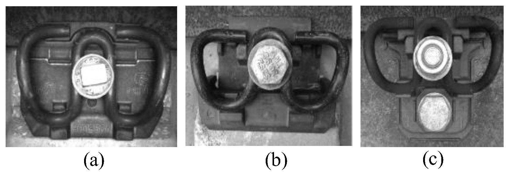
Figure 2.
Structure and clip gap of WJ-8 type of fastener.
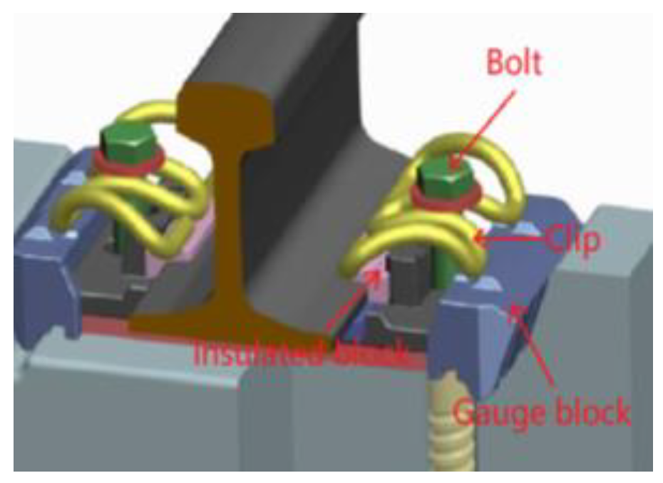
Figure 3.
Common defects of fastener. (a) Skewed clip. (b) Bolt missing; (c) Fastener missing.;(d) Over-tight fastener.
Figure 3.
Common defects of fastener. (a) Skewed clip. (b) Bolt missing; (c) Fastener missing.;(d) Over-tight fastener.

Figure 4.
Flowchart of our method3. Methodology.
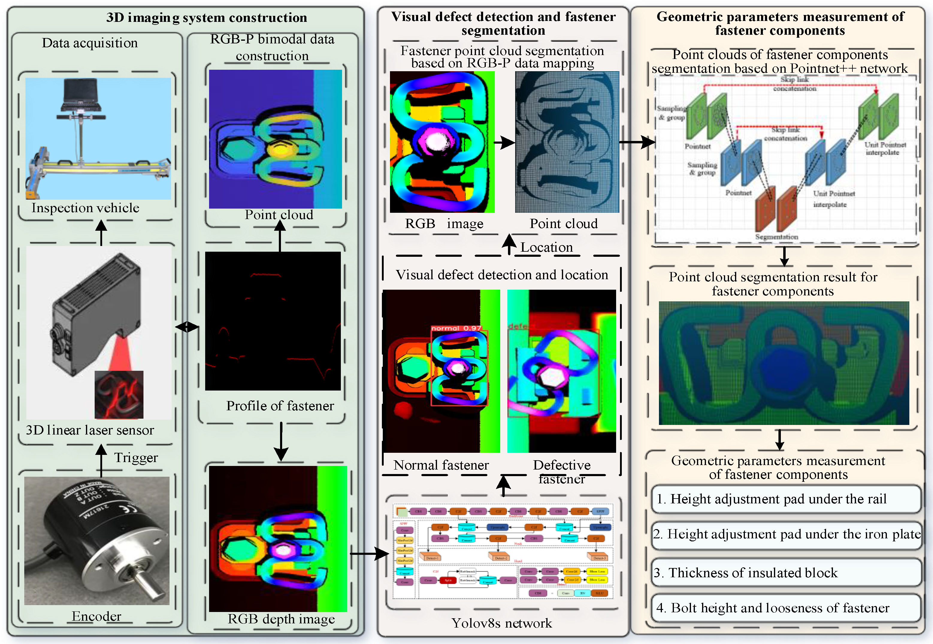
Figure 5.
Principle and physical of railway 3D imaging system based on 3D linear laser sensor. (a) The principle of railway dynamic scanning of 3D imaging system; (b) Physical of railway fastener 3D imaging system.3.1.2 RGB-P Bimodal Data Construction.
Figure 5.
Principle and physical of railway 3D imaging system based on 3D linear laser sensor. (a) The principle of railway dynamic scanning of 3D imaging system; (b) Physical of railway fastener 3D imaging system.3.1.2 RGB-P Bimodal Data Construction.
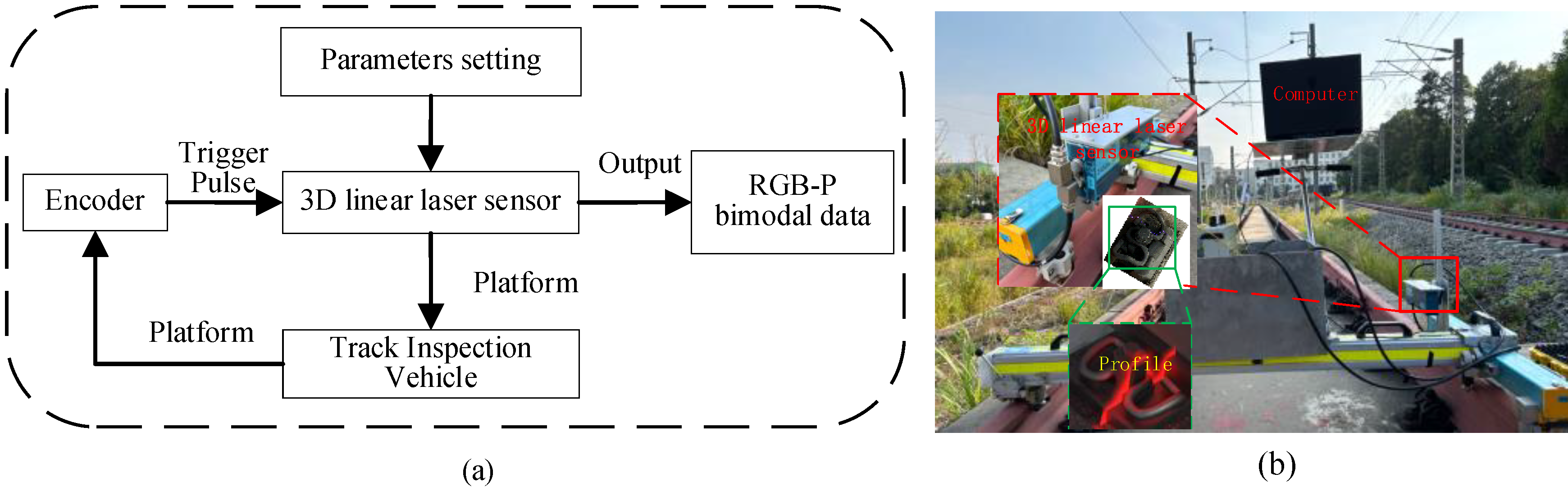
Figure 6.
RGB-P bimodal data of railway. (a) RGB depth image. (b) Point cloud rendering for display.
Figure 6.
RGB-P bimodal data of railway. (a) RGB depth image. (b) Point cloud rendering for display.
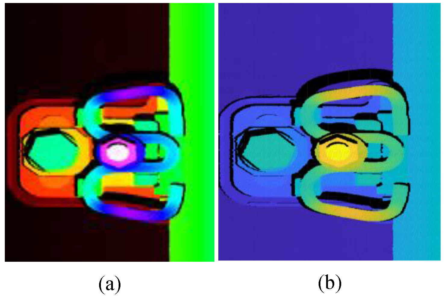
Figure 7.
Fastener detection and location results. (a) and (b) are visually normal fasteners, (c)-(d) are visual defects of fasteners.
Figure 7.
Fastener detection and location results. (a) and (b) are visually normal fasteners, (c)-(d) are visual defects of fasteners.
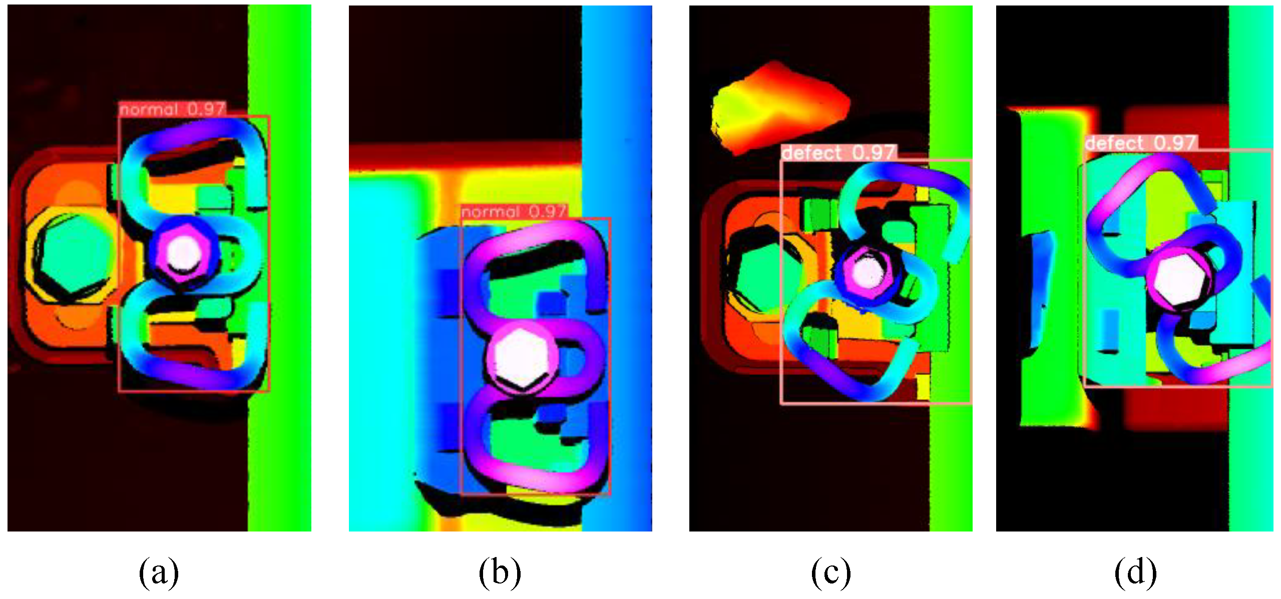
Figure 8.
The flowchart of fastener point cloud segmentation based on RGB-P bimodal data mapping3.3 Point cloud Segmentation and Geometric parameters Measurement of Fastener.
Figure 8.
The flowchart of fastener point cloud segmentation based on RGB-P bimodal data mapping3.3 Point cloud Segmentation and Geometric parameters Measurement of Fastener.
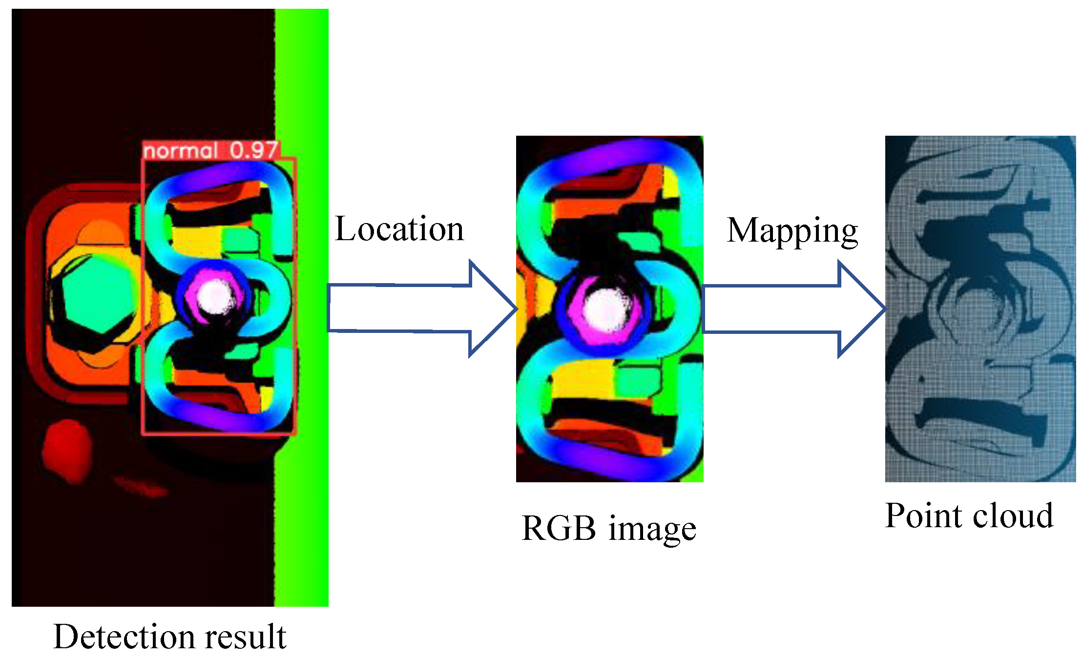
Figure 9.
PointNet++ network architectureThe point cloud dataset was manually annotated with component-wise labels to facilitate supervised training of the PointNet++ network. Figure 10 illustrates the annotated point clouds, where distinct colors denote different fastener components. The numerical annotations (① through ⑧) correspond to: bolt upper surface, metal clip, insulated block, iron plate upper surface, gauge block upper surface, rubber pad upper surface, rail edge, and sleeper upper surface, respectively.
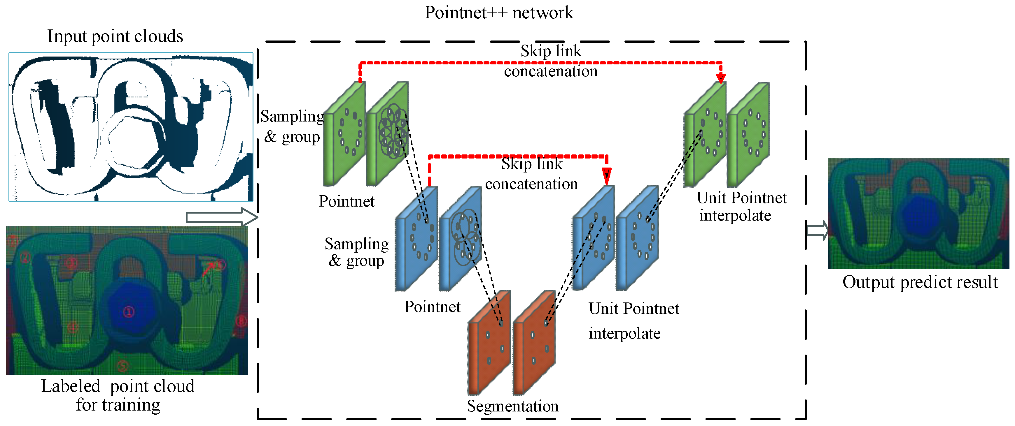
Figure 10.
Geometric parameters measurements of the WJ-8 fastener: (a) detailed structure diagram of WJ-8 fastening system. (b) in-situ image of fastener; (c) point cloud of fastener. A: insulated block; B: rubber pad; C:metal clip; D: gauge block; E: buffer pad; F: embedded brushing; G: bolt; H: flat washer; I: height adjustment pad under the rail; J:iron plate; K: height adjustment pad under the iron plate. ①: upper surface of the bolt; ②: metal clip; ③: insulated block; ④: upper surface of the iron plate; ⑤: upper surface of the gauge block; ⑥: upper surface of the rubber pad; ⑦: rail edge; ⑧: upper surface of the sleeper support.
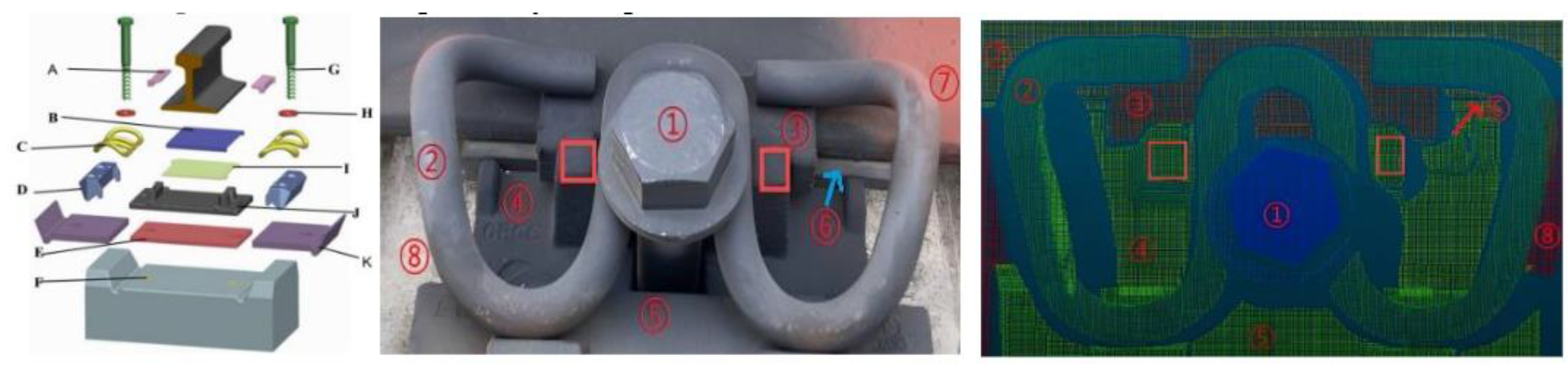
Figure 11.
The installation and structure of the gauge blocks.
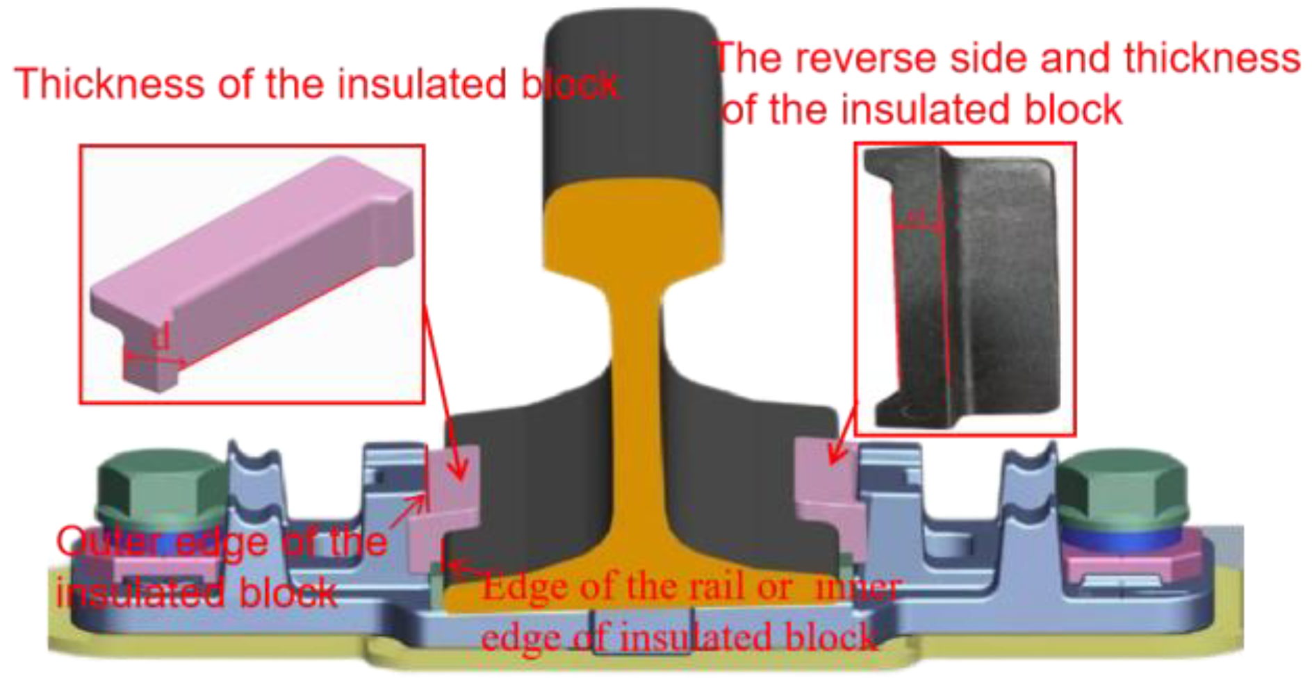
Figure 12.
The 3D linear laser sensor scanning the standard block for analyzing the measurement accuracy of the 3D imaging system. (a) is schematic of standard step block; (b) is schematic of standard block imaging; (c) is point cloud of step block; (d) is measurement error of block4.2 Accuracy Analysis of Visual Defect Detection and normal fastener location.
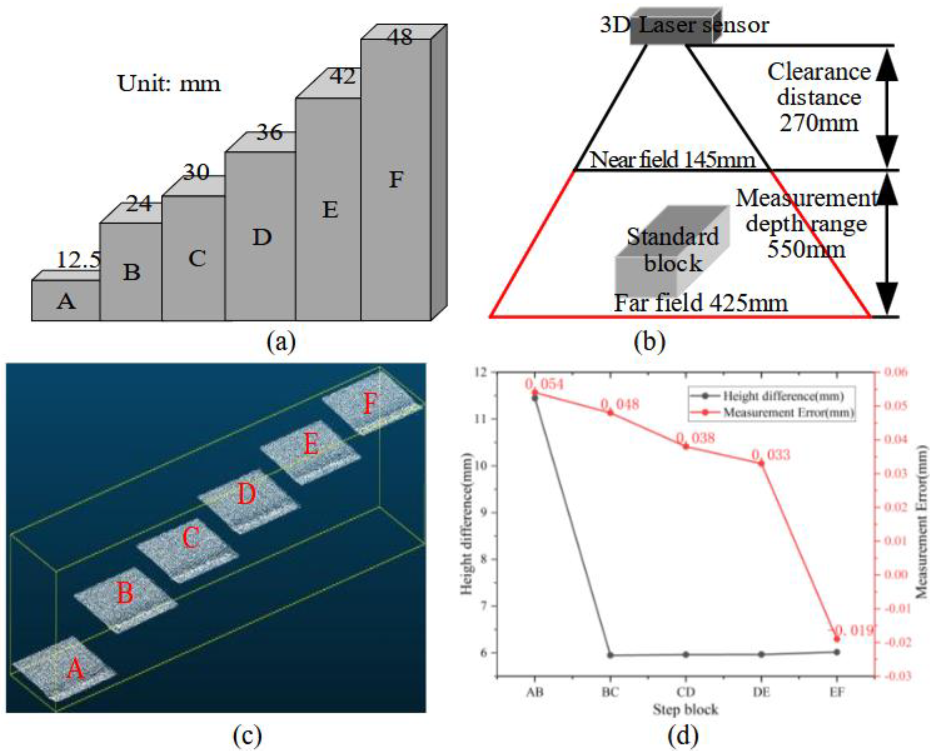
Figure 13.
Fastener detection results based on Yolov8s model. (a) and (b) are the visually normal fasteners of WJ-8 and WJ-7 type of fastener respectively; (c) is the loose fastener with the clip having the same shape as that of the normal fastener; (d) is a visually normal fastener located on ballasted tracks; (e) is the visually defective fastener with its clip slightly tilted.
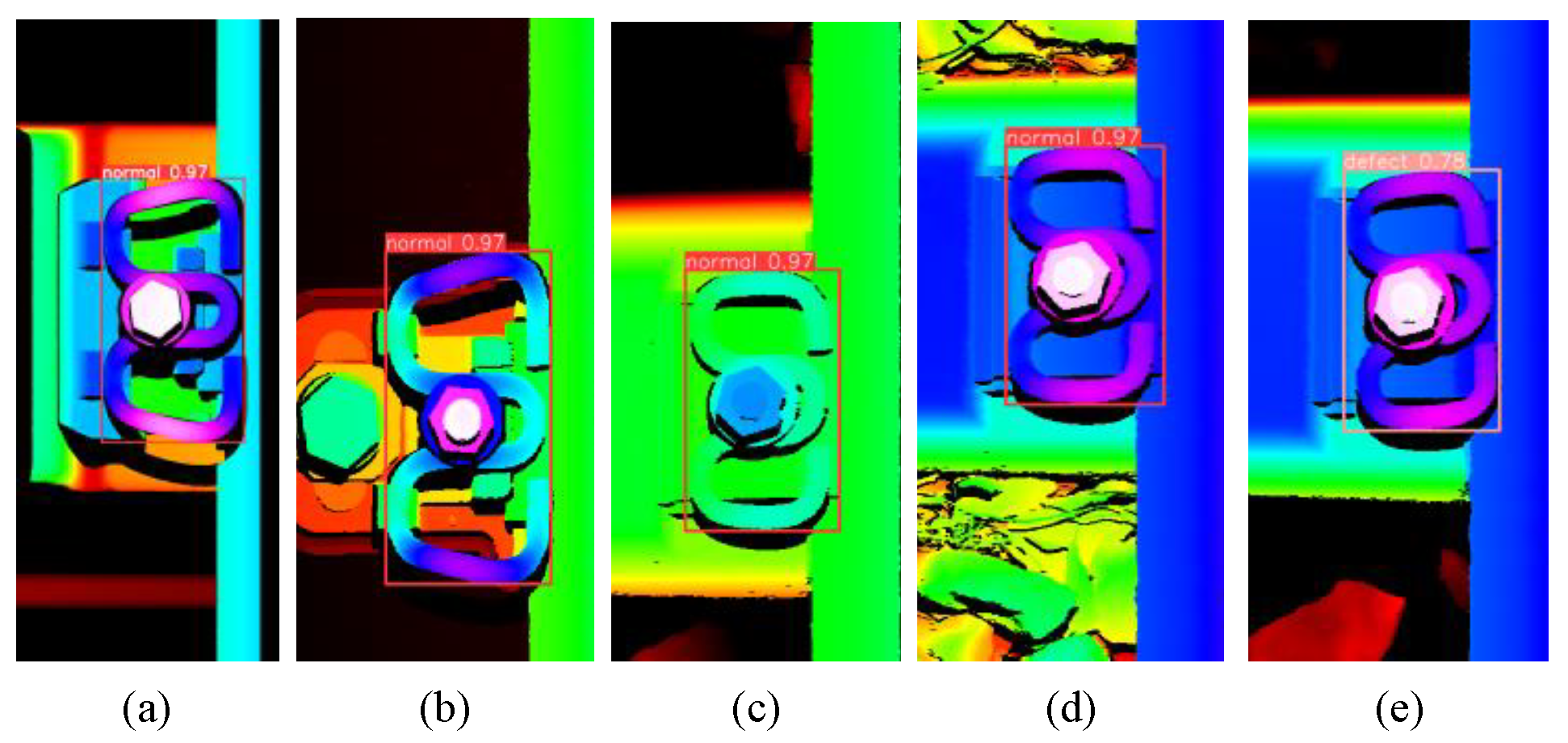
Figure 14.
The IoU of visually normal fastener location based on Yolov8s network.
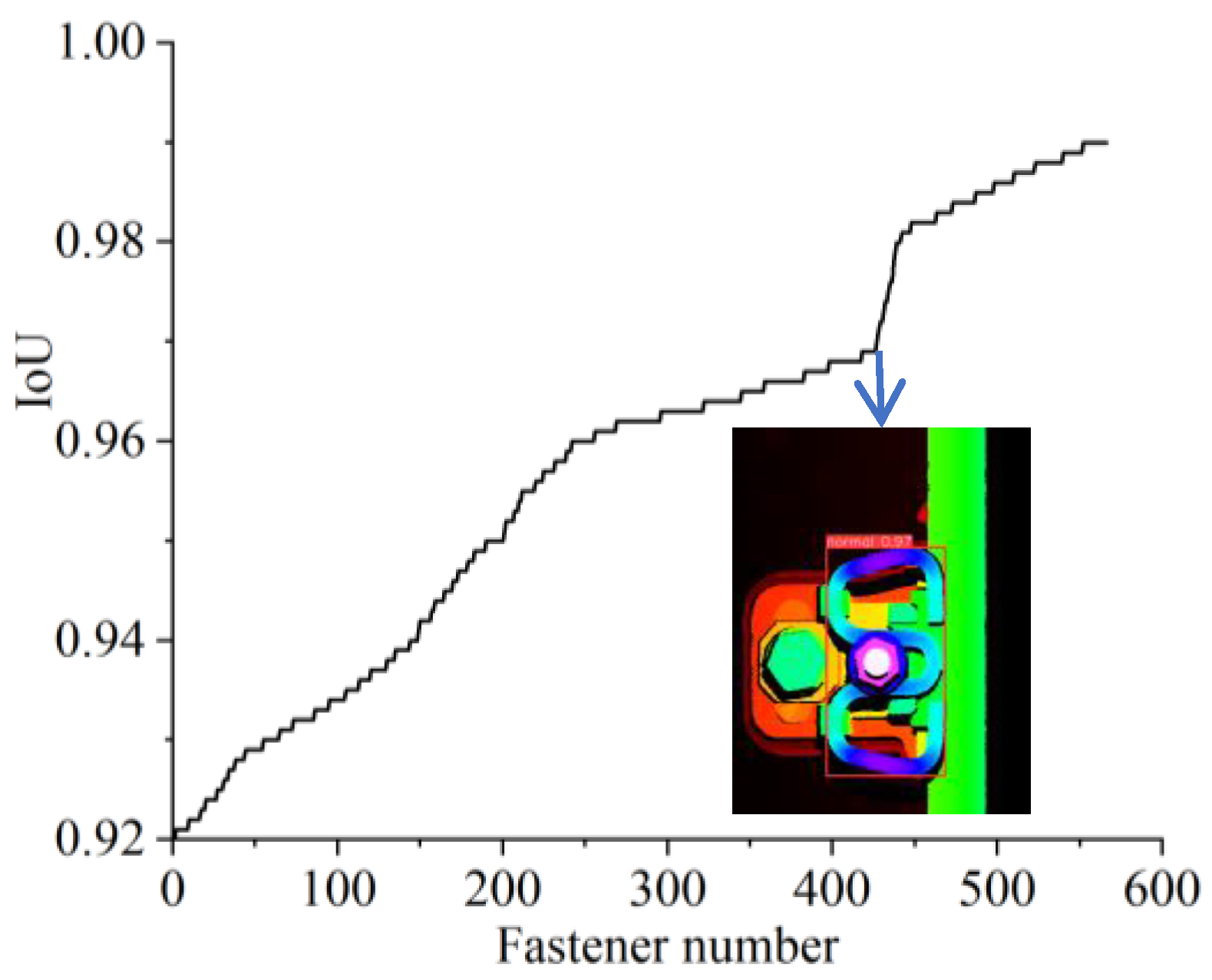
Figure 15.
The IoUs of fastener components segmented by Pointnet++ network.
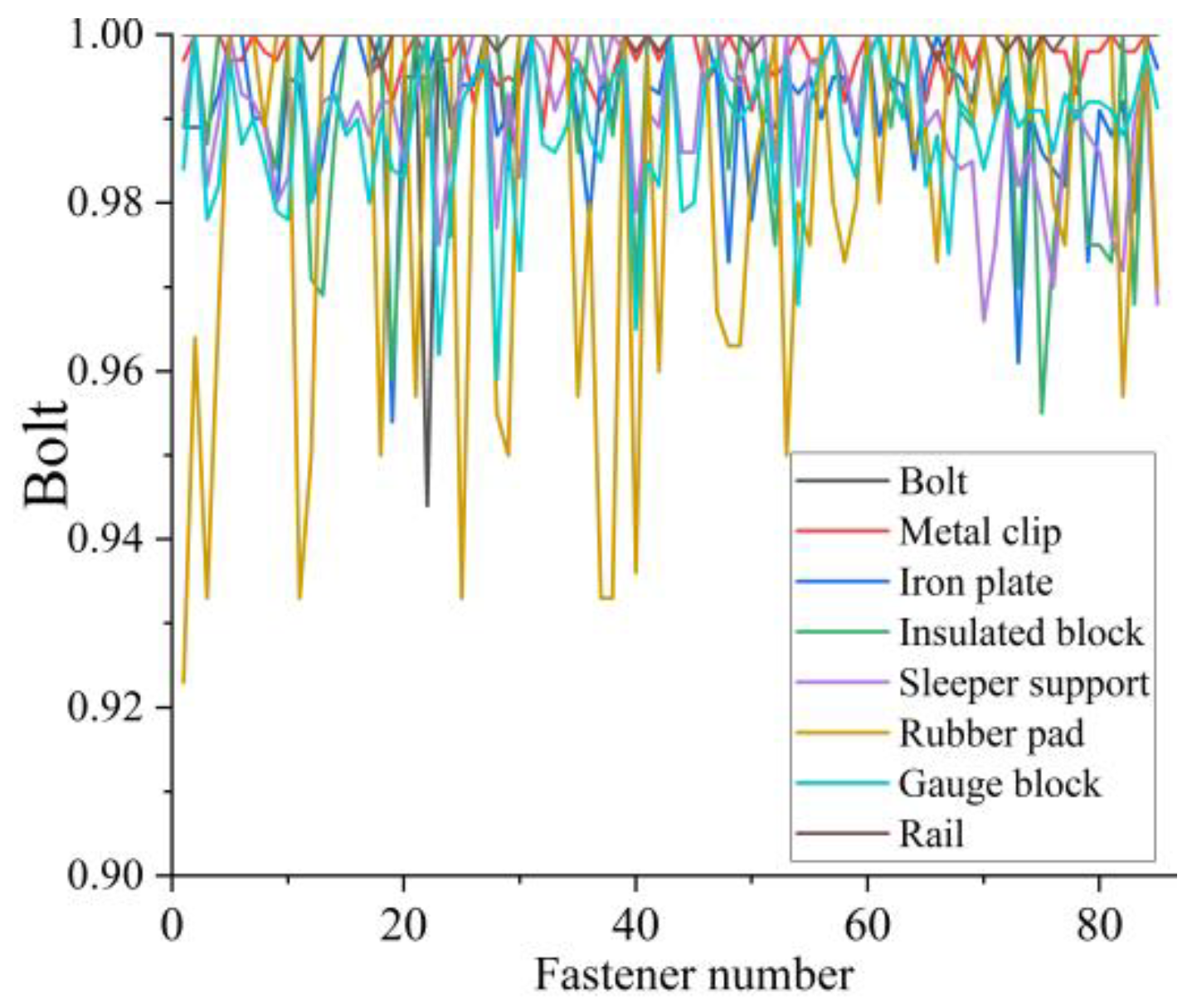
Figure 16.
The fastener point cloud segmentation results based on the Pointnet++ network.
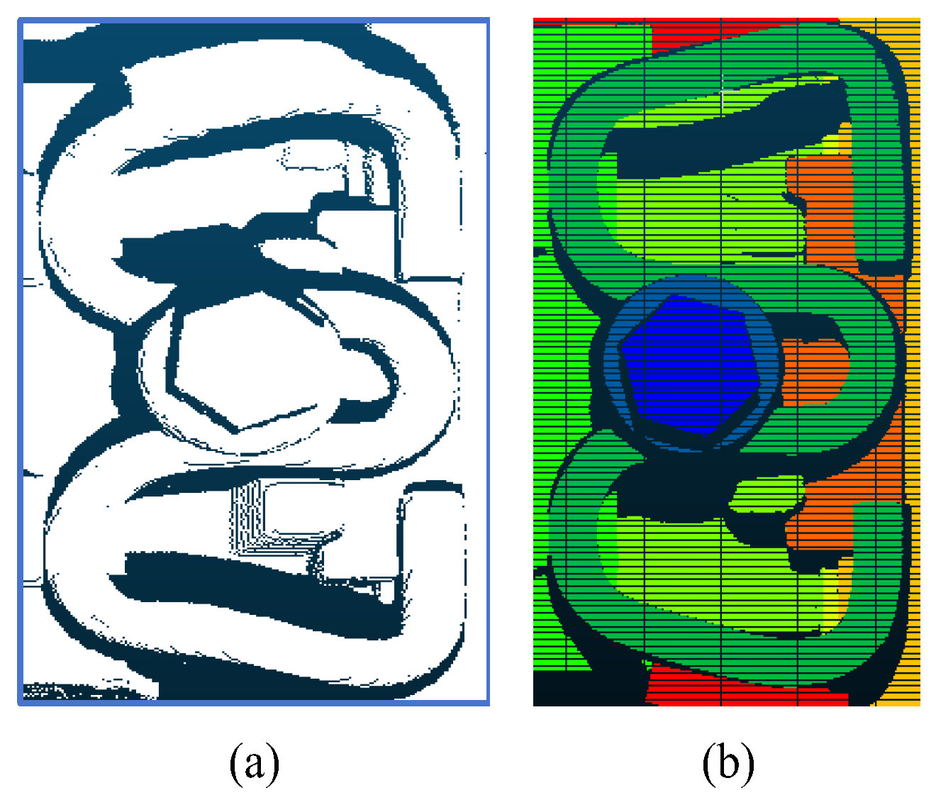
Figure 17.
The measurement results of height adjustment pad. (a) The height pad under iron plate; (b) Height pad under rail.
Figure 17.
The measurement results of height adjustment pad. (a) The height pad under iron plate; (b) Height pad under rail.
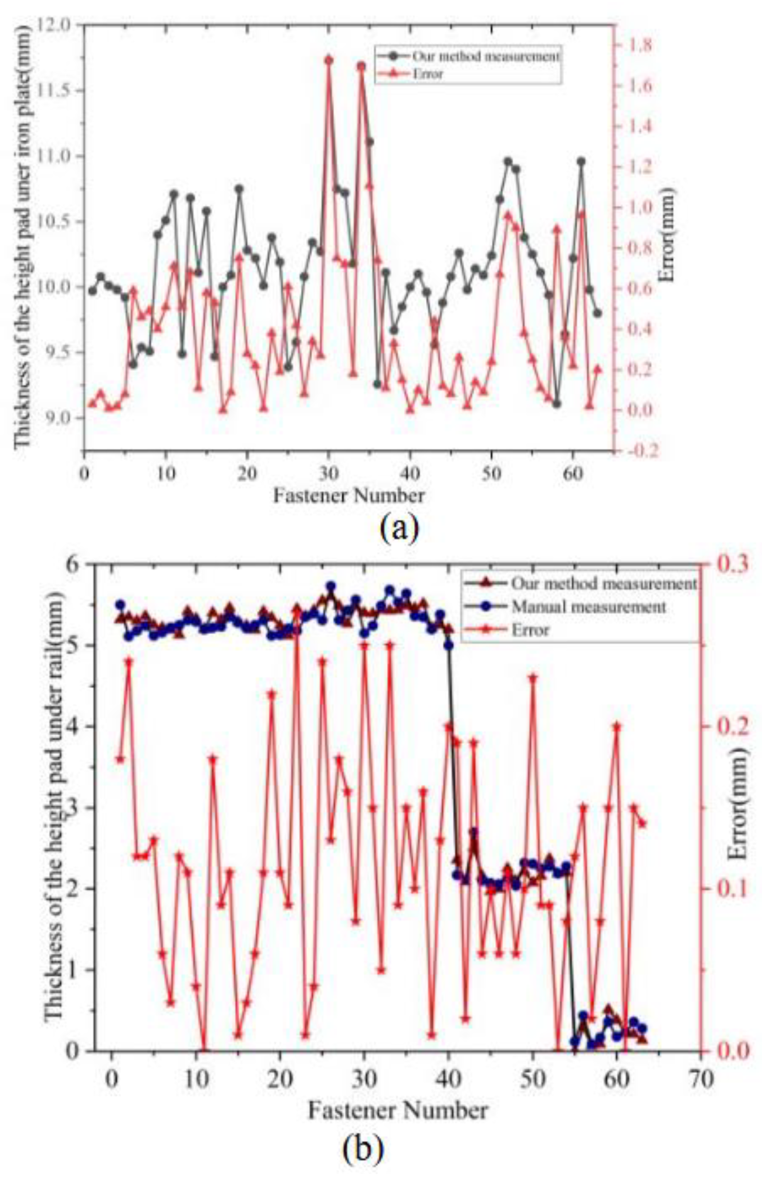
Figure 18.
The measurement error with different dx for the specification of insulated block.
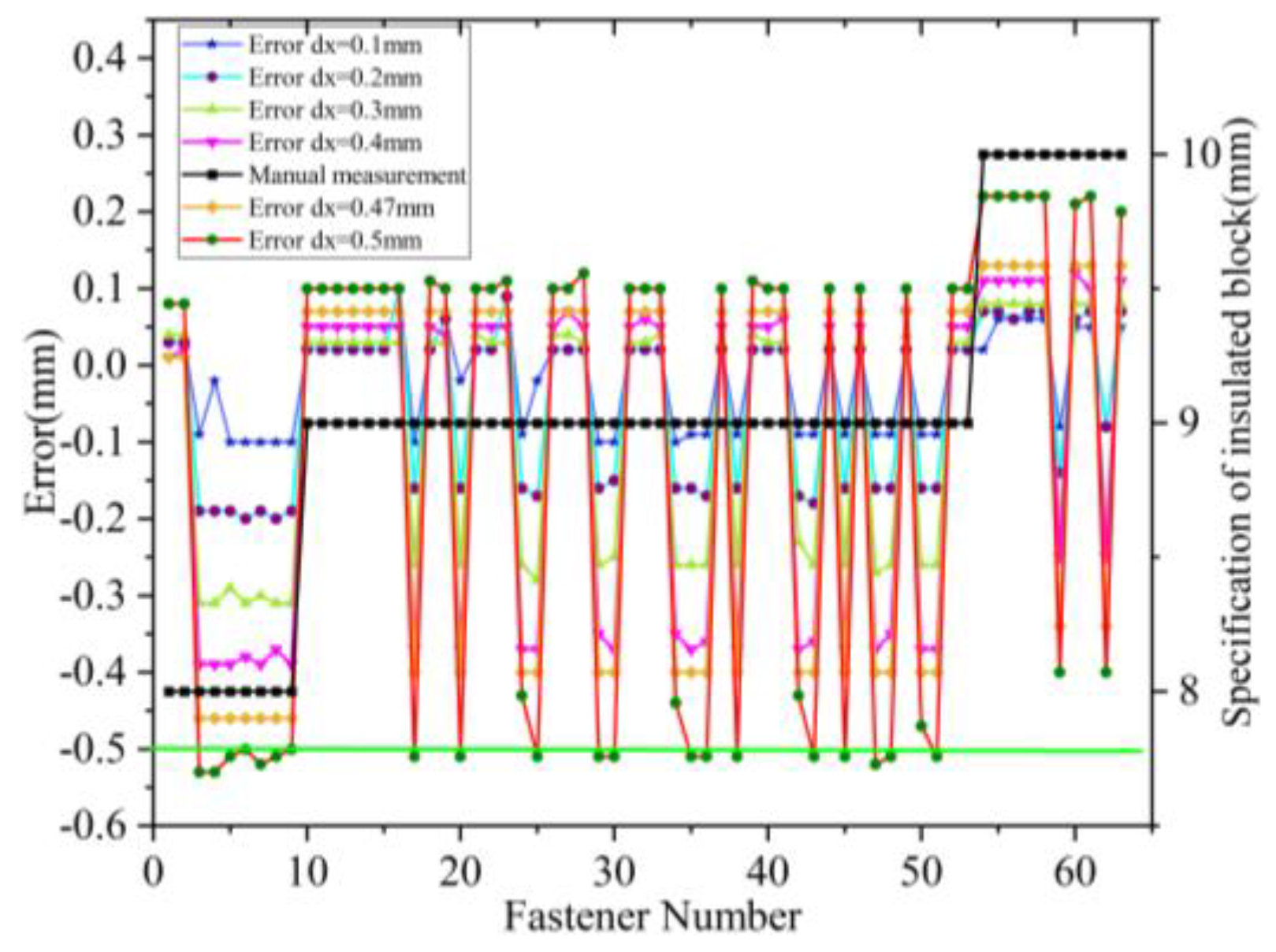
Figure 19.
The measurement bolt height for different fastener.
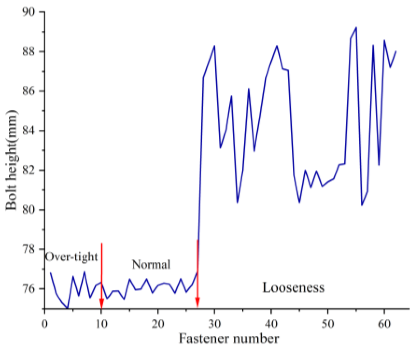

Table 1.
The hyper-parameters used for Pointnet++ network training.
| Item | parameters | value |
| Network training | Sample number | 84 |
| Batch size | 16 | |
| epoch | 251 | |
| Learning rate | 0.001 | |
| Step_size | 20 | |
| Lr_decay | 0.5 | |
| Number point(npoint) | 2048 | |
| Adam algorithm | momentum | 0.9 |
| betas | 0.999 | |
| eps | 1e-08 |
Disclaimer/Publisher’s Note: The statements, opinions and data contained in all publications are solely those of the individual author(s) and contributor(s) and not of MDPI and/or the editor(s). MDPI and/or the editor(s) disclaim responsibility for any injury to people or property resulting from any ideas, methods, instructions or products referred to in the content. |
© 2025 by the authors. Licensee MDPI, Basel, Switzerland. This article is an open access article distributed under the terms and conditions of the Creative Commons Attribution (CC BY) license (http://creativecommons.org/licenses/by/4.0/).
Copyright: This open access article is published under a Creative Commons CC BY 4.0 license, which permit the free download, distribution, and reuse, provided that the author and preprint are cited in any reuse.


