Submitted:
21 March 2025
Posted:
26 March 2025
You are already at the latest version
Abstract
Particle in Cell (PIC) simulation has been used to validate a conceptual design for a quasi-spherical, net power, hydrogen plus boron-11 fueled, fusion reactor incorporating high temperature superconducting (HTS) magnets. By burning a fully thermalized plasma, our proposed MET6 reactor uses the principles of Magneto-Electrostatic Trap design of Yushmanov (1980) to improve the classic Polywell design, resulting in a predicted power-balance Q ≈ 1.3. Because the input power consumed by the reactor will barely balance the waste bremsstrahlung radiation, future research must focus on reducing the bremsstrahlung losses to reach practical net power levels. A first step to reducing bremsstrahlung, explored in this paper, is to tune the reactor parameters to reduce the trapped electrons energies.
Keywords:
fusion reactor design
; Particle-In-Cell simulation
; power-balance
1. Introduction
This paper reports on a conceptual design process aimed to produce a net-power fusion reactor constructed with six high-temperature-superconducting (HTS) electromagnets. Computer simulation results were analyzed using Yushmanov’s magneto-electrostatic-trap (MET) theory [1]. Our spherical design, which we named MET6, has a more efficient shape for plasma confinement than cylindrical designs. Yushmanov showed that, considering only particle losses, power-balance (Q) scales linearly with the volume-to-surface ratio of a confined plasma core. Since a sphere has a bigger volume-to-surface ratio than a cylinder of the same volume, our spherical design might be expected to produce larger Q-values than recent cylindrical ones [2,3], but only if its electron-boron bremsstrahlung loss can be kept to manageable levels.
In addition to bremsstrahlung loss, a second potential source of radiation loss has also been considered and found negligible. Synchrotron radiation will be emitted from any magnetized portions of the plasma volume. But due to diamagnetic cancellation inside the plasma, magnetic field with plasma may exist only in a relatively thin sheath layer at the surface of a trapped plasma ball [1]. Not only does the sheath occupy a small portion of the reactor volume, but any synchrotron radiation emitted from it is in the infrared/microwave region of the optical spectrum, making it possible to absorb the synchrotron radiation inside the reactor, thereby preventing its loss [4]. For these reasons, namely limited volume and low photon-energy, the loss of energy via synchrotron radiation can be justifiably ignored compared to the losses due to the higher energy bremsstrahlung radiation.
Yushmanov’s analysis was specialized to reactors burning deuterium plus tritium (DT) fuel. Because of concerns for the long-term availability of the rare isotope tritium [5,6], we have chosen to design a reactor burning hydrogen plus boron-11 (pB11) fuel. Compared to tritium, terrestrial B11 is so plentiful that supplying it to future generations will not substantially increase the operational costs of the MET6 reactor. Natural boron is 80% comprised of the isotope boron-11. In our analysis, we compute reactor power-balance to serve as a figure of merit in comparing various reactor designs. Power-balance is defined as the ratio of usable-power-output to the drive-power-input. Drive-power-input is what’s needed to confine and heat the fuel plus what’s needed to compensate for heat lost to bremsstrahlung radiation. Because of the relatively high 5+ charge state of the boron-11 in the fuel, our power output is dominated by useless bremsstrahlung radiation overpowering fusion power output. For this reason, the quest for a practical pB11 reactor design shifts to the need to reduce the bremsstrahlung losses as opposed to the DT reactor’s designs’ focusing on reducing particle losses.
Reactors burning DT fuel are little troubled by bremsstrahlung radiation. It is even ignored in the analysis of Yushmanov [1]. On the contrary, in our case, we can approximate the minimum input-power requirement to be just that needed to balance the bremsstrahlung losses. This simplifies the calculation of power input which can now be computed from a textbook formula for bremsstrahlung power. The resulting power-balance is predicted to be 1.3, just barely into break-even range.
The design still holds promise as a contender for commercial power because the predicted power-balance depends on the reactor’s many design parameters, most of which have not been systematically explored. For example, the best footprint for the HTS magnets is unknown, pending future development by HTS magnet designers, e.g. Commonwealth Fusion Systems of Massachusetts. In lieu of a specification for a workable HTS magnet, we chose to adopt the footprint of a commercially available resistive magnet [7]. The simulated footprint of the magnet affects the design’s performance in a complex way. The surfaces of the four magnets mounted on the four side-faces of the cube intersect the simulation plane in the eight square boxes shown in each panel of Figure 1(a-c). The bias voltage applied to the magnets creates a complicated equipotential surface determining the E-field throughout the simulated plane. The shape of a resistive magnet is normally optimized to facilitate water-cooling through hollow-wires wound on a cylindrical central spool. HTS magnets would be optimized differently, producing a different E-field from the resistive design. The design of our HTS magnets would include features chosen to maximize the power-balance via computer simulation.
MET6 evolved naturally from its predecessor, the hexahedral Polywell reactor, invented by Robert Bussard in 1989 [8]. Bussard’s Polywell design was effectively criticized by Rider in 1997 [9] and again in the 2018 Jason Report [10], summarizing the U.S. Department of Energy’s ARPAE funding program. The Jason Report concluded that Polywell was “unlikely to reach scientific break-even” referencing Rider [9] and Rostoker et al. [11]. Rostoker et al. had shown convincingly that Rider had wrongly assumed impossible operating conditions, making his conclusions inapplicable for practical reactor design.
The design of our MET6 sidesteps this controversy [9,11] over Polywell’s claim to a non-thermal energy distribution. In contrast to Polywell, the plasma in our MET6 reactor is predicted to have a Maxwellian (i.e. thermal) energy distribution, with only a slight departure predicted due to the extreme high energy tail of electrons up-scattering to energies exceeding the height of the trapping potential. This minor departure from Maxwellian distribution was ignored by Yushmanov [1], Dolan [2] and Sporer [3] and likewise in this paper. Pure Maxwellian energy distribution is a specified feature of the MET6 design.
2. Hardware Design
MET6 is a fusion reactor designed around six cylindrical, HTS coil-magnets mounted on the faces of a regular hexahedron (i.e. cube). Figure 1(a-c) shows PIC [12] simulated snapshots of the plasma in the central plane of the cube. Individual macro-particles’ positions are plotted as black dots, electrons in (a), protons in (b), and boron-11 ions in (c). When the simulation program runs, it displays a new snapshot of the particle positions at each time step, i.e. every 73 picoseconds of plasma time. Analysis of the particle movements guided our optimization of the design. The most important parameter of the design is the size of the magnets, which determines the resulting size of the cubic vacuum tank and the diameter of the plasma ball enclosed by the magnets. The fusion power scales with this size in proportion to the volume of the vacuum tank, labeled ① in Figure 1(a). The tank is required to be big enough to leave clearance outside the ring of magnets to accommodate insulating, hollow legs supporting the magnets from the tank. The legs are not shown, but the simulation predicts clear spaces left to accommodate the legs without causing plasma losses. The invention of hollow, insulating support legs and clear-space to accommodate them is the subject of a 2015 patent on a proposed Polywell reactor [13]. Although our MET6 reactor does not function like Polywell was supposed to [8], the support legs would be the same as described in the patent. The magnets in Figure 1 appear to be floating in space but 8 areas clear of plasma are predicted by the simulation to occur between the magnets and the nearest tank wall. These clear spaces were designed to accommodate non-intercepting support legs which would reach from the tank wall to each of the eight magnet boxes shown.
Figure 1(a-c) shows the major internal components of the reactor labeled with circled integers as follows: ① labels the square cross section of the cubic vacuum tank, of diameter 4.79m and shown with tick marks. The metal tank is simulated as an electrical conductor held at zero volts. The tank serves as a grounded cathode for injecting electrons, protons, and boron fuel ions. ② labels the location of an electron emitter, envisioned as a hot filament biased to the same zero voltage as the tank. Starting at time t=0, 15 amps (A) of zero-energy electrons were simulated from the point source depicted as an orange dot located 1 cell width (= 9.57cm) inside the right-hand tank wall in panels (a-c). Electrons are accelerated inward by an electric field formed by applying a 2.4 megavolt (MV) DC voltage to 8 conducting magnet boxes serving as an electrical anode. The square boxes labeled ③ and ④ represent one of the four magnet coils mounted on the four side-faces of the cube. Three other pairs of boxes represent the other three magnets surrounding the central plane of the cube. Each coil intersects the central plane in two areas, outlined by square boxes. At the approximate center of each box is simulated a long straight HTS wire carrying current appropriate to generate the magnetic field required to confine electrons as shown in Figure 1(a). The location of each of the 8 wires was adjusted to be no less than ½ cell-width from the geometrical center of its nearest magnet box. Such adjustment was necessary to avoid calculating the field too near a singularity in the field-expression when evaluated at zero distance from a wire.
Choosing to locate the 8 wires near but not too near the centers of the boxes is a simplification made to facilitate the tabulation of B-field values for each cell. The x- and y-coordinates of static B-field were computed separately and stored as two 50x50 arrays in memory. A real-world superconducting coil would have wires filling the area inside each box. The power-balance from a reactor with such real coils will differ by an unknown amount from the one calculated from our simulated coils. This difference is the main uncertainty in the simulation.
Starting at time t=0, electrons flow continuously into the center of the tank through the open bore of the right-hand magnet coil i.e. between squares labeled ③ and ④. The trapped electrons’ density increased with time until it reached the spatially uniform density shown in snapshot (a), made at a plasma time of t=0.38ms. This time was chosen as a stopping point for the simulation. It is the earliest time that the plasma density reached a stable, steady-state condition. As long as the electron drive current was held at 15A the plasma density was constant, independent of time.
This density is still many orders-of-magnitude too low to produce net power. In real-world start up, the electron drive current and matching ion injection currents would be increased over time to raise plasma density to net-power levels. In the simulation, the diagnostics at this early time are enough to predict the net-power conditions, making it unnecessary to explicitly simulate beyond t=0.38ms. A key finding is that the shape of the plasma core is constant in simulated time so that the net-power density could be determined by the β=1 condition that defines the same surface at net-power as we see in Figure 1. From the Plasma Formulary [14], the formula for β = (4e-11)nT/B is a function of electron density n, temperature T, and magnetic field B, all evaluated at the surface of the plasma core. The β=1 equation was inverted to find the surface electron density n, which also must equal the surface fuel density due to the requirement for quasi-neutrality. Figure 1(b-c) show the fuel density to be uniform inside the surface. The fuel density determines the reactor’s power output and, dividing it by the drive power, the power-balance, which is the key measure of reactor performance.
In a real reactor, the magnetic field internal to the plasma sheath would become zero as the density rises toward β=1. In the simulation, at the time of Figure 1, the plasma density was still too low to generate any significant diamagnetic field. To help speed the calculation, the OOPIC simulation was run using the “electrostatic” mode, in which the magnetic field is static in time and initialized cell by cell from programmed expressions. To simulate diamagnetism, the t=0 field from the HTS wires was replaced cell-by-cell with a zero value for all cells inside a square region of cells spanning the center of the tank. Outside the region the field was computed from the textbook formula for fields from 8 infinitely-long wires. The width of the field free region is indicated by the double-headed arrow in Figure 1(a). The diameter of the region was used as an adjustable parameter, adjusted to match the width of the recirculating electron beam to just fill an aperture at the position of the vertical arrow in Figure 1(a). The wider was the field free region selected, the wider was the beam width at the aperture. The wider the beam at the aperture, the greater the current of electrons scraped off by the aperture.
Ions enter the tank from two point-sources, protons from a source located at position ⑤ in Figure 1(b) and boron ions from a source at position ⑥ in Figure 1(c). Positions of the point-sources were fixed at the center of the left-hand tank-wall and the velocities/currents of the ions specified by adjustable parameters in the input file. The velocities were adjusted by trial and error for the ions to pass freely into the core of the reactor along the cusp line through the bore of the left-hand magnet. The currents were adjusted to stabilize the densities of the two species of ions to form charge densities equal to each other and each matching half the electrons’ charge density.
The design of ion sources for tokamaks is the subject of others of our papers [15,16]. Injection into tokamaks is more demanding than into MET6 due to the tokamak’s transverse magnetic field, which tends to deflect charged-particle beams. To avoid such deflection, tokamaks require neutral or neutralized beams whereas MET6’s cusp injection works well with simpler charged particle beams, i.e. those simulated here. As seen in Figure 1(b-c) the ions incoming from the sources ⑤ and ⑥ are focused into narrow beams by the cusp field in the left-hand magnet.
On entering the tank, newborn ions travel through the open bore of the left-hand magnet. The initial energies of the ions, selectively imparted by the sources, were chosen to just exceed the peak of decelerating potential they will find on entry. Figure 2(d) shows a graph of the steady-state potential function along the horizontal midline of the reactor, the path followed by ions on their first pass through center. The shape of this potential function is crucial to the functioning of the reactor. It determines the temperatures of the electrons’ and ions’ plasma. Yushmanov [1] presented a similar potential function for his hypothetical toroidal multipole with 10 anode gaps. Yushmanov identified its main characteristics as a central potential minimum at half the bias voltage U and trapping of electrons in the potential wells represented by the inversion of the two peaks. The trapped electrons depress the maximum potential voltage by an amount Yushmanov called ΔU. The remaining potential he divided equally to produce equal electron and ion temperatures. In our design, the temperatures of electrons and ions may be unequal and manipulated to reduce the level of bremsstrahlung losses.
The force on a newborn ion is proportional to the negative gradient of the potential shown. The ions’ initial velocities are slowed by the rising slope of the potential until they reach the left-hand peak of the potential, where the force is zero. The ions residual momentum carries them into the core, down the falling slope of the potential well. They accelerate to the tank-center, where the force is again zero. To the right of center, they decelerate until they reach the right-hand peak, marked “U-ΔU = 2.2MV” in Figure 2(d). At this point, they reverse direction and turn back to the left. To avoid loss of newborn ions to the right-hand tank wall, their initial kinetic energies were chosen to be slightly less than the potential energy e(U- ΔU), which subtracts from their kinetic energy at the top of the right-hand peak.
To visualize the ions’ early history, their positions in velocity-position phase space are displayed in Figure 2(e); here, gray dots represent protons and black dots represent boron ions. The upper arrow marks the incoming paths of protons and the middle arrow marks the incoming path of the boron ions. Due to their different charge-to-mass ratio, boron ions follow a different path than protons of the same energy. Due to their higher charge state, boron ions scatter more and become trapped more often than the protons on their first pass. Most protons are seen to reflect from the rising potential they experience in the right-hand magnet and then exit the tank to the left after a single pass forward and back through center. The bottom arrow shows the exit path of protons; it is more densely populated than the boron ions’ exit path just above it because more protons survive trapping on their first pass than boron ions.
The stopping conditions of the simulation leading to the diagnostics at this time t=0.38ms were determined by the condition that the particles’ densities stabilized in time and the ions’ positive charge density approximately cancel the electrons’ negative charge density at the center of the reactor. The ion injection currents were adjusted to make the sum of the 2 ions’ central density values, Figure 1(e) plus (f), approximately equal to the electrons’ central density value, Figure 1(d). This condition made the central plasma approximately charge-neutral, with only a slight excess of negative charge. The visible discrepancy between the level of the proton charge density in (e) and boron charge density in (f) is accidental, due to random statistical variations in cell counts. The curves in (e) and (f) are subject to relatively large statistical noise because they represent charges in a horizontal row of cells only one cell wide in the vertical direction. For this reason, each cell contains only a few macroparticles, and consequentially the exact number is subject to relatively large statistical uncertainty. The apparent discrepancy between proton and boron densities does not affect the predicted power-balance of the reactor which is determined by the ratio of bremsstrahlung power to fusion power at the final electron temperature. Making the proton and boron charge densities equal was adopted for simplicity, later found to be non-optimum for power-balance, as described in the discussion of equations (1) and (2) in the next section of this paper.
The electrons formed the 2D electrostatic potential color coded in Figure 2(a). The (online published) colors code the potential voltage; magenta codes the applied voltage of 2.4MV, found uniformly inside the 8 magnet boxes. Light-blue codes the tank-central value of potential, 1.2MV, half the applied voltage. Red codes voltages near zero, outside the ring of magnet boxes and extending to the tank walls. Figure 2(d) shows a 1D graph of the potential voltage made along the horizontal midline of the 2D plot (a). The central value is half the applied voltage, a feature found in the original MET reactor concept [1]. In our simulation, the depth of the potential well was found to vary with the selected electron injection current. We initially adjusted the electron injection current to be 15A, to produce a potential-well depth equal to half the drive voltage and to agree with Yushmanov’s analysis [1]. This 15A drive current produced equal ion and electron temperatures, a restriction adopted by Yushmanov as a simplifying assumption. The restriction to equal temperatures was relaxed in our later analysis. We reduced electrons’ temperature below ion temperature as a means to reduce bremsstrahlung and thereby increase power-balance. Although the individual electrons in Figure 1(a) are in constant motion, the potential they form is static in time from t=0.38ms on. The stopping condition of the simulation was chosen to make the ions’ positive charge-density to be slightly less than the negative charge-density of the electrons. This made the central potential nearly the same with or without ions injected. At steady state, the electrons’ charge density was partially neutralized by the trapped ions, but a slight negative charge was intentionally left to keep the attractive potential approximately the same as it was before injected ions began to accumulate.
The magnetic field from our six-magnet reactor is dominated by cusps. Figure 2(b) shows a rendering of the magnetic field’s equal-magnitude surface in a six-magnet Polywell constructed at the University of Sydney [17]. The size of our simulated reactor is bigger than the Sydney one, but the shape of the magnetic field is the same. The shape is dominated by 26 cusp lines, a selected three of which are marked by arrows in (b). Charged plasma particles travel freely along the cusp lines, undeflected by the parallel magnetic field vector. This feature allows controlled injection of charged particles from electron, proton, and boron sources mounted at either ends of the horizontal cusp line.
Unfortunately, the 26 cusp lines also provide 26 paths for hot plasma particles to escape the core and (some of which) become lost by hitting the tank walls. The simulation software is, by design, two-dimensional which requires selecting a plane through the cube in which to simulate the features also relevant to a 3D plasma. The plane selected is the cube’s central plane, outlined by a square of solid and dashed lines in Figure 2(b). This plane contains face and edge cusps, typical ones of which are indicated by the two lower arrows in (b), but none of the cube-corner-vertices, a typical one of which is indicated by the upper, left-pointing arrow. The cube’s 8 corner-vertices are out of the central plane and therefore their losses are not simulated. By this omission, the simulation ignores the losses through the cube-corner-vertices but includes the losses through the more lossy face and edge cusps. Luckily, the rate of loss of these omitted cusps, proportional to the area of the circle at the head of the left-pointing arrow, are smaller than those of the in-plane cusps, proportional to the areas of the cusps pointed to by the lower two arrows. By including the more lossy face and edge cusps in the simulation, while omitting the less lossy cube-corner-vertex cusps, we expect to overestimate the total cusp losses compared to what they would be in a more realistic, e.g. 3D, simulation. Because the bremsstrahlung losses are believed to overpower the cusp losses, the differences between loss rates through face, edge, and corner cusps do not add to the uncertainty of our estimated power-balance.
Our simplified magnetic field is simulated as if generated by electric currents in eight straight wires oriented perpendicular to the simulated plane and located near the centers of the 8 magnet boxes. The magnet boxes are simulated as metal conductors biased to 2.4MV. The biased, conducting surfaces of the 8 boxes provide the electric field which combines with the magnetic field from the wires to confine particles.
The polarity of the currents in the wires is arranged to generate magnetic field vectors pointing inward at the center-bores of each of the 4 side-facing coil magnets. The magnitude of the bore-field was adjusted to be 25 Teslas (T) at the center of an isolated magnet. The 25T field capability is the only HTS feature adopted from the specifications of commercially available HTS magnet coils [18]. When four magnets are assembled into a square, opposing fields from adjacent coils partially cancel to reduce the bore field in each magnet to 18T. The spacing of the magnets was varied by trial and error to produce the same field magnitude in the corners between the coils as in the bores. This made the recirculating electron current the same through the face and corner cusps. Static magnetic field at each PIC cell location inside the tank was computed from the textbook formula [19] for the in-plane component fields from 8 infinitely-long straight wires. Horizontal and vertical field components were computed and stored in two 50x50 arrays, one for x-field and one for y-field. The eight biased, conducting magnet boxes shown, plus eight HTS wires simulated (but not shown), combine to simulate the electric and magnetic fields from the four superconducting coils mounted on the side faces of the hexahedral reactor.
Figure 2(c) shows the x-component of the magnetic field from the 8 wires, plotted along the horizontal midline of the tank. As expected, the magnitude of the field is maximum (18T) in the bores of the two magnets on the midline and zero at the center of the tank. The field shown is the applied field which would exist prior to the injection of plasma. At steady state, the plasma modifies the central field by adding a diamagnetic current which suppresses the applied field in the central region, expanding the B=0 volume that contains the fusion fuel.
As a check that the top and bottom coils could realistically be omitted from the 2D simulation, a separate simulation of applied magnetic field was made with the public domain 3D simulation packages WarpX [20] and Magpylib [21]. The 3D simulation included six circular coil magnets on the six faces of the cube, including top and bottom coils the same size and field-strength as those in the MET6 design. In the simulation plane, the magnetic field from the 3D simulation was found to be qualitatively the same as the field from the eight straight wires, approximately matching the midline field shown in Figure 2(c). This gives us confidence that our simulated magnetic field from the eight wires captures the essential details of the magnetic field that would be found in a real cubic reactor. Although the WarpX simulation contained a realistic magnetic field, the results have not yet progressed to a level that could be used for further quantitative analysis. Our WarpX simulation so far lacks the essential biased anode, which forms an electric field that recirculates most of the escaping electrons back into the core whenever they happen to exit the central region through a cusp. Without this bias potential, the plasma would have excessive losses.
Figure 1(d) shows a graph of the electron’s particle density plotted along the midline of the 2D distribution in (a). The units of the vertical axis are electrons per square meter. Two peaks of concentrated density appear, centered in the bores of the left-hand and right-hand magnets. The right-hand peak is marked by an arrow. The peaks are concentrations of deviant electrons which have down-scattered in energy to become trapped in local minima of the electric potential formed by the bias voltage. The concentration of these trapped electrons is detrimental to the efficient operation of the reactor. By their negative charge concentration, they repel and rob energy from the newborn electrons entering from the source at position ②. To reduce the trapped electrons’ concentration, a special electrode was simulated in the bore of the right-hand magnet, as shown at the head of the arrow in (a). This electrode was simulated to describe a thin metal disk with a circular hole drilled in its center. The electrode was invented to extract a portion of the trapped electrons. The current of electrons hitting the electrode is adjusted to halt the growth of the peaks before the latest time simulated.
The current of electrons hitting the extra electrode was adjusted by varying the width of the B=0 imposed field-free region. The electron beams through the cusps are found to be broadened after crossing the field-free region. The larger the width of the region, the larger the beam widths and the larger the extracted current. Increasing the current of electrons hitting the aperture was found to reduce the height of the peaks in (d). The larger the current selected, the smaller was the concentration of trapped electrons populating the peaks in Figure 1(d). The extra electrode provides an adjustable mechanism for “pumping-out” trapped electrons, identified as necessary by Yushmanov in the following quote from his 1981 paper [22]:
“To keep the gaps 'empty' it is necessary to create in them an artificial pumping-out mechanism which has a number of specific characteristics including selectivity with respect to the trapped electrons and a carefully adjusted intensity within fixed narrow limits. No specific technical ideas for methods of creating such a pumping-out mechanism have as yet been put forward.”
Our placement of the aperture in the right-hand magnet satisfies the need to actively pump low-energy electrons, perhaps the first proposed solution since it was recognized as a need in 1981. The steady and uniform density of trapped electrons and ions in Figure 1 shows that this solution works well enough. Little effort was made to optimize the adjusted electron current loss on the aperture. Adjusting the current and power lost by the electrons hitting the electrode would impact the predicted power-balance Q, but only slightly compared to the power consumed by compensating for the bremsstrahlung losses. Such optimization of the pumping current is a detail of the design we chose to leave for future fine tuning of the design parameters. Such fine tuning was not possible using our simulation as discussed further in the “Discussion of Results” section of this paper.
In addition to providing for the pumping out of slow electrons, the extra electrode has a second important function. It shapes the potential along the path of the newborn ions to increase their probability of being trapped on their first passage through the core. The potential function shown in Figure 2(d) exhibits two peaks. The difference of heights of the peaks defines a range of injection energies suitable to choose for the incoming ions. Their injected energies need to be in a range higher than the eU value at the left-hand peak and lower than the eU value at the right-hand peak. Ions in this energy range pass freely in through the left-hand cusp and then are reflected by the potential at the right-hand cusp. This gives each ion the maximum probability of being trapped in passing twice through the bulk of the trapped plasma. Those ions not trapped on their round-trip passage exit the core to the left to be lost on the left-hand tank wall. The bottom-most of the three arrows in Figure 2(e) marks the exit path of the (gray colored) protons just above the arrow. The density of protons along the bottom-most arrow in Figure 2(e) differs from the density of boron ions on the path just above it. This is due to the different probabilities of capture of ions on their first pass forward and back through center. Because most of the newborn ions exit after a single pass, the efficiency of trapping ions from the sources mounted on the left-hand wall will improve as the central plasma density grows with time. At this early time (t=0.38ms), the injected currents of protons and boron ions were adjusted to be 2.5A and 2.75A, respectively. These currents were set by trial and error to just equilibrate the densities of newborn ions in Figure 1(e) and (f).
The distribution of the ions in Figure 2(e) reflects the history of fueling the reactor over the first 0.38ms after time zero. As simulated time increases beyond this early time, the fueling process fills in the central region of Figure 2(e), and the thermalization process degrades the ions’ initial velocities to smaller values than those shown in 2(e). After many milliseconds, the dots would accumulate densely near the center of the phase space (velocity vs. position) distribution, providing a direct measure of the final temperature of the plasma after it reaches thermal equilibrium. Rather than undertaking such an impractically long OOPIC simulation run to estimate this temperature, we relied on the analysis of Yushmanov [1], which found that thermalization lowered the plasma temperature from the applied eU to an equilibrium temperature equal to “about 1/16 of e(U- ΔU),” where ΔU is the potential depression in the gaps due to electrons’ space-charge accumulating in the gaps. From the horizontal arrow in our Figure 2(d) and the results of Yushmanov, the temperature of the thermalized plasma can be estimated as T = e(2.2MV)/16 = 140keV. The effect of thermalization is to lower the plasma temperature by a factor of 16. This estimate of thermalization loss is the main contribution of Yushmanov’s theory, which distinguishes our MET6 reactor design from the earlier Polywell designs. In Polywell theory, ions were mistakenly assumed to maintain their original eU temperature until they fused. In MET they are theoretically found to be 16 times colder.
3. Estimating the Power-balance Q from the PIC Diagnostics
The standard definition of power-balance is the ratio of fusion power output to drive power input. The fusion power output is calculated from the textbook [23] formula:
where np is the protons’ particle density, nB is the B11-ions’ particle density, <σv> is the fusion reactivity averaged over the thermal velocities (v) of the T =140keV thermal plasma, EpB = 8.7Mev, the energy yield of one pB11 fusion event ([24] pg. 44) and V is the volume of the fusing plasma. From the diameter of the cubic plasma core shown in Figure 2(f), V = (1.53m)3 = 3.6m3 = 3.6e6cm3. The densities, np and nB, were found by our simulation to be approximately constant inside the volume V, the volume indicated by the double-headed arrows in Figures 1(a) and 2(f).
PpB = np nB <σv> EpB V,
To simulate the plasma’s natural quasi-neutrality, the magnitude of charge density of the ions must approximately equal the magnitude of the charge density of the electrons. We initially chose the particle densities np and nB to divide equally the positive charge density between protons and boron ions. (This choice was subsequently adjusted to reduce the bremsstrahlung contribution to the power-balance as simulated.) To make equal contributions from protons and boron ions, the 5+ charge state of the fully stripped boron ions implies particle densities nB = np/5 = n/10, where n is the electrons’ density derived from the β=1 condition at the surface of the plasma core. This density was calculated by inverting the equation β=1 (from the plasma formulary [24] pg. 29) to yield the following expression for the electron density at the surface:
where Bs is the magnitude of the magnetic field vector at the surface of the plasma core and Ts the electron-energy at the same point, both expressed in cgs units. The resulting units of n are also in cgs units, cm-3. (This analysis uses the interpretation of β as a ratio of pressures at a chosen point, as discussed in Glasstone and Lovberg’s textbook [23], especially in their section 3.20 and the final footnote on pg. 52.)
n = Bs2 / [(4e-11) Ts],
In Figure 1(a), the double-headed, gray arrow points to selected points on the surface of the plasma core. These points were selected to be where the surface of the plasma core is parallel to the y-axis of the simulation plane. In the online version of Figure 1(a), electrons at these points were seen to move parallel to the y-axis, indicating that the magnetic vector points parallel to the y-axis at these points. Thus, the By component of field is the only non-zero component of the field’s three-vector. As one of its standard diagnostic displays, the simulation software displays the cell-by-cell values of the 3 components of magnetic field, including By as a 2D array. Figure 2(f) shows a graph of By as a function of x, extracted from the 2D array along the line marked by the double-headed, gray arrow. This arrow from Figure 1(a) is reproduced in Figure 2(f) and marked “1.53m.” A second, left-pointing arrow in (f) marks the value of By at the tip of the double-headed arrow, i.e. at the surface of the plasma core. This surface value is Bs = By = 8T, which equals 80 kilogauss (8e4) in cgs units. The electron energy at the surface is taken to be the most probable energy of the thermal distribution, given by the plasmas’ temperature, 140keV. Inserting these values into eq. (2) yields our estimate of electron density:
n = Bs2 / [4e-11 T] = (8e4)2 / [(4e-11) (1.4e5)] cm-3 = 1.3e15cm-3.
The remaining factor needed to evaluate the fusion power from eq. (1) is the average reactivity, <σv>, evaluated at the plasma temperature of T = 140keV. Figure 3 shows graphs [25] of experimental <σv> values as functions of temperature for different fuels. The applicable curve for p+B11 fuel (colored red online) is pointed to by the downward diagonal arrow. Heavy blue (online) arrows mark the temperature 140keV and the associated reactivity <σv>, read from the ordinate axis, is 1.0e-16 cm-3s-1. Substituting this into eq. (1) yields our estimate of the reactor’s nuclear fusion output:
where the symbols are defined previously at the introductions of eq. (1) and eq. (2). This fusion-power-output forms the numerator of the power-balance ratio. The denominator is the bremsstrahlung power output which we assume approximately equals the required drive-power-input. The formula for bremsstrahlung power is the following from Glasstone and Lovberg [26]:
where n, np, nB, and V are as in eq. (4) above, Z = 5 is the charge of the fully stripped boron ions, and TkeV = 140 is the electrons’ thermal energy in units of keV. This drive power exceeds the fusion power output in eq. (4), leading to the following estimate for power-balance:
PpB = np nB <σv> EpB V = (n/2) (n/10) <σv> EpB V
= [(1.3e15)2/20)] (1.0e-16) (8.7e6) (3.6e6) eV/s = 2.6e26 eV/s = 42 megawatts,
Pbrem = 5.35e-31 n (np+Z2nB) (TkeV )1/2 V
= 5.35e-31 n (n/2+25n/10) V = 5.35e-31 (1.3e15)2 (0.5+2.5) (140)1/2 (3.6e6) = 116 megawatts,
Q0 = 42MW / 116MW = 0.36.
From the structure of eq. (5), bremsstrahlung power can be reduced by changing the fuel mixture from the previous mixture with equal proton and boron charge-densities to a modified mixture having a reduced percentage of boron relative to hydrogen. To explore this feature, we repeated the simulation with boron density reduced from n/10 to n/25. Maintaining quasi-neutrality (n=np+5nb) requires the proton density rise to balance the loss of charge density from declining boron density. Thus, np rises from n/2 to 0.8n, and as a result, the npnB factor increases the numerator by the ratio of n2/20 to (0.8)(0.05)n2, a factor of 0.05/(0.04) = 1.2. In addition to the change in the numerator, the (np+Z2nB) factor in the denominator of Q decreases from (n/2+25n/10) to 0.8n+n, a relative factor of 0.75/1.8 = 0.42. The overall power-balance changes by a factor equal to the quotient of the factors in numerator and denominator, 1.2/0.42 = 2.9, yielding the new power-balance as:
which is improved over Q0 but still too small for practical net power.
Q1 =2.9 x Q0 = 2.9 x 0.36 = 1.02,
Another method of reducing the power wasted in bremsstrahlung is to reduce the temperature of the trapped-plasma’s electrons. The bremsstrahlung formula in eq. (5) contains the square root of electron temperature, TkeV1/2, which can be reduced by changing the operational parameters of the reactor. We found that this energy decreases if we raise the injection current of electrons from the source, at ②in Figure 1(a). Keeping the remaining parameters the same as in the latest design, Fig 4 shows the results of simulating with this modification. Central electron potential and proportional central electron energy reduce from 1.27 megavolts to 0.74 megavolts, a factor of 0.58. The square root of this factor multiplies the new bremsstrahlung expression in the denominator of the power-balance. The final estimate of power-balance is:
Q2 = Q1 / (0.58)1/2 = 1.02/0.76 = 1.3.
Further reduction of electron energy is theoretically possible by varying others of the reactor’s many operational parameters, for instance the shape and spacing of the magnets. Such variations were deemed beyond the scope of this paper because our analysis relies on the bremsstrahlung loss dominating the losses. If the bremsstrahlung losses were made much smaller by further reducing the central electron energies, our analysis method would break down.
4. Discussion of Results
A reliable PIC simulation has been coupled to the classic MET analysis method of Yushmanov [1] to design a compact, quasi-spherical reactor, MET6. Table 1 shows the final simulation parameters of MET6 compared to Sporer’s cylindrical design [3].
The two reactors tabulated have very different power-balance Q, the main metric for performance. Although the MET6 design is predicted to have poorer power-balance than Sporer’s design, it burns a more plentiful fuel, giving it an advantage in sustainability. Plus, it does not produce many neutrons. MET6 burns hydrogen plus boron fuel, economically available from terrestrial sources. Sporer’s design, like most of the many tokamak designs (ITER, SPARC, EAST, etc.), would burn tritium, scarcely available from a few aging Candu reactors [27].
As the plasma density rises during startup, the electrons’ space charge builds up in the cusps unless suppressed by some artificial means [22]. If not checked, the accumulation of space charge would be fatal, leading to the loss of the potential-well due to the reduced energy of incoming electrons after plowing through the trapped charge. A major discovery of this work is that scraping the exterior surface of the bounding sheath can eliminate this loss of the potential-well. In the reactor’s final configuration, as shown in Figure 4, suppression of the space charge trapped in the cusps required only 17% of the incoming electrons’ current to be lost by hitting the gap-confining aperture. Thus, the power consumed by electron pump-out is found to be a small fraction of the injected power in the electron beam. The remainder of the injected beam power is available to heat the plasma to compensate for bremsstrahlung losses. The surface layer of the sheath was scraped off by the edges of the aperture. The current of electrons scraped was minimized by trial and error adjusting the diameter of the diamagnetic region, which was about 15 cells wide. In a real reactor, adjusting the diameter of the aperture’s gap would be a more direct way to adjust the amount of current scraped. In simulation, the aperture’s width was held at its minimum legal value of 2 PIC cells’ wide.
Varying the width of the diamagnetic region to adjust the amount of scraping utilizes a defocusing effect, which increases with the length of the beam’s transit through the field-free region. The passage of the recirculating electron beam through a wider or narrower B=0 region defocused the beam more or less depending on the width of the region. A defocused beam resulted in more loss of electrons at the point of the arrow in Figure 1(a). The larger the diameter of the exclusion region, the larger the current scraped. The amount of scraping was adjusted using the feedback from the simulation’s diagnostic in Figure 1(d). Here the trapped electrons form two peaks located inside the left-hand and right-hand magnets’ bores. With no scraping, the peak-to-valley ratio continued to grow with simulated time, gradually reducing the depth of the potential well in Figure 2(d). This reduced depth would eventually release the trapped ions. When the amount of scraping was adjusted to be above a certain current, the ratio of peak height to the central density became constant in time. In other words, the scraping halted the build-up of trapped electrons, in effect pumping out low energy electrons from the cusp traps at the same rate they are trapped.
The amount of power required for scraping depends on the detailed structure of the plasma inside the thin sheath marking the boundary between the field-free interior and the plasma-free exterior of the central ball of plasma. The details of the spatial structure in the sheath is not well simulated by our choice of PIC cell size much larger than the electron gyroradius. A PIC technique with better resolution was published by Park et al. [28], which reports a massive PIC simulation consuming more than a million CPU hours to run. The device simulated by Park et al. is a picket fence device, not a candidate for a net-power reactor because it lacks the essential blocking electric field required to return electrons that leak out through the cusps. In our design, the essential blocking electrode is the grounded tank. The grounded tank plus the positive magnet bias voltage create an electric field that repels electrons as they approach the tank from inside. Without such repulsion, all the electrons that leak out the cusps would hit the tank and be lost, which would ruin the power-balance. Although Park et al. do not claim to present a workable reactor design, they do demonstrate that resolving the detailed structure of the simulated sheath would require choosing our PIC cell size to be as small as the electron gyroradius in the sheath.
With our relatively large cell size, we do not resolve the detailed spatial structure inside the sheath. But such good resolution was not required to validate the MET6 reactor’s design using our simulation. Our simulations describe a surface layer thicker than the real-world layer would be. This may affect the level of the current required to pump out the trapped electrons from the cusps, but not the power-balance. The sufficient level of the pumping current was set by trial and error adjustment of the density of trapped electrons in Figure 1(d). The chosen current was the minimum that produced a stable, time-invariant electron density. Because bremsstrahlung dominates the power requirement, the level of power invested in electron pumping has negligible effect on the reactor’s predicted power-balance.
To verify that the simulated power-balance does not depend on PIC cell size, a separate simulation run was made with the same device parameters shown in Table 1 but with PIC cell size ½ the cell size used so far. The higher-resolution produced the same confining potential (U-ΔU), the same electron temperature T, and the same electron density n as the lower-resolution simulation. With these factors held constant, repeating the above analysis would produce the same power-balance estimate as predicted with the lower resolution.
5. Conclusions
The simulated power-balance of Q=1.3 is too small to insure usable net power. The question of how big the simulated power-balance needs to be to be practical has different answers depending on whether the reactor will operate as an ignition device or as a power amplifier. As a power amplifier, the conversion of gross power into net power is subject to efficiency factors for converting nuclear energy into electrical energy outside the reactor and then back to heat the plasma inside the reactor. The limited efficiency of the conversion of nuclear energy to and from electrical energy would require a power-balance on the order of Q=5-10 [22]. On the other hand, as an ignition device, the inefficiencies of electrical conversion are avoided. In this case, a power-balance as little as Q=2 might be useful to obtain ignition. To operate as an ignition device, the kinetic energy of the 3 final-state alpha particles must be converted to heat by dE/dx energy loss conversion in the plasma. This process would be lossless if the alpha particles have a short enough range to stop in the plasma. Lossless conversion of fusion energy into plasma heating is the essential advantage of ignition devices over power amplifiers.
Not all the fusion power is available for such lossless heating. The fusion energy is carried by 3 final state alpha particles which have an average energy of 4MeV at birth [29]. Alpha particles of this energy are not confined by the potential well, shown to have a depth of less than 1MV in Figure 4(d). Due to dE/dx energy loss in traversing the confined plasma, the alphas have a characteristic range which allows most of the reaction products to escape the reactor. The escaping alphas are essential for energy generation outside the reactor, either by the Rankine Cycle or by direct conversion [30]. The fraction of alphas that escape depends on the relative size of the alphas’ range in plasma vs. the size of the confined plasma ball, shown to be 1.53m in Figure 2(f). If the range is much greater than the diameter of the plasma ball, the alphas escape taking the fusion energy with them.
The range of the alphas in plasma we estimate to be the measured 3cm range of alphas in air [31] multiplied by the ratio of electron-densities, air to plasma. From Table I, the electron density of our plasma is n=1.3e21m-3. The electron density of air we estimate from the ideal gas law, na=(14)No/(0.0224m3), where No is Avogadro’s number (=6.02e23), 0.0224m3 is the volume of a mole of ideal gas, and 14g is the mass of a mole of diatomic nitrogen, the main component of air. The factor 14 in the formula for na is also the number of electrons in one diatomic nitrogen molecule. Substituting these quantities yields our estimate of the electron density of air to be:
vastly greater than the 1.3e21m-3 electron density of our plasma. The range of alphas in plasma is their measured 3cm range in air multiplied by the air density just computed in eq. (9) and then divided by the electron-density of plasma. Substituting these values, the range Rap of alphas in plasma is therefore:
na = (14)(6.02e23)/(0.0224) m-3 = 3.7e26m-3,
Rap =(0.03m) (3.7e26)/(1.3e21) = 8.5e3m >> 1.53m.
The relatively small density of the plasma allows all the fusion alphas to escape the reactor. The range of the alphas in the reactor’s plasma, Rap=8.5km, is thousands of times larger than the 1.53m diameter of the MET6 plasma ball. Ignition is not possible in such a small reactor. Yushmanov’s [1] states the required power-balance of MET reactors in general to be Q=5-10, which must still remain the target for our MET6 reactor development.
The path to simulating improved power-balance in MET6 is the subject of ongoing research by our group using various simulation techniques. Moreover, any practical concept such as ours that can attain near unity power-balance will also have the effect of stimulating new scrutiny, especially related to improved methods of analysis and design.
The ultimate proof of our conceptual design will require continuing investigations, hopefully leading to constructing and testing a prototype reactor of the MET6 design.
Author Contributions
Conceptualization, J.G.R.; software, A.A.E.; supervision, F.J.W. and R.E.T.; writing—original draft, J.G.R.; writing-review and editing, Y.S.R. All authors have read and agreed to the published version of the manuscript.
Funding
This research received no external funding.
Institutional Review Board Statement
Not applicable.
Informed Consent Statement
Not applicable.
Acknowledgments
The authors thank Brendan Sporer for valuable discussions.
Conflicts of Interest
The authors declare no conflict of interest.
References
- E.E. Yushmanov, The power gain factor Q of an ideal magneto-electrostatic fusion reactor, Nucl. Fusion 20 3 (1980).
- T.J. Dolan, Magnetic electrostatic plasma confinement, Plasma Phys. Control. Fusion 3, 1539 (1994).
- B.J. Sporer, Analysis of Two Fusion Reactor Designs Based on Magnetic Electrostatic Plasma Confinement, J. Fusion Energ 41 5 (2022).
- Samuel Glasstone and Ralph R. Lovberg, Controlled Thermonuclear Reactions, an Introduction to Theory and Experiment Section 2.78, D. van Nostrand Company, Inc., Princeton, New Jersey (1960).
- Daniel Clery, Out of Gas, downloaded 2024/12/6 from website https://www.science.org/content/article/fusion-power-may-run-fuel-even-gets-started/ (2022).
- Richard J. Pearson, Armando B. Antoniazzi, and William J. Nuttall, Tritium supply and use: a key issue for the development of nuclear fusion energy, Fusion Engineering and Design 136 (2018).
- Magnet coil model #11801864 from GMW Associates catalog, downloaded 2024/12/6 from website https://gmw.com/product/gmw-electromagnet-coils/ (2024).
- Robert W. Bussard, Method and apparatus for controlling charged particles, US patent 4,826,646 (1989).
- T.H. Rider, Fundamental limitations on plasma fusion systems not in thermodynamic equilibrium, Physics of Plasmas 4, 1039 (1997).
- Gordon Long, Prospects for Low Cost Fusion Development, The MITRE Corporation JASON Program Office, downloaded from website: https://arpa-e.energy.gov/sites/default/files/documents/files/JSR-18-Task-011%20Prospects%20for%20Low%20Cost%20Fusion%20Development_Redacted%20and%20Addendum.pdf (2018).
- N. Rostoker, A. Qerushi, and M. Binderbauer, Colliding Beam Fusion Reactors, Journal of Fusion Energy 22 2 (June 2003).
- Panels of Figure 1 were produced by a particle-in-cell (PIC) simulation program OOPIC Pro, licensed from Tech-X Corporation of Boulder, Colorado, USA in 2016. OOPIC Pro is no longer supported by Tech-X, but an equivalent public domain version of the software is available from the University of Michigan under the name XOOPIC [Prof. J.P. Verboncoeur, XOOPIC, The Plasma Theory and Simulation Group, http://ptsg.egr.msu.edu/ (2023)]. We compared XOOPIC with OOPIC Pro and found the results identical within statistical uncertainties.
- Joel G. Rogers, Modular Apparatus for Confining a Plasma, U.S. Patent 9,082,517 (2015).
- J.D. Huba, NRL Plasma Formulary pg. 29, Beam Physics Division, Plasma Physics Branch, Naval Research Laboratory, Washington, D.C. (2009).
- F.J. Wessel, J.J. Song, H.U. Rahmana), G. Yur, N. Rostoker, and R.S. Whitea, Propagation of Neutralized Plasma Beams, Physics of Fluids B: Plasma Physics, 2 6 (1990).
- Frank J. Wessel, Andrew Egly, and Joel Rogers, Neutralized, Intense-Ion Beams for Fusion, Plasma Phys. Control. Fusion 66 065028 (2024).
- M. Carr, D. Gummersall, S. Cornish, and J. Khachan, Low beta confinement in a Polywell modeled with conventional point cusp theories “Figure 12,” Physics of Plasmas 18 11 (2011).
- Commonwealth Fusion Systems, Technology HTS Magnets, https://cfs.energy/technology/hts-magnets.
- John David Jackson, Classical Electrodynamics, John Wiley and Sons, Inc., New York, (1962).
- The open-source particle-in-cell code WarpX (https://github.com/ECP-WarpX/WarpX) is primarily funded by the US DOE Exascale Computing Project. Primary WarpX contributors are with LBNL, LLNL, CEA-LIDYL, SLAC, DESY, CERN, and TAE Technologies. We acknowledge all WarpX contributors.
- Michael Ortner and Lucas Gabriel Coliado Bandeira, Magpylib: A free Python package for magnetic field computation, https://www.sciencedirect.com/science/article/pii/S2352711020300170 (2020).
- E.E. Yushmanov, The influence of electron capture in gaps on the efficiency of the magneto-electrostatic trap, Nucl. Fusion 21 329 (1981).
- Samuel Glasstone and Ralph R. Lovberg, Controlled Thermonuclear Reactions, an Introduction to Theory and Experiment, D. van Nostrand Company, Inc., Princeton, New Jersey (1960).
- J.D. Huba, NRL Plasma Formulary, Beam Physics Division, Plasma Physics Branch, Naval Research Laboratory, Washington, D.C. (2009).
- Christian Hill, Nuclear fusion cross sections and reactivities, downloaded 2024/4/18 from website https://scipython.com/blog/nuclear-fusion-cross-sections/ (2024).
- Samuel Glasstone and Ralph R. Lovberg, Controlled Thermonuclear Reactions, an Introduction to Theory and Experiment Section 2.64, D. van Nostrand Company, Inc., Princeton, New Jersey (1960).
- R. Pearson, A.B. Antoniazzi, W.J. Nuttall, Tritium supply and use: a key issue for the development of nuclear fusion energy, Fusion Engineering and Design 136 (2018).
- J. Park, G. Lapenta, D. Gonzalez-Herrero and N. Krall, Discovery of an Electron Gyroradius Scale Current Layer: Its Relevance to Magnetic Fusion Energy, Earth’s Magnetosphere and Sunspots, 6 74 (2019).
- V. Istokskaia, M. Tosca, L. Giuffrida, et al. A multi-MeV alpha particle source via proton-boron fusion driven by a 10-GW tabletop laser, Figure 3 Alpha particle energy distribution, Commun Phys 6, 27 (2023). [CrossRef]
- Wilson Greatbatch, 3HE FUSION DEVICE WITH DIRECT ELECTRICAL CONVERSION, U.S. patent 8,059,779 (2011).
- Range of Alphas, downloaded 2024/4/18 from website : https://www.physics.wisc.edu/courses/home/spring2019/407/experiments/alpha/newalpha.pdf (2019).
Figure 1.
Snapshots of PIC-simulated diagnostic displays from simulating a MET6 p+B11 fusion reactor operating in steady-state mode. Individual panels are as follows: (a) Dots indicating 2D positions of (macro)electrons originating from a right-hand electron source, marked ②. (b) 2D positions of protons originating from a left-hand source, marked ⑤. (c) 2D positions of B11 ions originating from a left-hand source, marked ⑥. (d) 1D central section of the electrons' density. (e) 1D central section of protons' density. (f) 1D central section of boron ions' density plotted on a 5X expanded ordinate scale.
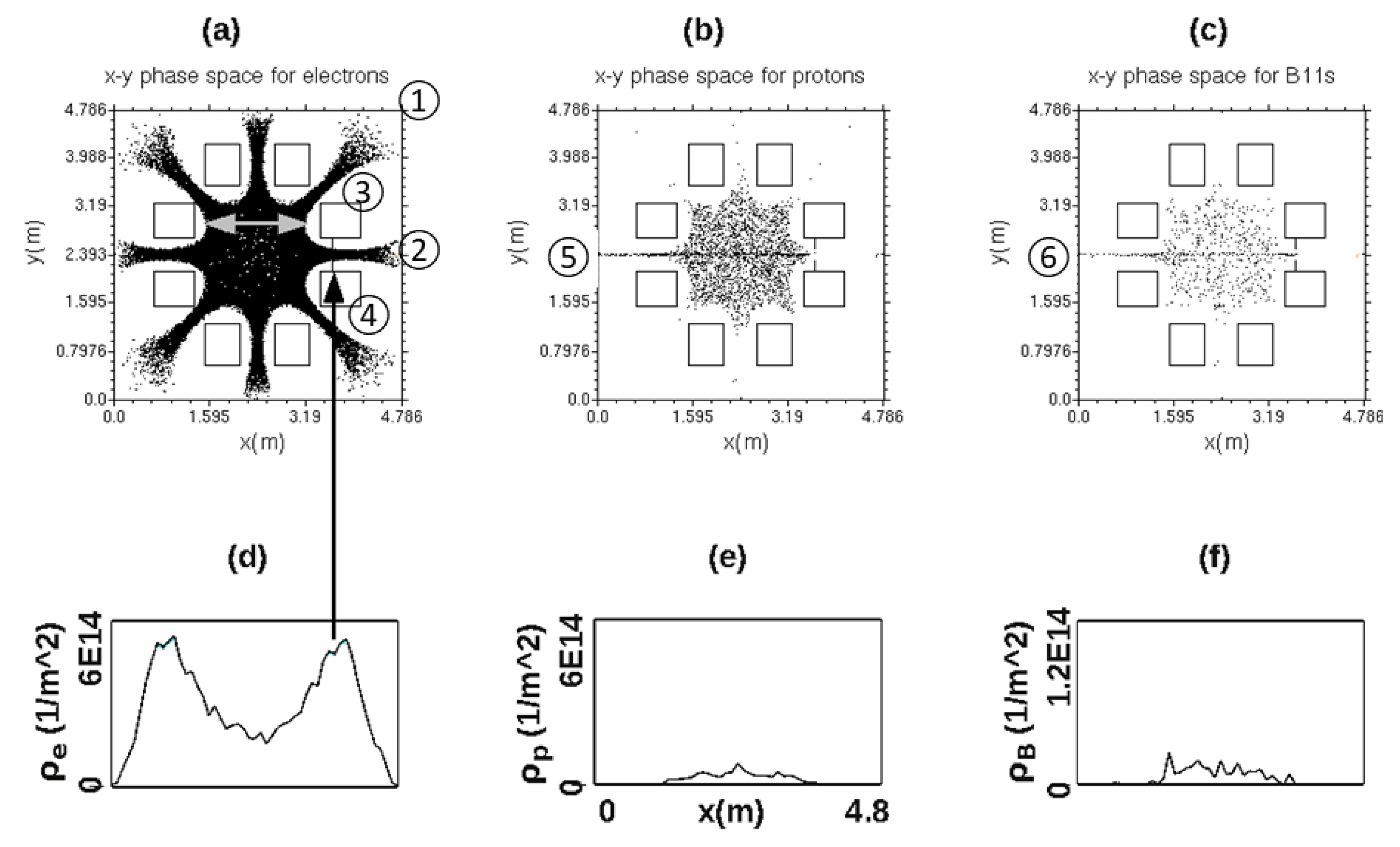
Figure 2.
Diagnostic-displays from simulating a MET6 reactor operating in high-density mode. Individual panels are as follows: (a) 2D map (online magenta = 2.4MV) of electrostatic potential. (b) 3D rendering of magnetic-field iso-surface [17]. (c) 1D section of x-component of applied B-field. (d) 1D central potential extracted from the 2D potential shown above it. (e) 2D map of protons’ (gray) and borons’ (black) locations in velocity-position phase space (f) Vertical (y) component of magnetic field including diamagnetic cancellation of central field.
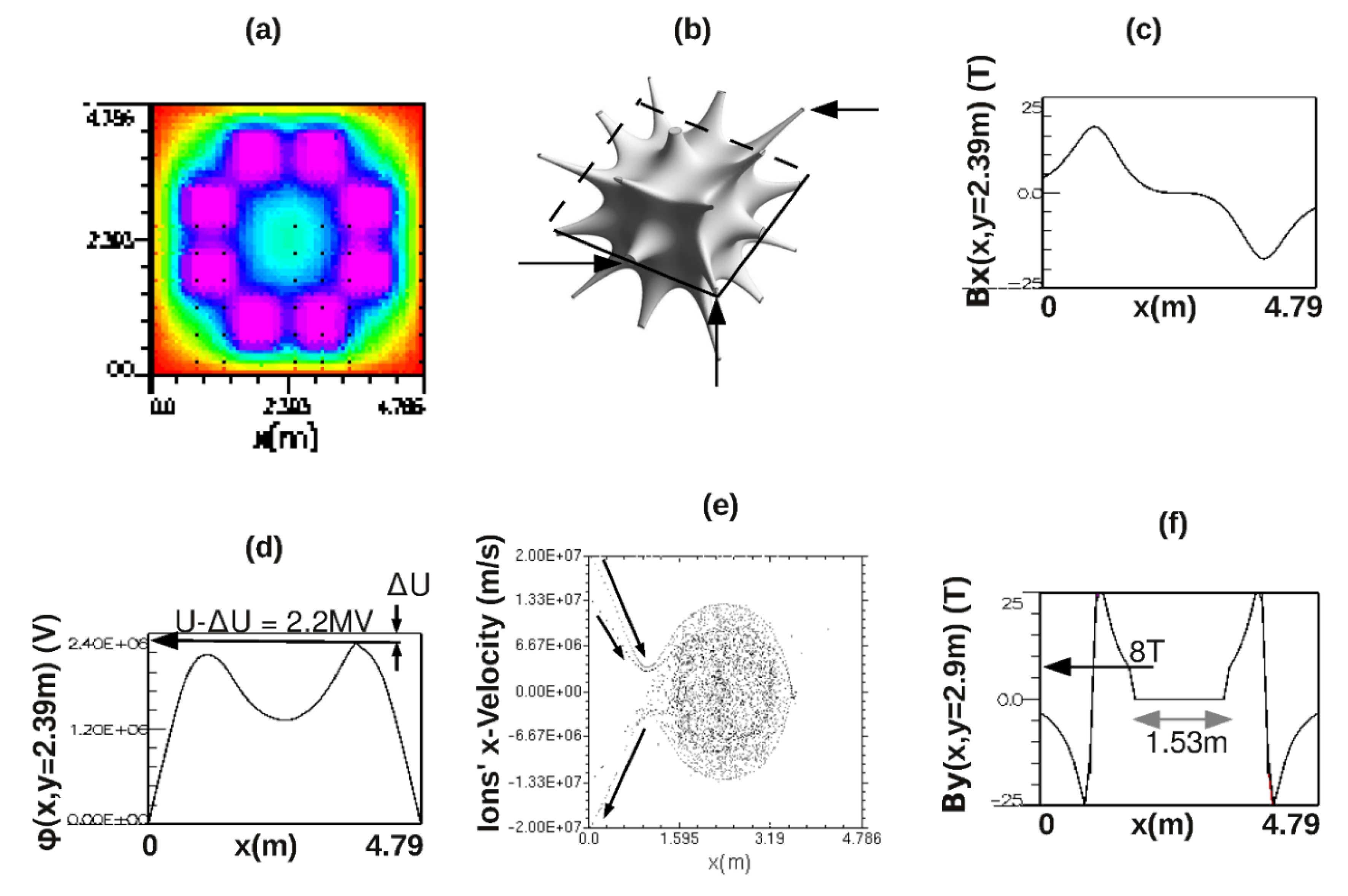
Figure 3.
Thermally averaged fusion reactivities graphed as a function of plasma temperature for various fuel choices. Thick (blue) arrows mark the simulated MET6’s temperature and corresponding pB11 reactivity <σv> = 1.0e-16 /cm3s-1. Graphed data is from ref. [25].
Figure 3.
Thermally averaged fusion reactivities graphed as a function of plasma temperature for various fuel choices. Thick (blue) arrows mark the simulated MET6’s temperature and corresponding pB11 reactivity <σv> = 1.0e-16 /cm3s-1. Graphed data is from ref. [25].
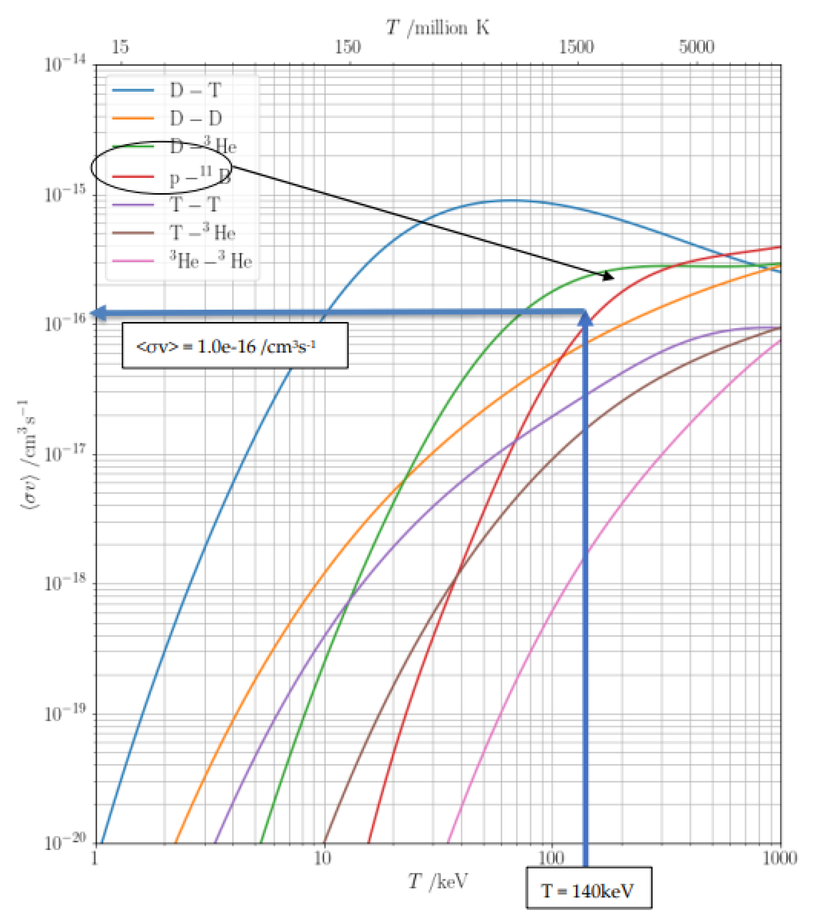
Figure 4.
PIC simulations of MET6 reactor demonstrating electron cooling designed to reduce bremsstrahlung radiation loss. The two panels on the left are simulated with the nominal 15A electron injection current, the same as in the previous figures. The two panels on the right are with 4X higher injection current. The increased injection current produces a deeper potential well and therefore cooler circulating electrons.
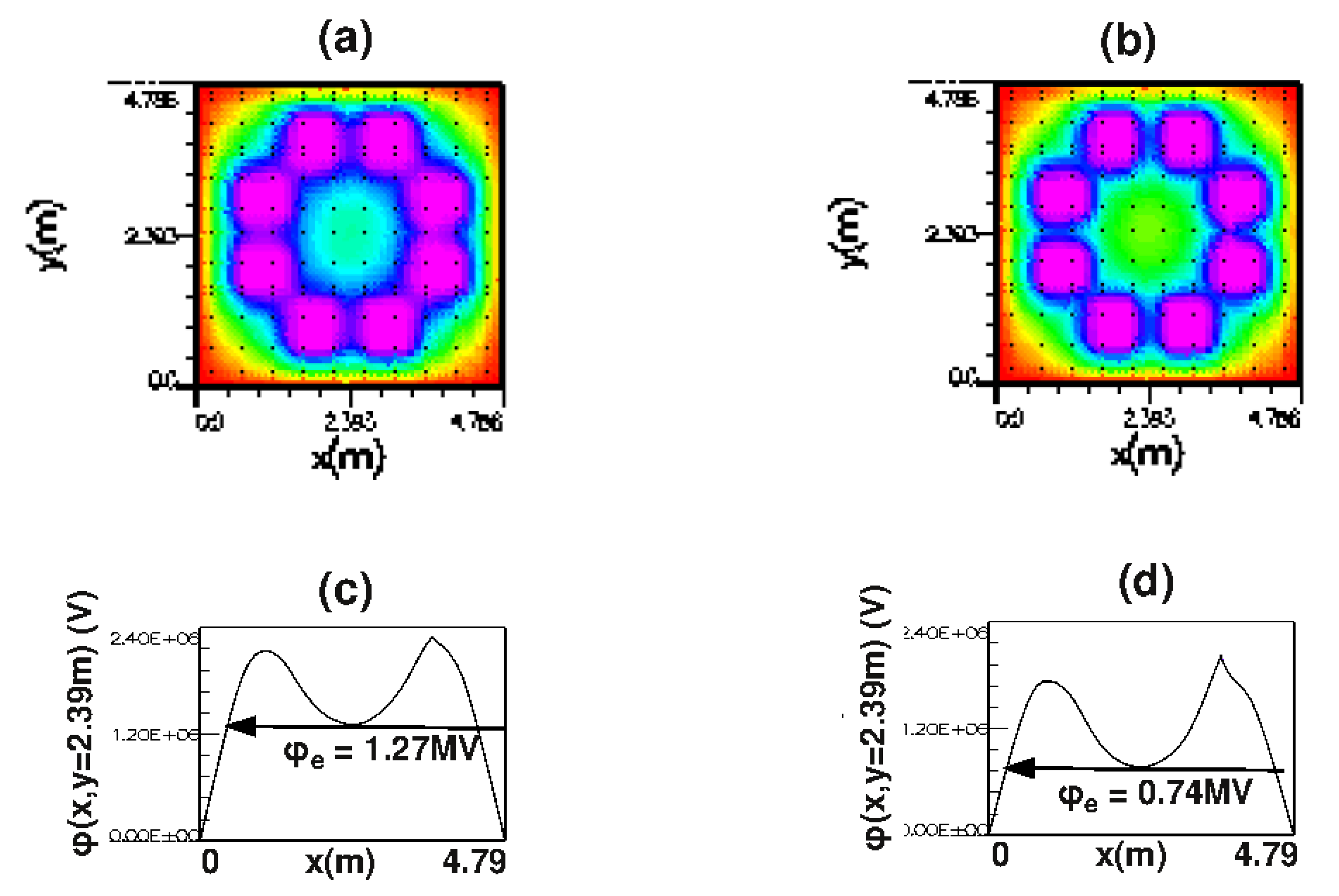

Table 1.
Comparison of Sporer’s HTS reactor with our MET6 reactor.
| Reactor Parameter | HTS ref. [3] | MET6 |
| B-field in anode cusps B (Teslas) | 16 | 18 |
| Applied voltage U (kV) | 500 | 2400 |
| Anode gap spacing b (mm) | 4 | 80 |
| Plasma electron density n (m-3) | 2.9e20 | 1.3e21 |
| Plasma temperature T (keV) | 25 | 140 |
| Coil/cusp radius R (cm) | 83 | 57 |
| Plasma length L (m) | 10 | 5 |
| Fuel species | D+T | p+B11 |
| Power-balance Q | 10 | 1.3 |
Disclaimer/Publisher’s Note: The statements, opinions and data contained in all publications are solely those of the individual author(s) and contributor(s) and not of MDPI and/or the editor(s). MDPI and/or the editor(s) disclaim responsibility for any injury to people or property resulting from any ideas, methods, instructions or products referred to in the content. |
© 2025 by the authors. Licensee MDPI, Basel, Switzerland. This article is an open access article distributed under the terms and conditions of the Creative Commons Attribution (CC BY) license (http://creativecommons.org/licenses/by/4.0/).
Copyright: This open access article is published under a Creative Commons CC BY 4.0 license, which permit the free download, distribution, and reuse, provided that the author and preprint are cited in any reuse.


