Submitted:
21 March 2025
Posted:
21 March 2025
You are already at the latest version
Abstract
Many publications on early house and techno music have the character of documentation and include (auto-)biographical statements from contemporaries of the scene. This literature has led to many statements, hypotheses, and conclusions. Weaknesses of such sources are their selective and subjective nature, and the danger of unclear memories, romanticization and constructive memory. Consequently, a validation through content-based, quantitative music analyses is desirable. For this purpose, the HOuse and Techno music from Germany and AMErica (HOTGAME) corpus was built. Metrics from the field of data quality control show that the corpus is representative and explanatory for house and techno music from Germany and the United States of America between 1984 and 1994. HOTGAME can serve as a reliable source for the analysis of early house and techno music using big data methods, like inferential statistics and machine learning.
Keywords:
audio analysis
; recording studio
; techno music
; house music
; music information retrieval
; acid house
; electronic dance music
; MANOVA
; music analysis
1. Introduction
A lot of literature on house and techno music has a documentation character and contains subjective, (auto-)biographic information rather than scientific examination, like [1,2,3,4,5,6,7,8,9,10,11,12]. For researchers, such sources are appreciated. But it has been criticized that such sources, just like house and techno documentaries, are not scientifically sound. They aim at constructing a certain, pithy narrative, do not reflect critically and from various sides, focus on selective aspects, ignore statements that do not match the desired narrative, focus on feelings rather than facts, and use montages and timelines that imply things that have not been said explicitly [13,14][p. 2][15,16]. Moreover, people tend to unconsciously create false memories when they recount their past, or when they give interviews over and over, referred to as constructive memory [17]. Then, redundancy and repetition can bias collective memory [18]. Clearly, researchers have to reflect critically the narratives that often come from a small group of expert contemporary witnesses [14][p. p. 102][19,20], and it is important to put music analysis in relation to its social space [21][p. 81] and scene [22][p. 16]. Analysis of early house and techno music may be of interest for researchers from the field of history, musicology, digital humanities, cultural studies, media studies, ethnology, economics and marketing. But it requires a high-quality dataset.
The aim of the HOTGAME corpus is to serve as a dataset for the purpose of analyzing early house and techno music based on the music itself, providing additional evidence from a new perspective. The aim of this paper is to test whether the HOTGAME corpus has the necessary quality to allow generalizable conclusions on early house and techno music from Germany and the United States of America.
In the field of data science, the importance of data quality control for scientific research and decision-making has been highlighted [23,24,25]. That is, the generalization of observations from a sample to the general population is only valid if the dataset fulfills certain quality requirements:
- Valid Data
- Few Data Duplicates
- Large Sample Size
- Good Data Balance
- Little Missing Data
- No Gender Bias
- Explanatory Features
- Low Feature Multicollinearity
Following the guidance of [25], the HOTGAME corpus was built according to the three phases collect, assess, improve in the context of early house and techno music. In this paper, the quality of the corpus is evaluated regarding the above-listed requirements. The remainder of this paper is structured as follows: In the Materials section, the analyzed music and the extracted features are described. In the Method section, it is explained how the fulfillment of the requirements was evaluated. The Results and Discussion section summarizes the results and discusses their implications, which culminate in the Conclusion.
2. Materials
HOTGAME, the HOuse and Techno from Germany and AMErica corpus contains information on tracks, which is the recognized term for music pieces of these genres [21,26][p. 2][27][p. 114][28][p. 124]. The purpose of the HOTGAME corpus is to enable the validation of statements on the music scene from the music itself, which requires high-quality data. Here, quality is a matter of the corpus itself, and of features extracted from the music. Statements, the corpus, and the features are explained in this section.
2.1. Statements
Based on documentaries and interviews, many conclusions have been drawn, concerning the relevance of the German reunification [5][pp. 72-73][29][p. 62][30][p. 21][31][p. 216][22][p. 56][6][p. 56][32][p. 26], exchange between different German regions [29][p. 109][22][p. 57 and p. 115][33][p. 472][34][p. 43][32][p. 25], between American metropoles [33][p. 472], and between Detroit and Berlin [33][p. 472][32][pp. 25–26][35][p. 107], and the rivalry between Detroit and Chicago [36][p. 353], between Berlin and Frankfurt [1][p. 9][27][p. 153], and between mainstream and underground techno in Germany [35][p. 107]. With an appropriate dataset, these conclusions and other narratives can be validated from the music itself.
The least common denominator is that house and techno music, their emergence and development were distinct between America and Germany [14][p. 16][33][p. 472 and p. 489][36][p. 346][37][p. 154][38,39][p. 243]. This statement serves as a ground truth: Explanatory features should differ significantly between nations, years, and nation*years.
2.2. Corpus
For the HOTGAME corpus, music was taken from private collections, the university collections, and acquired through second-hand online record and CD stores. This ensured that the data was valid and legal. In [10,11,12,14,22,27,32,35,37,40] German and US-American artists and record labels can be found. The labels served as a starting point to search for the respective artists and other licensed artists, their co-producers, features, and remixers. From these, all licensing record labels were identified. In Germany, 101 dance record labels were identified that were active between 1985 and 1994. In the United States, 91 labels were found that were active between 1984 and 1994. A list of record labels is provided in the repository. Artist names from these labels were collected. House and techno music from these artists were also considered when the music was released on labels from other countries or labels with a larger range of music genres. Based on this data, a representative music corpus was built.
Only house and techno music and their descendants were incorporate. Music considered ancestors of house, such as (Italy) disco, industrial, and Krautrock, was not included. Music clearly assigned to parallel developments, like Electronic Body Music (EBM), Miami bass, electro funk, synth-pop, high-NRG, Neue Deutsche Welle, and new wave, was also ignored. Only music until 1994 was included for two reasons: 1) There is consensus that the mainstream breakthrough of house and techno can be dated back to 1994 [32][p. 45][7][p. 258][33][p. 193], which is why 2) the sheer number of record labels and releases grew too fast to collect a representative sample from 1995 onward (cf. [41][p. 237][33][p. 193][32][p. 45][7][p. 258]).
The HOTGAME corpus consists of CSV-files in two folders germany and usa. A track was assigned to the nation where the producer(s) grew up. Their place of birth and place of residence were not considered. The nationality of the performers was not considered. When a track was remixed, the track was assigned to the nation where the remixer grew up. The filenames consist of artist - title (version) (year).format.csv. The CSV files contain feature vectors that are discussed in the next section.
2.3. Features
In HOTGAME, tracks were stored as lossy compressed audio files with a sample rate of Hz. They were sliced into time frames of 2048 samples, i.e., around 50 ms, with no overlap. The first and last 4 seconds were cropped to remove silence and pure vinyl crackle. From each frame, several audio features were extracted.
There is a consensus that the production process plays the central role in house and techno music [14,26,42][p. 6][21][p. 84], especially the sound design [35][p. 108][43][p. 210] in terms of intensity [14], stereo position [33][p. 142], dynamics [33][p. 142], tempo [14,33,35][p. 102][7][p. 256][43][p. 190] and sound color [14,33][sect. 3.8]. Anylszing house and techno music using the same tools that music producers use in the recording studio when tuning their sound promises to deliver causal and interpretable results. The recording studio analyzers are briefly described in the following sections. A more detailed explanation can be found in [44,45,46]. As the features relate to audio engineering parameters and aspects of sound perception, the sound terminology of [47] is utilized, carefully distinguishing between acoustical and perceptual terms.
2.3.1. Phase Space
Phase space diagrams are point clouds in which the left channel is plotted over the right channel. They serve to monitor volume and stereo position of a mix. Perceptually, these audio aspects relate to loudness, and auditory event angle [48].
2.3.2. Channel Correlation
Channel correlation meters display the Pearson correlation coefficient (P) between the two stereo channels over each time frame. Perceptually, the absolute value of the channel correlation relates to the apparent source width [48]. Phase scope and channel correlation meter are often combined in audio analysis tools [49]. In [46], the combination of phase and channel correlation meter served to tell various hip hop producers apart. In [45], phase scope and channel correlation meter were shown to be orthogonal and explanatory to distinguish different music genres.
2.3.3. Peak
2.3.4. Root Mean Square
2.3.5. Crest Factor
The crest factor is a logarithmic value that describes the relationship between peak and RMS. Sometimes, it is referred to as dynamic range. Acoustically, it describes how impulsive the sound is, which relates to the perception of percussiveness [44]. Music producers consult crest factor meters for example to monitor how much drum sounds stand out of the rest of the mix. Peak, RMS and crest factor meters are utilized in [42,44,51] to analyze aspects of dynamics in mainstream music, electronic dance music, and music mixing in general.
All the above-mentioned features are utilized in the recording studio to analyze aspects of the music mix. In [44,46], they were also extracted from three frequency bands, as music producer usually treat bass (approx. 20–150 Hz), mids (approx. 150– Hz), and highs (approx. 2000– Hz) differently [52][p. 25]. Their balance contributes to the sound color, which is important in house and techno music[14,33][sect. 3.8].
2.3.6. Beats Per Minute
When producing house and techno tracks, the Beats Per Minute (BPM) are set (not monitored), to define the tempo of a song. Concordantly, the BPM are considered important for the definition of and distinction between house and techno music and its various styles [14,35][p. 4][33][p. 102][7][p. 256][43][p. 190]. BPM are extracted from each track, not from each time frame, and not from each frequency region.
This yields 21 features, namely phase, scope, channel correlation, peak, RMS and crest factor for the broadband signal and three different frequency regions, and the BPM.
3. Method
The HOTGAME corpus shall serve as a dataset to study the music, and validate documented statements, narratives, and conclusions through automated content-based audio analysis. Therefore, the corpus has to be representative for the nations and the development over the years. Moreover, the extracted features have to be meaningful descriptors of the considered music. This means that they exhibit significant differences over nation and year. Ideally, the features are mutually independent.
3.1. Corpus
In data quality control, validity and few data duplicates are mostly relevant for material that has been gathered by third parties, like citizen science. As HOTGAME is a first-hand dataset, the validity and few data duplicates are secured, but can be retraced with a look at the dataset and the feature extraction algorithms provided in the repository. To evaluate the appropriateness of the sample size, HOTGAME is compared to other music analysis datasets, and to the size of the house and techno market of the time.
To test for a good data balance and little missing data, the number of track in HOTGAME is compared to the number of dance music labels in Germany and the United States.
3.2. Features
Second, the features are evaluated. Here, a test for feature multicollinearity is applied, using confusion matrices of the features’ mean, median, standard deviation, and skewness values. To test weather the features are explanatory features of the house and techno music of the considered era, a two-way MANOVA is carried out to test whether the features differ significantly over nation, year and nation*year.
4. Results and Discussion
4.1. Corpus
The corpus contains music from 97 German and 85 US-American labels to avoid a bias towards certain labels. This is necessary, as each techno label has its unique sound [35][p. 108]. As various sources agree that in 1995/1996, techno labels existed worldwide [41][p. 237][29][p. 159], the number of labels included in HOTGAME is certainly closer to an all-of than a best-of. As both nations had a similar number of record labels, the HOTGAME corpus also contains an even distribution of German and US-American tracks.
Figure 1 shows the number of active record labels and the number of tracks in the HOTGAME corpus for each year. In Germany (, ) and in the United States (, ), a significant correlation between the number of record labels and tracks can be found, indicating that the HOTGAME corpus represents the development of house and techno releases well. The exponential growth over time is in accordance with the growing market [41][p. 237][29][p. 159].
With almost all labels included, a balance between the two nations, and a correlation between the number of tracks and active record labels, the HOTGAME corpus avoids the dangers of missing data and data imbalance. The small number of female artists in the corpus is in accordance with the low number of releases from female artists on the considered labels, and the low number of female DJs at that time [19][p. 426]. So the gender bias in the dataset is representative for the actual gender bias at that time.
With tracks over the course of 11 years, the early house and techno corpus is comparably large. For example, the corpus in [42] contained tracks over the course of 45 years to analyze the loudness war in mainstream music. In [44], tracks over the course of 5 years have been analyzed to predict which DJ would play which track. [46] analyzed about 350 songs over the course of 20 years to find out whether producers or rappers have a greater influence on the sound in hip hop music. [53] analyzed 55 multi-track recordings to explore the mixing behavior of audio engineers in rock music. One exceptional dataset is the million song dataset, which contains information about one million “western commercial” songs over a period of 90 years [54]. Althoug the corpus is huge, it contains very few early house and techno tracks. Overall, the HOTGAME corpus is large compared to the number of releases during the considered time period.
Overall, the high number of labels, the balance between nations, and the distribution over the years indicate sufficiently large sample size and a good data balance.
4.2. Features
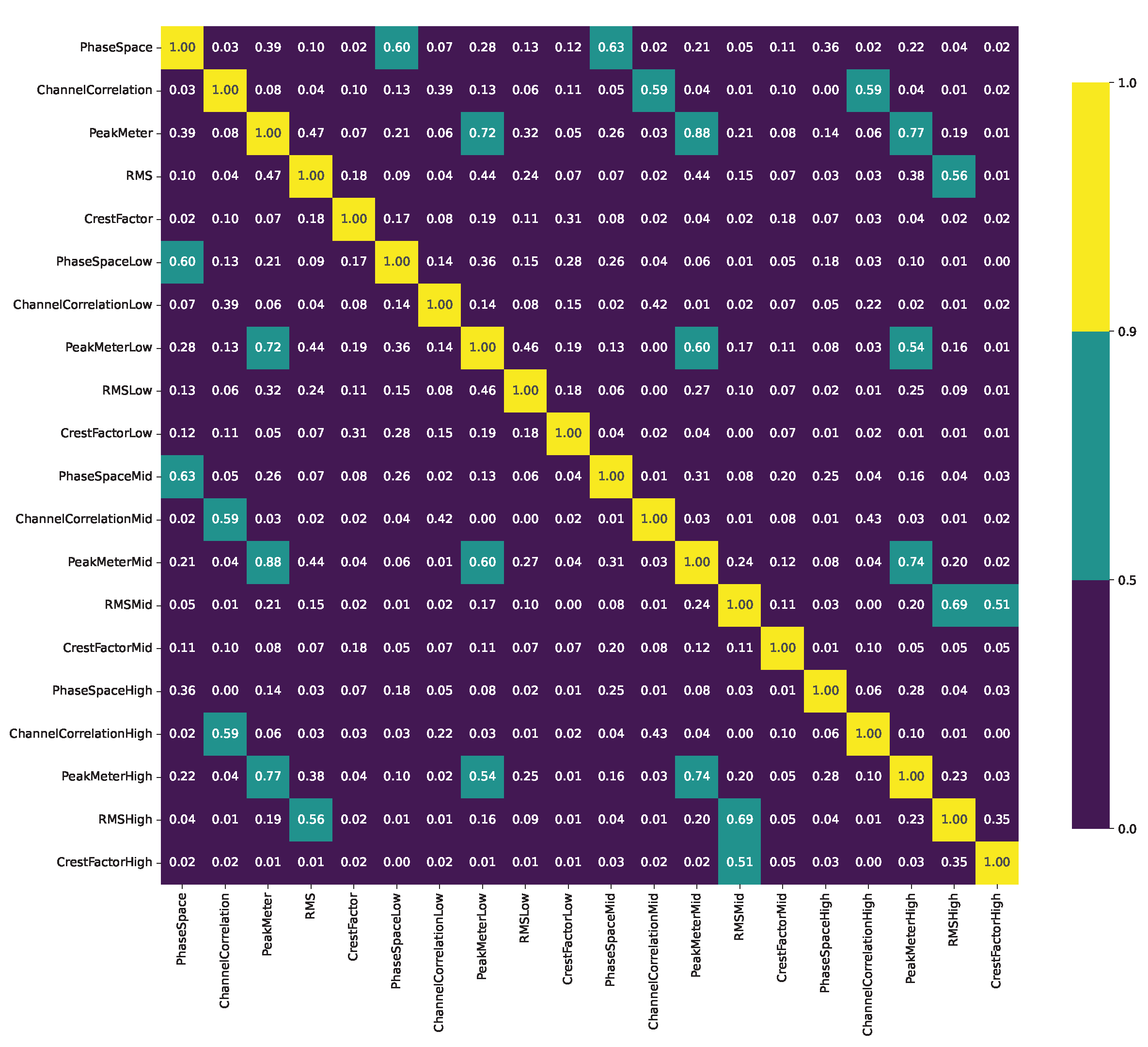
Figure 2 shows a correlation matrix of all features’ median values. Clearly, some features’ median values do not exhibit linear relationships with the others, like CrestFactorHigh and bpm. In contrast, PeakMeter and RMS exhibit a high correlation. This is true for the broadband signal and each frequency region. Both also exhibit a medium to high correlation with the PhaseSpace.
In contrast, the correlation matrix of the mean values, as illustrated in Figure 3, shows almost no high correlations. The only exception is a high correlation between RMShigh and CrestFactorHigh.
A similar picture is provided by the correlation matrix of the standard deviations, as illustrated in Figure 4. Here, almost none of the distributions correlates highly with each other. The only exception is the correlation between PeakMeter and PeakMeterMid.
Lastly, the skewness is compared between all features. The result is illustrated in Figure 5. Here, no high correlations can be found at all. This means that there is not a single pair of features that exhibits the same distribution skewness amongst the music corpus.
Some high correlations between the median values imply the risk multicollinearity, i.e., that the features are not orthogonal to each oter. In big data analyses, redundancy reduction in terms of feature selection or dimensionality reduction is advisable. However, almost no high correlations are found between the features’ mean values, standard deviations, and skewness values, indicating fair independence of the features and variation among the distributions.
The recording studio features were already selected because the literature indicates that the sound parameters that they quantify are highly relevant for house and techno music [14,21,26,33,35,42,43]. Two-way MANOVA reveals if the features are indeed explanatory in terms of capturing the difference between nation, year and nation*year. This is expected, as the literature suggests that house and techno music evolved differently in Germany and the United States of America. The result is that the extracted features differ significantly between nation ( Wilk’s , ), year ( Wilk’s , ), and nation*year ( Wilk’s , ). That means the extracted features seem explanatory for early house and techno music and can be utilized for further exploration and analyses of the HOTGAME corpus.
It has to be kept in mind that many house and techno tracks have never been released [43][p. 185]. And clearly, the music corpus does not reveal which tracks have been played a lot in night clubs, and which had no impact. Naturally, US-American music has been sold and played in Germany and vice versa. These things have to be kept in mind when analyzing the HOTGAME data.
5. Conclusions
This paper introduced HOTGAME, a corpus of early HOuse and Techno music from Germany and AMErica. Putting the dataset in relation with the existing literature, the market, and other datasets indicated that the source material and the extracted features are representative and explanatory for the house and techno music of the considered time and nations. The gender bias is in accordance with the general house and techno market. The features are not perfectly independent and may require redundancy reduction. Then, the path is clear for the content-based exploration and examination of house and techno music. Researchers can add even more tracks to the dataset or create their own dataset. The feature extraction algorithm is provided in the repository and the presented quality control methods provide metrics for the corpus validity.
Funding
This research received no external funding.
Data Availability Statement
The HOTGAME corpus and lists of retrieved and missing labels are available on Zenodo under https:doi.org/10.5281/zenodo.14958956 (submitted to the Zenodo curators, not publicly available yet). The feature extraction and statistical analyses are available on Github under https://github.com/ifsm/HOTGAME-feature-extraction.
Acknowledgments
I thank my students who helped me clean and double-check the data.
Conflicts of Interest
The author declares no conflicts of interest.
Abbreviations
The following abbreviations are used in this manuscript:
| BPM | Beats Per Minute |
| CSV | Comma Separated Value |
| HOTGAME | House and Techno music from Germany and AMErica |
| MANOVA | Multivariate Analysis Of VAriance |
| P | Pearson’s correlation coefficient |
| p | probability value |
| RMS | Root Mean Square |
References
- Denk, F.; von Thülen, S. Der Klang der Familie. Berlin, Techno und die Wende, 6 ed.; Suhrkamp Verlag: Berlin, 2022. [Google Scholar]
- Franke, M. ; X-Teknokore. Rave is Pain; EHM: Dresden, 2024. [Google Scholar]
- Karnes, K.C. A German DJ, Postmodern Dreams, and the Ambivalent Politics of East–West Exchange at the First Exhibition of Approximate Art in Riga, April 1987. Arts 2024, 13, article number 88. [Google Scholar] [CrossRef]
- Hidalgo, D.A. Dance Music Spaces; Lexington Books: Lanham, 2022. [Google Scholar]
- Reige, M. Deep in Techno. Die ganze Geschichte des Movements; Schwarzkopf & Schwarzkopf, 2000.
- Coers, M.M. Friede Freude Eierkuchen. Die Technoszene; C. H. Beck: München, 2000. [Google Scholar]
- Laarmann, J. Fuck the depression – We are alive! In Kursbuch JugendKultur; SPoKK., Ed.; Bollmann: Mannheim, 1997; pp. 256–272. [Google Scholar]
- Westbam. Die Macht der Nacht; Ullstein: Berlin, 2016. [Google Scholar]
- Phillips, D. Superstar DJs here we go! The rise and fall of the superstar DJ; Ebury Press: London, 2009. [Google Scholar]
- Anz, P.; Walder, P. Techno; Ricco Bilger: Zürich, 1995. [Google Scholar]
- Sicko, D. Techno Rebels, 2 ed.; Wayne State University Press: Detroit, MI, 2010. [Google Scholar]
- Anthony, W. Class of 88; Virgin Books: London, 1998. [Google Scholar]
- Keilbach, J. We Call It Techno! Zeitzeugen und die filmischeKonstruktion von Technogeschichte. In techno studies. Ästhetik und Geschichte Elektronischer Tanzmusik; Feser, K., Pasdzierny, M., Eds.; b-books: Berlin, 2016. [Google Scholar]
- Volkwein, B. What’s Techno. Geschichte, Diskurse & musikalische Gestalt elektronischer Unterhaltungsmusik; epOs Music: Osnabrück, 2003; https://www.epos.uni-osnabrueck.de/books/v/volb03/pages/index.htm. [Google Scholar]
- Thompson, P. An empirical study into the learning practices and enculturation of DJs,turntablists, hip hop and dance music producers. Journal of Music, Technology & Education 2012, 5, 43–58. [Google Scholar] [CrossRef]
- Pasdzierny, M. „Das Nachkriegstrauma abgetanzt“? Techno und die deutsche Zeitgeschichte. In Techno Studies. Ästhetik und Geschichte elektronischer Tanzmusik; Feser, K., Pasdzierny, M., Eds.; b_books: Berlin, 2016; pp. 105–119. [Google Scholar]
- Wagoner, B. Constructive Memory. In The Palgrave Encyclopedia of the Possible; Glaveanu, V.P., Ed.; Springer International Publishing: Cham, 2020; pp. 1–6. [Google Scholar] [CrossRef]
- Orianne, J.F.; Eustache, F. Collective memory: between individual systems of consciousness and social systems. Frontiers in Psychology 2023, 14. [Google Scholar] [CrossRef]
- Pasdzierny, M. Transatlantic Techno Myths: The 1994 Arica Eclipse Rave as an Example of the History and Historiography of Electronic Dance Music between Chile and Germany. Twentieth-Century Music 2020, 17, 419–433. [Google Scholar] [CrossRef]
- Lothwesen, K.S. Methodische Aspekte der musikalischen Analysevon Techno. In Erkenntniszuwachs durch Analyse. Populäre Musik auf dem Prüfstand; Rösing, H., Phleps, T., Eds.; Coda: Baden Baden, 1999; pp. 70–89. [Google Scholar]
- Hawkins, S. Feel the beat come down: house music as rhetoric. In Analyzing Popular Music; Moore, A.F., Ed.; Cambridge University Press: Cambridge, 2009; chapter 5, pp. 80–102. [Google Scholar] [CrossRef]
- Meyer, E. Die Techno-Szene; Leske + Budrich: Opladen, 2000. [Google Scholar]
- Li, N.; Qi, Y.; Li, C.; Zhao, Z. Active Learning for Data Quality Control: A Survey. J. Data and Information Quality 2024, 16. [Google Scholar] [CrossRef]
- Gudivada, V.N.; Apon, A.; Ding, J. Data Quality Considerations for Big Data andMachine Learning: Going Beyond Data Cleaning andTransformations. International Journal on Advances in Software 2017, 10, 1–10. [Google Scholar]
- Serra, F.; Peralta, V.; Marotta, A.; Marcel, P. Use of Context in Data Quality Management: A Systematic Literature Review. J. Data and Information Quality 2024, 16. [Google Scholar] [CrossRef]
- Schaubruch, J. »Von Menschen, Maschinen und dem Minimalen«. Musikanalytische Überlegungen zum Techno-Projekt The Brandt Brauer Frick Ensemble. SAMPLES. Open Access Journal for Popular Music Studies 2016, 14. 27 pages. [Google Scholar]
- Kühn, J.M. Die Wirtschaft der Techno-Szene; Springer: Wiesbaden, 2017. [Google Scholar] [CrossRef]
- Papenburg, J.G. Produktion. In Handbuch Popkultur; Hecken, T., Kleiner, M.S., Eds.; J. B. Metzler: Stuttgart, 2017; chapter 17, pp. 123–128. [Google Scholar]
- Henkel, O.; Wolff, K. Berlin Underground. Techno und HipHop zwischen Mythos und Ausverkauf; FAB Verlag: Berlin, 1996. [Google Scholar]
- Anz, P.; Meyer, A. Die Geschichte von Techno. In Techno; Anz, P., Walder, P., Eds.; Ricco Bilger: Zürich, 1995; pp. 8–21. [Google Scholar]
- Schiller, M. The popularization of electronic dance music. In Perspectives on German Popular Music; Ahlers, M., Jacke, C., Eds.; Routledge: New York, 2017; pp. 217–222. [Google Scholar]
- Lemm, N. Techno- und Ravekultur als posttraditionale Vergemeinschaftungvon Jugendlichen; Diplomica Verlag: Hamburg, 2014. [Google Scholar]
- Hemming, J. Methoden der Erforschung populärer Musik; Springer: Wiesbaden, 2016. [Google Scholar]
- Oczenaschek, P. Technomusik, Festivals und die zugehörigen Marken; Diplomica: Hamburg, 2012. [Google Scholar]
- Kaul, T. Techno. In Handbuch Popkultur; Hecken, T.; Kleiner, M.S., Eds.; J. B. Metzler, 2017; pp. 106–110.
- Brewster, B.; Broughton, F. Last Night a DJ Saved My Life. The History of the Disc Jockey; Headline: London, 1999. [Google Scholar]
- Nye, S. Minimal Understandings: The Berlin Decade, TheMinimal Continuum, and Debates on the Legacy ofGerman Techno. Journal of Popular Music Studies 2013, 25, 154–184. [Google Scholar] [CrossRef]
- Meueler, C. Auf Montage im Techno-Land. In Kursbuch JugendKultur; SPoKK., Ed.; Bollmann: Mannheim, 1997; pp. 243–255. [Google Scholar]
- Kaul, T. Electronic Body Music. In Handbuch Popkultur; Hecken, T., Kleiner, M.S., Eds.; J. B. Metzler: Stuttgart, 2017; chapter 17, pp. 102–105. [Google Scholar]
- Schiller, M. From soundtrack of the unification to the celebration of Germanness. In Perspectives on German Popular Music; Ahlers, M., Jacke, C., Eds.; Routledge: New York, 2017; pp. 111–115. [Google Scholar]
- Fehlmann, M. Das Technogeschäft. In Techno; Ricco Bilger: Zürich, 1995; pp. 234–239. [Google Scholar]
- Emmanuel, D.; Damien, T. About dynamic processing in mainstream music. Journal of the Audio Engineering Society 2014, 62, 42–55, [https://aes2.org/publications/elibrary-page/?id=17085]. [Google Scholar]
- Jarrentrup, A. Das Mach-Werk. Zur Produktion, Ästhetik und Wirkung von Techno-Musik. In Techno-Soziologie. Erkundungen einer Jugendkultur; Leske + Budrich: Opladen, 2001; pp. 185–210. [Google Scholar]
- Ziemer, T.; Kiattipadungkul, P.; Karuchit, T. Acoustic features from the recording studio for Music Information Retrieval Tasks. Proceedings of Meetings on Acoustics 2020, 42, 035004. [Google Scholar] [CrossRef]
- Ziemer, T. Goniometers are a Powerful Acoustic Feature for Music Information Retrieval Tasks. In Proceedings of the DAGA 2023 – 49. Jahrestagung für Akustik, Hamburg, Germany, 03 2023; pp. 934–937.
- Ziemer, T.; Kudakov, N.; Reuter, C. Producer vs. Rapper: Who Dominates the Hip Hop Sound? Journal of the Audio Engineering Society 2024, 73, 54–62. [Google Scholar] [CrossRef]
- Ziemer, T. Sound Terminology in Sonification. J. Audio Eng. Soc 2024, 72, 274–289. [Google Scholar] [CrossRef]
- Ziemer, T. Source Width in Music Production. Methods in Stereo, Ambisonics, and Wave Field Synthesis. In Studies in Musical Acoustics and Psychoacoustics; Schneider, A., Ed.; Springer International Publishing: Cham, 2017; pp. 299–340. [Google Scholar] [CrossRef]
- Stirnat, C.; Ziemer, T. Spaciousness in Music: The Tonmeister’s Intention and the Listener’s Perception. In Proceedings of the KLG 2017. klingt gut! 2017 – international Symposium on Sound, Hamburg, 06 2017; pp. 42–51. [CrossRef]
- Rumsey, F.; McCormick, T. Sound and Recording, 6 ed.; Focal Press: Burlington, MA, 2009. [Google Scholar]
- de Man, B.; Leonard, B.; King, R.; Reiss, J.D. An Analysis and Evaluation of Audio Features for Multitrack Music Mixtures. In Proceedings of the 15th Conference ofthe International Society for Music Information Retrieval, Taipei, Taiwan, 2014; pp. 137–142.
- Owsinski, B. The Mixing Engineer’s Handbook; Thomson Course Technology PTR: Boston, MA, 2006. [Google Scholar]
- Deruty, E.; Pachet, F.; Roy, P. Human–Made Rock Mixes Feature Tight RelationsBetween Spectrum and Loudness. J. Audio Eng. Soc. 2014, 62, 643–653. [Google Scholar] [CrossRef]
- Bertin-Mahieux, T.; Ellis, D.P.; Whitman, B.; Lamere, P. The Million Songs Dataset. In Proceedings of the 12th International Society for Music Information Retrieval Conference, Miami, FL, USA, 10 2011; pp. 591–596.
Figure 1.
Bar diagrams showing the number of record labels and tracks in our corpus for Germany (left) and USA (right).
Figure 1.
Bar diagrams showing the number of record labels and tracks in our corpus for Germany (left) and USA (right).
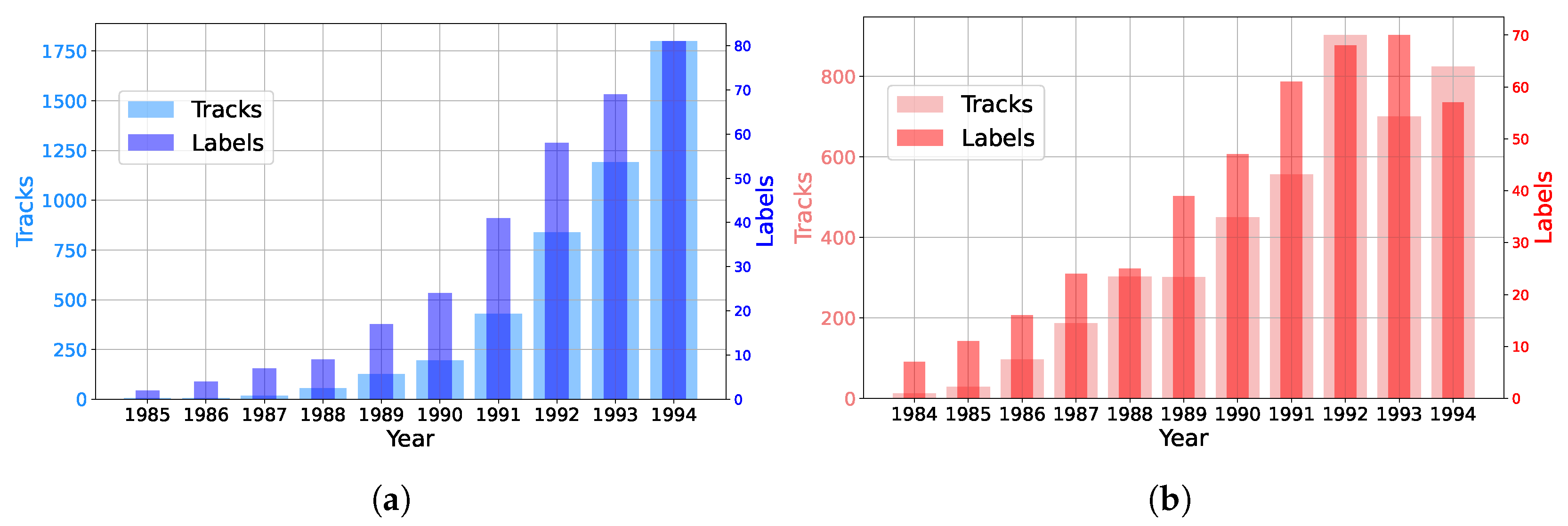
Figure 2.
Pearson’s correlation coefficients P between the median values of all extracted features with a high correlation () in yellow, a moderate correlation () in cyan and a low correlation () in blue.
Figure 2.
Pearson’s correlation coefficients P between the median values of all extracted features with a high correlation () in yellow, a moderate correlation () in cyan and a low correlation () in blue.
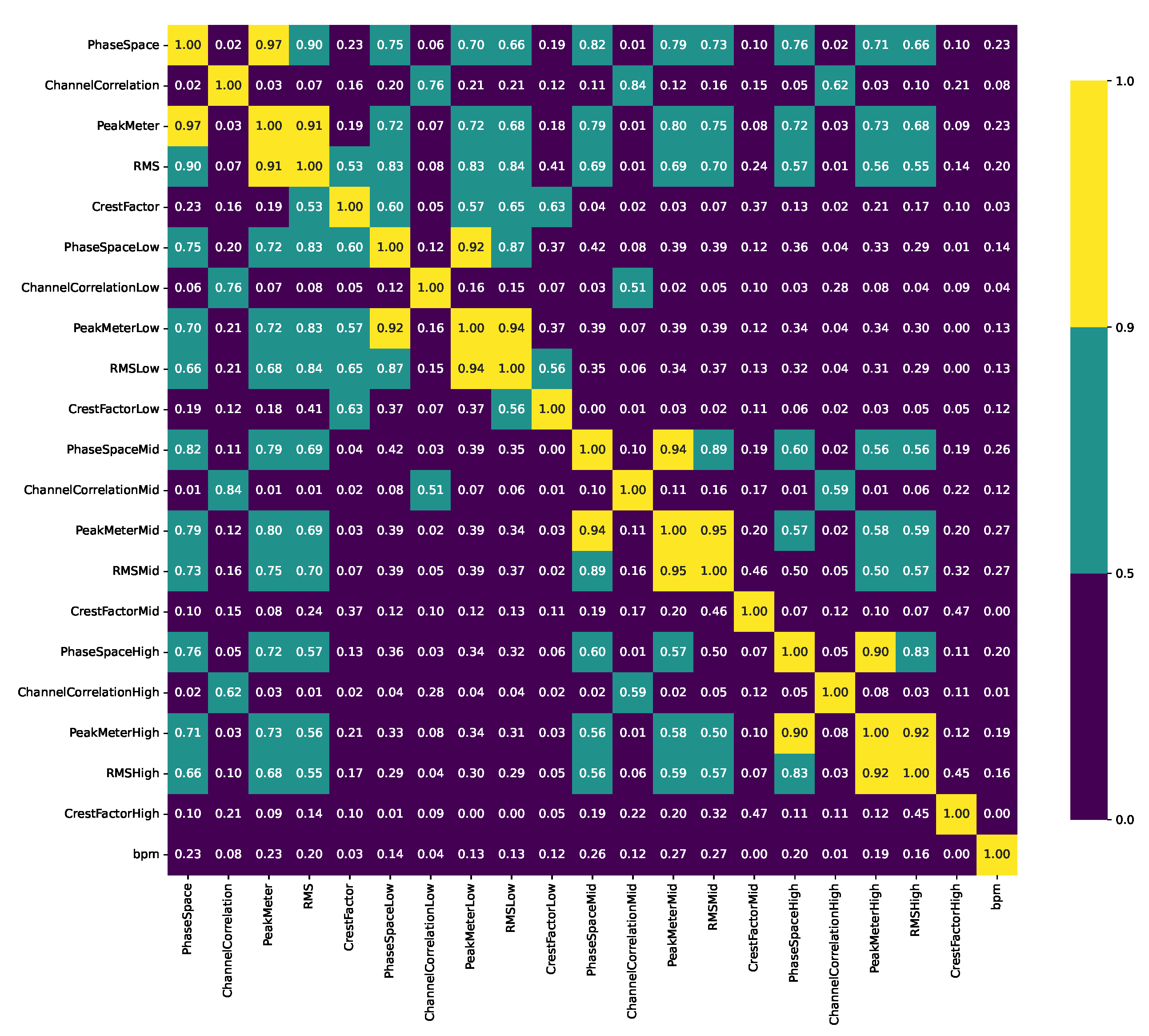
Figure 3.
Pearson’s correlation coefficients P between the mean values of all extracted features with a high correlation () in yellow, a moderate correlation () in cyan and a low correlation () in blue.
Figure 3.
Pearson’s correlation coefficients P between the mean values of all extracted features with a high correlation () in yellow, a moderate correlation () in cyan and a low correlation () in blue.
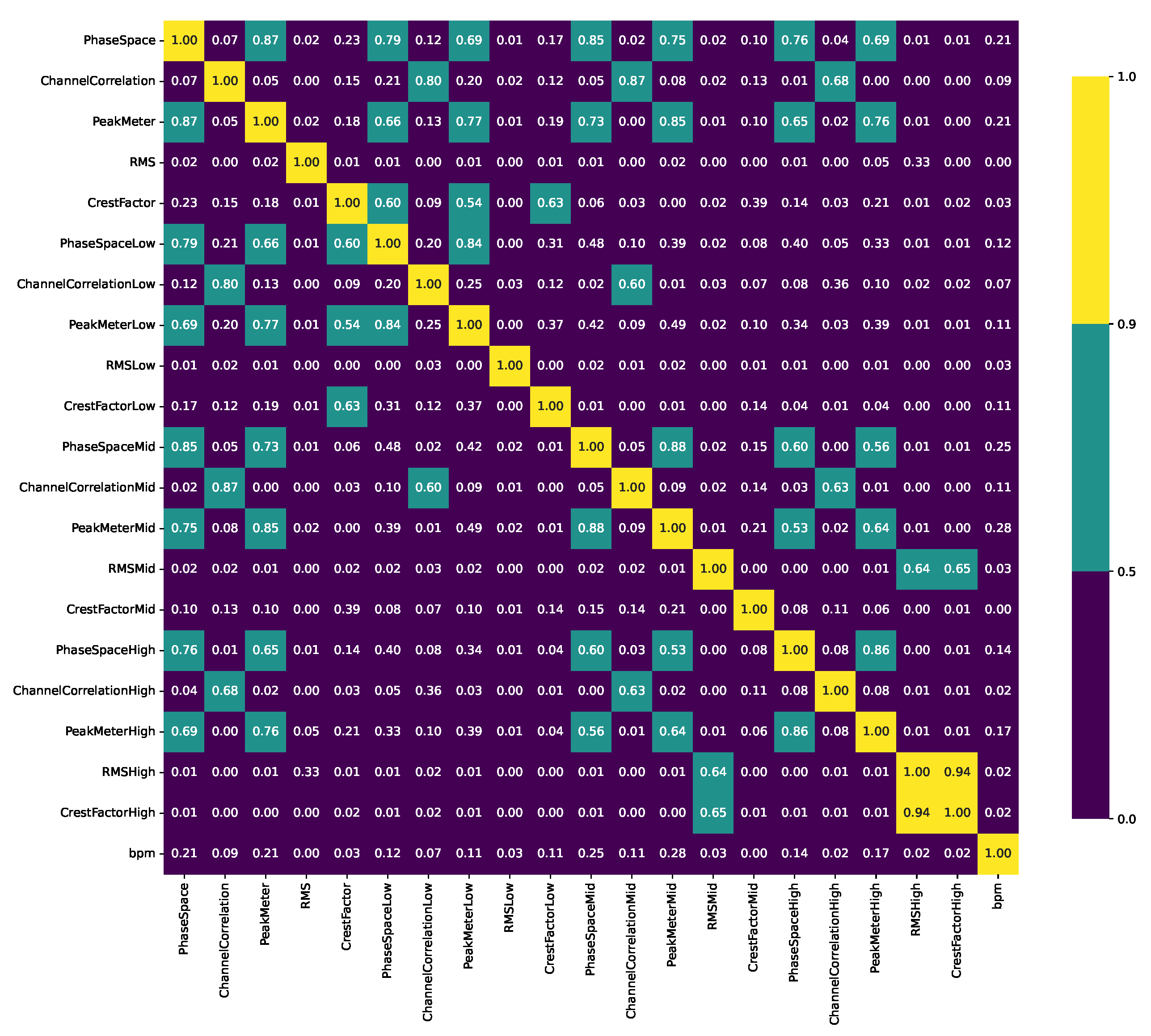
Figure 4.
Pearson’s correlation coefficients P between the standard deviation values of all extracted features with a high correlation () in yellow, a moderate correlation () in cyan and a low correlation () in blue.
Figure 4.
Pearson’s correlation coefficients P between the standard deviation values of all extracted features with a high correlation () in yellow, a moderate correlation () in cyan and a low correlation () in blue.
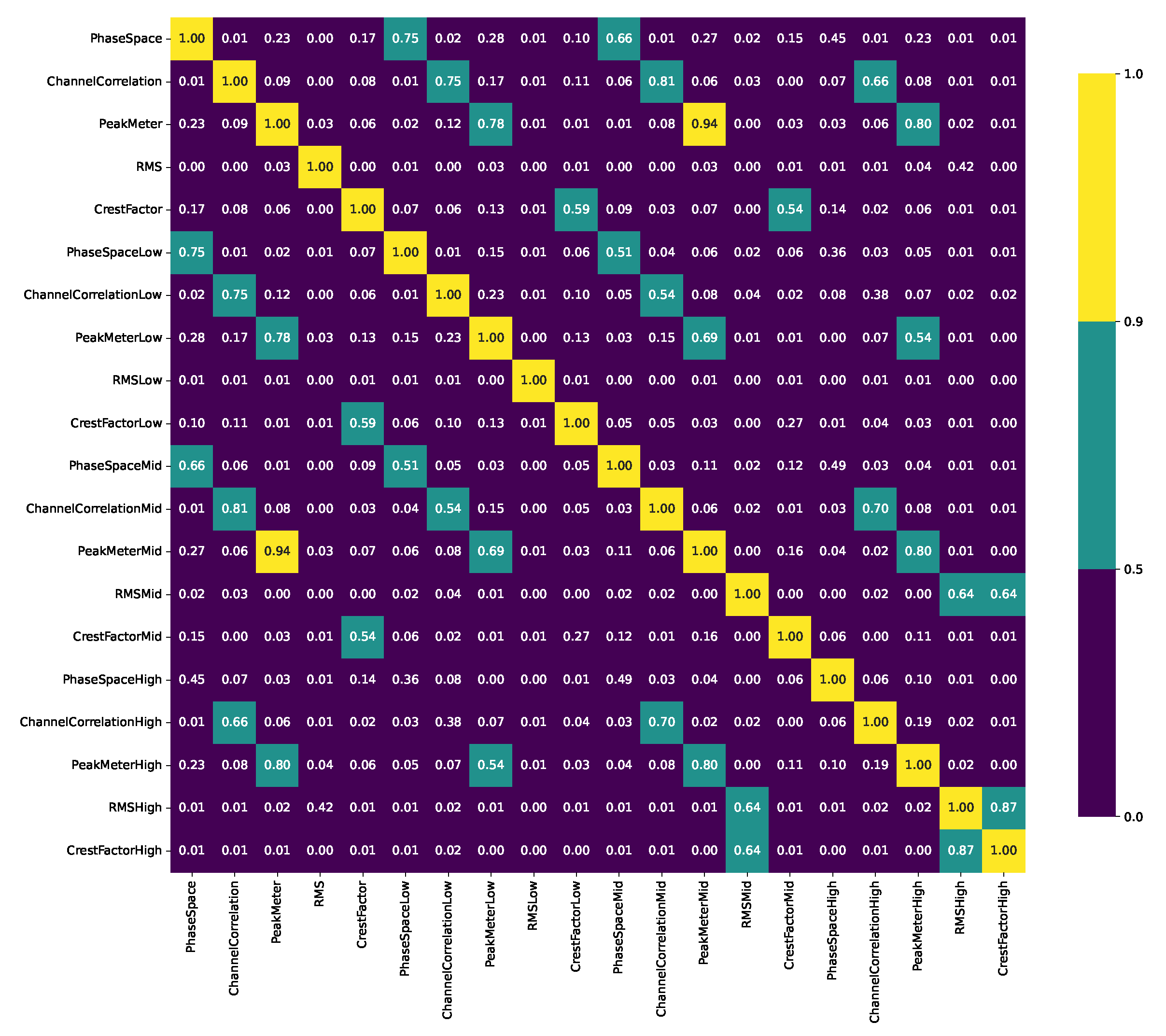
Figure 5.
Pearson’s correlation coefficients P between the skewness of all extracted features with a high correlation () in yellow, a moderate correlation () in cyan and a low correlation () in blue.
Figure 5.
Pearson’s correlation coefficients P between the skewness of all extracted features with a high correlation () in yellow, a moderate correlation () in cyan and a low correlation () in blue.
Disclaimer/Publisher’s Note: The statements, opinions and data contained in all publications are solely those of the individual author(s) and contributor(s) and not of MDPI and/or the editor(s). MDPI and/or the editor(s) disclaim responsibility for any injury to people or property resulting from any ideas, methods, instructions or products referred to in the content. |
© 2025 by the authors. Licensee MDPI, Basel, Switzerland. This article is an open access article distributed under the terms and conditions of the Creative Commons Attribution (CC BY) license (http://creativecommons.org/licenses/by/4.0/).
Copyright: This open access article is published under a Creative Commons CC BY 4.0 license, which permit the free download, distribution, and reuse, provided that the author and preprint are cited in any reuse.


