Submitted:
19 March 2025
Posted:
20 March 2025
You are already at the latest version
Abstract
System suitability testing of chromatography is an indispensable procedure in pharmaceutical analysis, and must comply with rules in related pharmacopoeias. An inverse Fourier transform algorithm is developed to accurately evaluate chromatographic features versus a standard Gaussian peak shape. The regular chromatogram is considered as a pseudo-frequency spectrum and can be converted to a nominal time signal by inverse Fourier transformation. The system suitability parameters of peak width, theoretical plate number, tailing factor and noise testing were evaluated by linear regressions directly and compared with the compendial rules. This novel method is simple, accurate, robust, reliable and efficient for evaluation of chromatographic peak features.
Keywords:
chromatographic peak feature
; system suitability
; pharmaceutical analysis
; inverse Fourier transform
; Gaussian and distortion peaks
1. Introduction
Pharmaceutical quality controls are closely related to therapeutical effects and public health. Various chromatographs are essential and principal equipment in analytical and research laboratories of pharmaceutical industries. System suitability criteria of chromatography ensure accuracy and reliability of chromatographic analysis. The important performance evaluations include peak width, theoretical plate number, tailing factor, and resolution if more than one analytical component in the chromatogram. Highly pure standard substances usually are used in calibrations of chromatographic systems, and they must display good performance to meet the analytical criteria quantitatively and qualitatively. Their chromatographic peak shape should be outstandingly good and distinguishable with little interferences. The ideal chromatographic peak shape was supposed to be a Gaussian profile [1]. This famous theorem withstands for more than eighty years and testified by modern chromatography and state-of-the-art developments in chromatographic column chemistry [2,3,4,5,6,7,8,9,10,11,12,13,14,15].
A regular chromatographic Gaussian peak can be written as a function of elution time t [2] (pp.217-224):
where A is its intensity, tR is its retention time and Wh is full width at half maximum (FWHM) of the peak. In this work, we study system suitability parameters related to the chromatographic peak features: peak width, theoretical plate numbers, and tailing (or symmetric) factor. It is mandatory to achieve a good peak shape with high plate number in pharmaceutical analysis. According to the current harmonized pharmacopeia monograph [16] in US pharmacopoeia (USP), European Pharmacopoeia and Japan Pharmacopoeia, plate number N should be calculated as:
G(t – tR) = A exp(– 4ln2[(t – tR)/Wh]2),
N = 5.54 (tR/Wh)2.
Since the system suitability test are routinely performed by higher sampling rates, retention time tR of a peak generally can be precisely determined.
Markevich and Gertner compared five different methods to calculate FWHM for Gaussian or near Gaussian profiles in 1989 [17]. The direct measurement of the FWHM is the most in use [16,17]. The second moment (variance) is also used to compute FWHM of a chromatographic peak if the peak profile is exactly known [17]. However, chromatographic noises can affect all of these current methods. Taking a Gaussian profile as a reference (Gaussian paragon), we developed an inverse Fourier transform (FT) algorithm to linearly evaluate FWHM as well as plate number of a chromatographic peak regardless of its real shape with highly denoising capability.
2. Fourier Transform in Chromatography
Despite the fact that the individual components are analyzed regarding their retention times in the column chromatography, the chromatogram actually is a chart recording separations of individual components, similar to a spectrum in spectroscopy. FT algorithm had been introduced to chromatography more than five decades, mainly for peak sharpness and noise suppression [18]. The signal truncations in FT induce Gibbs effect (side-lobes) to the spectral peaks and should be apodized by a proper window function [18]. Therefore, the recovered chromatographic peaks by FT are not genuine ones. Wahab and his colleagues recently initiated several novel approaches to evaluate total chromatographic peak shape rationally matching a Gaussian profile (for example above 80% peak height) [19,20,21]. They further used inverse FT algorithms to sharpen chromatographic peaks and deconvolute highly overlapped peaks when the peak shape tailing was determined [22]. Alternatively, we use inverse FT to measure peak widths and plate numbers of any chromatographic peak versus a Gaussian paragon as long as they are yielded at the same sampling rate.
If a signal f(t) is a function of time t, its FT spectrum F(υ) in frequency domain υ (angular frequency ω = 2πν) is commonly written as [18,23]:
where i = √–1 and exponential function exp(–i2πνt) is the kernel of FT. The inverse FT of F(ν) is defined to be:
We presume that a chromatogram based on the retention time is equivalent to a spectrum in frequency. Thus, the inverse FT can be performed for the chromatogram peaks. For a Gaussian function G(t – tR) = A exp[–απ(t – tR)2], its inverse FT should be [23]:
where t’ is a nominal time in above inverse FT to distinguish retention time t routinely used in chromatography. The retention time t represents a “location” in a chromatogram, corresponding to frequency ν in spectroscopy. As per Equation (1), απ = 4ln2/Wh2. Following Euler’s relation exp(–ix) = cos(xt) – i sin(xt) [18], the inverse FT of the Gaussian peak G(t – tR) is:
The function g(t’) in the nominal time domain is a sinusoidal signal with real cos(tR t’) and imaginary sin(tR t’), which are a Hilbert transform pair in Fourier analysis [24]. Hilbert transform provides a shortcut to extract the wave envelope because absolute value of a complex function |x + iy| = and cos2(tR t’) + sin2(tR t’) = 1:
Taking natural logarithm to both sides of Equation (7),
where KG = π2Wh2/4ln2, Gaussian slope versus nominal (t’)2, and ln[M0] is its intercept of the linear regression (zeroth moment M0 = Gaussian peak area AWh.).
A genuine Gaussian peak of liquid chromatography was simulated in Figure 1(a) by distributing 512 data points from 220 to 271.1 seconds (sampling rate = 10 Hz). We set retention time tR = 240 seconds, FWHM Wh = 5 seconds and peak height A0 = 200 mAU. Its USP plate number = 5.54(240/5)2 = 12764. When applying inverse cosine FT versus nominal t’ lasting from 0 to 0.12 seconds, the Gaussian peak converted to a sinusoidal cos(tR t’) (pink wave) with a Gaussian envelope (dash brown line) in Figure 1(a). A wellbeing outcome in Figure 1(a) is that the inverse cosine FT at nominal t’ = 0 equals to zeroth moment M0 = peak area (AWh) from Equation (8). We need a distinctive feature of the Gaussian shape to compare with the other non-Gaussian shapes. This feature is the Gaussian slope KG in Equation (8). According to the algorithm of Equation (6), we should use both inverse cosine FT and inverse sine FT to extract the envelope |g(t’)|, and then implement linear regression on it natural logarithm ln|g(t’)| versus nominal (t’)2 (0 – 0.0144 s2). Figure 1(b) is a perfect linear regression (R2 ≡ 1) on the Gaussian envelope of Figure 1(a). Its slope kG (= π2Wh2/4ln2) only relates to the peak width of the Gaussian peak.
Any commercial FT software will be suitable to evaluate the Gaussian envelope if the users have initiative to input frequency and time ranges. Because only a few hundreds of data points were involved in the system suitability testing, it is very easy to implement the inverse FT in Excel program as shown in Section S1 of “Supporting Information”.
3. Peak Width Evaluations
In the following simulation studies for non-Gaussian peak width evaluations, we always take sampling rate 10 Hz because this rate (or higher) is sufficient to capture FWHMs around 5 seconds. Meanwhile, the inverse FT was performed with 512 data points.
3.1. Symmetric Peaks
Absolutely symmetric peaks are seldom seen in chromatography. However, it is helpful to study non-Gaussian symmetric shapes first, and understand how to compare non-Gaussian peaks to a Gaussian paragon. One outstanding symmetry is centered Voigt shape. Theoretically, A Voigt peak is a convolution of Gaussian and Lorentzian distributions, involving a complicated integration form [25]. The Lorentzian shape L(x) is a kind of spectroscopic peak from lifetime broadening or pressure broadening [25]:
where A = peak height at position x0, and Wh is FWHM of L(x). Instead of using convolution integration, pseudo-Voigt profile Vp, a linear combination of the Gaussian and Lorentzian, is a preferred approximation to represent centered Voigt peaks [19,25]:
where A is the peak height; and η is a contributing ratio between Gaussian and Lorentzian, 0≤η≤1. We suppose that the Gaussian and Lorentzian in Equation (10) have the same FWHM Wh and retention time tR.
By setting η = 0.8 (80% Gaussian and 20% Lorentzian), a pseudo-Voight peak (blue peak) was simulated in Figure 2(a) using the exact same chromatographic parameters of the Gaussian paragon in Figure 1: tR = 240 s, A = 200 mAU and FWHM Wh = 5 s. The inverse cosine FT wave was depicted in pink and its envelope dashed brown. The ln|envelope| versus nominal (t’)2 in Figure 2(b) exhibited a good linearity with R2 = 0.99535. When comparing its slope KS (= 95.39590) in Figure 1 to slope KG (= π2Wh2/4ln2) of the Gaussian paragon,. we deem its equivalent Gaussian FWHM WeG to be:
where Wh is the genuine FWHM of a Gaussian paragon. As KG = 88.99268 (see Figure 1), the equivalent FWHM WeG of this pseudo-Voigt peak is:
Its corresponding USP plate number 5.54(240/5.35976)2 = 11108. Although this pseudo-Voigt peak of 80% Gaussian component displayed the same FWHM Wh = 5 s in Figure 2(a), it equivalent FWHM was actually increased by +7.2% and the USP plate number dropped by -13% (against plate number of the Gaussian paragon N = 12764).
Nevertheless, if the contribution ratio η continuously declined to 0.5 (50% Gaussian and 50% Lorentzian), the pseudo-Voigt peak displayed long tailings on both sides in Figure 3(a) and unfairly had the same USP plate number as the Gaussian paragon according to Equation (2). A linear regression of ln|envelope| versus nominal (t’)2 in Figure 3(b) bent upwards. Because the zeroth moment M0 (peak area) must be included in the linear regression statistically, we demand R2 ≥ 0.995 to be an appropriate criterion to evaluate the similarity between a non-Gaussian shape and its Gaussian paragon. The first 94 data points of the inverse FT envelope exhibited a linearity with R2 = 0.99455 in Figure 3(b).
The slope KS of the pseudo-Voigt peak with 50% Gaussian was determined to be 362.71030 in Figure 3(b). its equivalent FWHM as Equation (11):
The corresponding USP plate number 5.54(240/10.09422)2 = 3132. When the plate number N of this pseudo-Voigt peak was evaluated by the moments [10(p.84),19]:
where M1 = the mean retention time and M2 = (total variance)2. Obviously, the moments gave a more excessive N compared to our linear regression result. Such a long tailing Voigt peak should not be acceptable in chromatographic analysis. It helps us to build up the skills to evaluate substantial chromatographic peaks and their system suitability.
N = M12/M2 = 2402/47.7159 = 1207,
3.2. Asymmetric Peaks
The real chromatographic peaks are asymmetric more or less, either fronting or tailing. The peak symmetry factor (also known as tailing factor) as per USP [16]:
where W0.05 is a peak width at 5% of the peak height and d is distance between the perpendicular dropped from the peak maximum and the leading edge of the peak at 5% of the peak height. There are many theoretical models to describe practical chromatographic peaks [2(pp.219-229),21,25]. They generally convolute the Gaussian with another asymmetric profile, such as exponential tailing. The convolution is an accumulative result of shifting superposition regarding two or more real functions. We prefer to use polynomial modified Gaussian (PMG) as a common model to describe asymmetric chromatogram peaks because it is converges to the Gaussian shape when polynomial τ = 0 [26,27]:
where y = 2()(t – tR)/Wh, and τ is polynomial asymmetric factor.
AS = W0.05 /2d,
PMG(t – tR) = A exp{– [y/(1 + τy)]2},
A fronting PMG chromatographic peak at tR = 240 s was simulated in Figure 4(a) by convoluting the Gaussian paragon in Figure 1(a) with a negative asymmetric factor τ = –0.144 which led its USP tailing factor AS = 0.800 and apparent FWHM = 5.07291 s. The pink wave is its inverse cosine FT, and the dashed brown line is the wave envelope. A linear regression of ln|envelope| versus nominal (t’)2 in Figure 4(b) covered full 512 datapoints with a good R2 = 0.99832 and yielded a slope KS = 92.79001. Its WeG was calculated to be:
which is slightly different from the apparent FWHM 5.07291 s by +0.6%.
We then simulated a tailing PMG peak at tR = 240 s in Figure 5(a) with USP tailing factor AS = 1.500 and apparent FWHM = 5.13209 s by shifting τ to positive +0.1927. The pink wave in Figure 5(a) is its inverse cosine FT and the dashed brown line is its envelope. A linear regression of full 512 data points by ln|envelope| versus nominal (t’)2 was shown in Figure 5(b) where slope Ks = 95.17828 with R2 = 0.99481 (barely met 0.995). Compared to the Gaussian paragon of Figure 1,
It was dilated by 0.7% relative to its apparent FWHM 5.13209 s.
It seems so far little impact to the peak widths and plate numbers defined as the compendial criteria for the tailing factors within a range of 0.8 to 1.5. Let us extend our study to peak tailing factor > 1.5. A very tailing PMG peak was formed in Figure 6(a) by convoluting the Gaussian paragon in Figure 1 with an asymmetric factor τ = +0.2889: USP tailing factor AS = 2.000 and FWHM = 5.30702 s. Using the same procedures, a linear regression of its ln|envelope| on the first 138 data points versus nominal (t’)2 in Figure 6(b) yielded a slope KS = 210.40537 with a R2 = 0.99459. Its WeG became:
The dilation relative to its apparent FWHM = 5.30702 s achieved +44.9%!
We summarized ten different tailing PMG peaks in Table 1 for their equivalent WeG with USP tailings and compared their USP plate numbers with the WeG plate numbers and moment plate numbers. The calculation details refer to S2 of “Supporting Information”. Since the fronting PMG peaks (AS = 0.800 and 0.900) can be flipped horizontally to tailing peaks (AS = 1.332 and 1.125), their flipped tailing peaks have the same peak widths and plate numbers. The N values from moments (M1)2/M2 are excessively lower than those evaluated by the WeG in Table 1 because the moments statistically characterize pure mathematical distributions without comparing to a Gaussian paragon. Thus, our equivalent Gaussian width WeG provides an appropriate measure of the peak width and plate number in chromatographic science. Please note that the deviation of WeG from its apparent FWHM strongly depends on the peak shape. The deviation could be bigger or smaller if a chromatographic peak is other than a PMG shape with the same tailing factor. We will see a practical example in application of gas chromatography.
3.3. Noise Testing of Peak Width Evaluation
Signal-to-noise ratio (SNR) is a very important attribute in the system suitability tests because it affects quantitation limit and detection limit of a chromatographic method. The moment analysis also is very susceptible to noises [19]. Because FT has great denoising capability in chromatographic analysis [18], our novel method brought a good solution to overcome the noise interferences in the measurements of the peak widths and the plate numbers by using the inverse FT. Kotani et. al. recently proved that the baseline noises in modern liquid chromatography followed normal distribution for a fixed UV detection wavelength [28]. Therefore, we generated a white Gaussian noise in 512 data by a Python program in Figure 7.
Since we formulated the linear regression slopes KS or KG as a function of FWHMs only, variations of the peak intensity will not affect the WeG of a chromatographic peak. Our noise study was performed by proportionally adding the white Gaussian noise of Figure 7 to the tailing PMG peak in Figure 5 (USP AS = 1.500) by reducing its intensity A0 to 20 mAU at two different SNR levels: 10 and 20. We can feel the noise distortion from the chromatogram in Figure 8 at SNR = 10 (at quantitation limit level). The noise made this PMG peak departure from the Gaussian more than the noise-free scenario, and shifted its retention time tR to 239.8 s. However, the noise only slightly influenced on linear regression slope of ln[envelope] versus nominal (t’)2. For the linear regression slope = 96.79164 with R2 = 0.99468 shown in Figure 8, its equivalent Gaussian WeG:
Compared to the noise-free WeG = 5.17085 s, this value was dilated only by +0.8%.
There was no doubt that the noise testing result of SNR = 20 can be better for the same tailing PMG peak. We found that its WeG = 5.19288 s and the dilation was reduced to +0.4%. The inverse FT algorithm demonstrated superior denoising capability. Therefore, the common baseline noises have little impact to the equivalent Gaussian peak widths using our inverse FT algorithm.
4. Application to Gas Chromatographic Analysis
Tests of residue solvents are routine analysis to drug substances and excipients used in pharmaceutical products. According to USP monograph <467>, Methanol and n-Hexane both belong to Class II solvents with concentration limits 3000 ppm and 290 ppm calculated from permitted daily exposure [16]. Figure 9(a) is a pure Methanol peak obtained from an Agilent 6890 II gas chromatograph, gas chromatography parameters: head space injection, concentration = 0.15195 mg/mL of Methanol in Dimethyl Sulfoxide; SNR >500 at sampling rate = 10 Hz; carrier gas (Helium) flow rate = 1.6 mL/min; injector temperature = 180°C; flame ionized detector temperature = 260°C; J & W Scientific DB-624 30 m x 0.32 mm I.D., 1.8 µm film thickness; air = 340 mL/min, Hydrogen = 30 mL/min, auxiliary Helium = 28 mL/min; oven temperature 40°C for 5 minutes, then raised to 160°C by a rate of 30°C/min, and held for 2 minutes.
The Methanol peak in Figure 9(a) displayed a “fat” top at retention time 2.8306 minutes with a FWHM = 0.0486 minutes. Its USP tailing factor = 1.747 at one-twentieth of its peak height (5% height). By comparing it to the Gaussian paragon in Figure 9(a) (dotted brown peak, kG = 30.28537) with the same peak height and FWHM, its equivalent Gaussian WeG = 0.0486 = 0.0971 minutes from the KS in Figure 9(b). We calculated four kinds of its plate numbers: plate number N(tangent) = 21483, USP N(FWHM) = 18813, N(WeG) = 4708, and N (moments) = 3656. Therefore, the plate number by WeG is a credible evaluation of the tailing Methanol peak.
Another residual solvent n-Hexane (concentration = 0.01426 mg/mL) was simultaneously analyzed on the same gas chromatograph, and demonstrated a nearly symmetric peak shape (blue peak) at retention time 6.5106 minutes in Figure 10 (FWHM = 0.0715 minutes with a USP tailing factor = 1.008). This n-Hexane peak almost coincided with its Gaussian paragon (dotted brown peak). As the above theoretical study, there is no need the equivalent Gaussian analysis for tailing factors within 0.80 to 1.50.
5. Discussion
We developed a novel approach to evaluate peak widths against a Gaussian paragon. Then, the plate numbers and resolutions in system suitability tests of pharmaceutical analysis can be calculated from the equivalent Gaussian peak width WeG. According to our theoretical studies on PMG tailing peaks, there is little influence on the peak widths for the peak tailing factors within 0.80 and 1.50. However, the equivalent Gaussian WeG will gradually become wider when the USP tailing factor > 1.50, and cause significant deviations from the USP plate number and resolution if more than two peaks in a chromatogram. For example, the plate number could be reduced by -4% for a PMG peak with tailing factor = 1.533 (see Table 1). When a peak has an extraordinary “fat” top, the equivalent Gaussian peak width WeG could be even doubled as the Methanol peak shown in Figure 9. Any Gaussian shape can be employed as a paragon of a chromatogram as long as they are acquired by the same sampling rate with a sufficient SNR.
Individual enterprises always establish their own standard operation procedures according to regulatory guidelines laid down by related official authorities. We have no intention to challenge current pharmacopeias for the system suitability tests because there are many other system suitability attributes that conduct the controls to the extraneous variables. Especially, analytical procedure calibrations routinely employ reference standards in chromatographic analysis. To our best knowledges in pharmaceutical analysis, optimization chromatographic methods must be robust. The peak tailing is usually controlled within 0.9 to 1.6 in the method developments and validated corresponding appropriately to various chromatographic conditions, including intermediate precisions, adjustments of mobile phase(s), column temperature, flow rate, and system cleaning after complements of the analysis, etc. The reliability of a system suitability test strongly relies on the sampling rate used in chromatography. In this study a sampling rate 10 Hz was used for FWHMs about 5 s. Our inverse FT method is very rugged to noise interference even for SNR = 10 as long as the sampling rate is sufficient. If the sampling rate was lower than the optimal rate, SNR should be enhanced accordingly as compensation.
We laid out R2 ≥ 0.995 in the linear regressions to calculate the equivalent Gaussian peak width WeG after extensively studying the simulated various tailing peaks. This value is adequate to compare any peak shape with a Gaussian paragon in the system suitability analysis. Nevertheless, the linear regression R2 could be lowered down slightly if it is too strict in some chromatographic analysis, depending on how to assess the similarity between the tailing peaks and Gaussian paragons. The inverse FT algorithm surmounts two major obstacles to directly compare a chromatogram peak with the Gaussian paragon: logarithm of negative baseline values, and noise interferences.
As advances in modern chromatographic techniques, we should ensure the chromatographic methods to be very repeatable and reproducible in pharmaceutical analysis. That is, the chromatographic results, such as pharmaceutical assays, are highly precise with more than 95% confidence levels. Their variations are confined within small ranges. According to analytical quality by design principles in pharmaceutical industries, a chromatographic method should consistently perform well and be suitable for its intended use. The peak symmetry (or tailing), SNR (or noise variables), and resolution are included in “analytical procedure life cycle” (or called as “method life cycle management” of current USP [16,29]. Our inverse FT algorithm will be a credible approach to evaluate the system suitability attributes relating to peak features in the routine chromatographic methods developed and validated at different timelines and requirements.
6. Conclusions
Nowadays countless chromatographs are running worldwide. Most of them are used for quantitative analysis, quality controls, method validations, and technique transfers in pharmaceutical industries and biomedical researches. In this work, we elucidated an inverse FT algorithm correlated with the Hilbert transform envelopes to peak widths, plate number for various tailing peaks in chromatography by the linear regressions. The FWHMs and plate numbers are linearly evaluated versus the Gaussian paragons in the same sampling rate and regardless of their peak shapes. Our new approach was developed for routine chromatography used in pharmaceutical industries as per current pharmacopeias. It is simple, accurate, robust, reliable and efficient to improve the traditional evaluations of common chromatographic peak features in the global pharmacopeias.
Supplementary Materials
The following supporting information can be downloaded at the website of this paper posted on Preprints.org. Excel S1: Inverse FT (512 datapoints); Table S1: Calculations of 10 PMG peaks.
Author Contributions
Conceptualization, S.C.; methodology, S.C.; software, S.H.; validation, B.Z., W.Z. and S.C.; resources, S.C. and B.Z.; data curation, S.C.; writing—original draft preparation, S.C.; writing—review and editing, W.Z. All authors have read and agreed to the published version of the manuscript.
Funding
This research received no external funding.
Data Availability Statement
All data analyzed during this study are included in this article.
Acknowledgments
We appreciate Professor Zhuguang Lin, Department of Chemistry, Xiamen University, China for the gas chromatogram in this work.
Conflicts of Interest
The authors declare no conflicts of interest.
Abbreviations
The following abbreviations are used in this manuscript:
| FT | Fourier transform |
| FWHM | Full width at half maximum |
| PMG | Polynomial modified Gaussian |
| SNR | Signal-to-noise ratio |
| USP | US pharmacopoeia |
References
- Martin, A. J. P.; Synge, R. L. M. A new form of chromatogram employing two liquid phases: 1. A theory of chromatography. 2. Application to the micro-determination of the higher monoamino-acids in proteins. Biochem. J., 1941, 35(12):1358-1368. [CrossRef]
- Komsta, Ł.; Heyden, Y. V.; Sherma, J. Eds, Chemometrics in Chromatography, CRC, Boca Raton, FL, USA; 2018.
- Dong, M. L. HPLC and UHPLC for Practicing Scientists, 2nd ed.; Wiley: Hoboken, NJ, USA; 2019.
- Miller, L. M.; Pinkston, J. D.; Larry T. Taylor, L. T. Modern Supercritical Fluid Chromatography, carbon dioxide containing mobile phases, Wiley: Hoboken, NJ, USA; 2020.
- Webster, G. K.; Kott, L. Eds.; Chromatographic Methods Development, Jenny Stanford Publishing: Singapore, 2020.
- Wan, Q.-H. Mixed Mode Chromatography: Principles, Methods, and Applications, Springer: Singapore, 2021.
- Kromidas, S. Ed.; Optimization in HPLC, Concepts and Strategies, Wiley-VCH: Weinheim, Germany, 2021.
- Robards, K.; Ryan, D. Principles and Practice of Modern Chromatographic Methods, 2nd ed.; Academic Press: London, UK, 2021.
- Poole, C. F. Ed.; Gas Chromatography, 2nd ed.; Elsevier: Amsterdam, Netherlands, 2021.
- Moldoveanu, S.; David, V. Essentials in Modern HPLC Separations, 2nd ed.; Elsevier: Amsterdam, Netherlands, 2022.
- Stoll, D. R.; Carr, P. W. Eds.; Multi-Dimensional Liquid Chromatography, Principles, Practice, and Applications, CRC: Boca Raton, FL, USA, 2022.
- Hicks, M. B.; Ferguson, P. D. Practical Application of Supercritical Fluid Chromatography for Pharmaceutical Research and Development, Academic Press: London, UK, 2022.
- Fanali, S.; Chankvetadze, B.; Haddad, P. R; Poole, C. F.; Riekkola, M.-L. Eds.; Liquid Chromatography: Fundamentals and Instrumentation, Handbooks in Separation Science, 3rd ed.; Elsevier: Amsterdam, Netherlands, 2023, Volume 1.
- Fanali, S.; Chankvetadze, B.; Haddad, P. R; Poole, C. F.; Riekkola, M.-L. Eds.; Liquid Chromatography: Applications, Handbooks in Separation Science, 3rd ed.; Elsevier: Amsterdam, Netherlands, 2023, Volume 2.
- Nesterenko, P. N.; Poole, C. F.; Sun, Y. Eds.; Ion-Exchange Chromatography and Related Techniques, Handbooks in Separation Science, Poole, C. F. Series Ed.; Elsevier: Amsterdam, Netherlands, 2024.
- General Chapters <621>, Chromatography; <467>, Residual Solvents, <1220> Analytical Procedure Lifecycle, The United States Pharmacopeia 49 -NF 44, 2025.
- Markevich, N.; Gertner, I. Comparison among methods for calculating FWHM. Nucl. Instrum. Methods Phys. Res., Sect. A 1989, 283, 72-77. [CrossRef]
- Felinger A. Data Analysis and Signal Processing in Chromatography, Elsevier: Amsterdam, Netherlands, 1998, pp.19-39, pp.167-176.
- Wahab, M. F.; Patel, D. C.; Armstrong, D. W. Total peak shape analysis: detection and quantitation of concurrent fronting, tailing, and their effect on asymmetry measurements. J. Chromatogr. A, 2017, 1509, 163–170. [CrossRef]
- Misra, S.; Wahab, M. F.; Patel, D. C.; Armstrong, D. W. The utility of statistical moments in chromatography using trapezoidal and Simpson’s rules of peak integration. J. Sep. Sci. 2019, 1–14. [CrossRef]
- Burk, R. J.; Wahab, M. F.; Armstrong, D. W. Influence of theoretical and semi-empirical peak models on the efficiency calculation in chiral chromatography. Talanta, 2024, 277, 126308. [CrossRef]
- Wahab, M. F.; Gritti, F.; O’Haver, T. C. Discrete Fourier transform techniques for noise reduction and digital enhancement of analytical signals. TrAC Trends Anal. Chem. 2021, 143, 116354. [CrossRef]
- Howell, K. B. Principles of Fourier Analysis, 2nd ed, CRC Press, Boca Raton, FL, USA, 2017; pp. 304-322, pp. 359-363, pp. 492-493.
- Kito, K. Digital Fourier Analysis: advance techniques, Springer: New York, USA, 2015; pp.105-119.
- Di Marco, V. B.; Bombi, G. G. Mathematical functions for the representation of chromatographic peaks. J. Chromatogr. A 2001, 931(1-2), 1-30. [CrossRef]
- Dubrovkin, J. Derivative Spectroscopy, Cambridge Scholars: Newcastle upon Tyne, UK, 2021, p. 11.
- Erny, G. L.; Moeenfard, M.; Alves, A. Iterative multivariate peaks fitting — A robust approach for the analysis of non-baseline resolved chromatographic peaks. Separations, 2021, 8(10), 178. [CrossRef]
- Kotani, A.; Watanabe, R.; Hayashi, Y.; Machida, K.; Hakamata, H. Statistical reliability of a relative standard deviation of chromatographic peak area estimated by a chemometric tool based on the FUMI theory. J. Pharm. Biomed. Anal. 2024, 237, 115777. [CrossRef]
- Borman. P. J.; Guiraldelli, A. M.; Weitzel, J.; Thompson, S.; Ermer, J.; Roussel, J. M.; Marach, J.; Sproule, S.; Pappa H. N. Ongoing analytical procedure performance verification using a risk-based approach to determine performance monitoring requirements. Anal. Chem. 2024, 96(3), 966–979. [CrossRef]
- Landers, J. P. Introduction to capillary electrophoresis. In Handbook of Capillary and Microchip Electrophoresis and Associated Microtechniques, 3rd ed.; Landers, J. P. Ed.; CRC: Boca Raton, FL, USA, 2008; pp.13–19.
- Gilmore, G.; Joss, D. Practical Gamma-Ray Spectrometry, 3rd ed.; Wiley: Chichester, UK. 2025; pp. 130–133, pp.425–428.
Figure 1.
(a) A Gaussian shape (blue peak) was simulated as a chromatogram paragon (retention time tR = 240 s; peak height A = 200 mAU; FWHM = 5 s at a sampling rate 10 Hz. Its inverse FT yielded a sinusoidal wave (pink wave) versus nominal time t’ (secondary axes). The dashed brown line is its Gaussian envelope of the sinusoidal wave. The zeroth moment M0 appeared at nominal time t’ = 0 (indicated by a red arrow). (b) A linear regression for logarithm ln|g(t’)| of the Gaussian envelope versus nominal (t’)2 from full 512 data points.
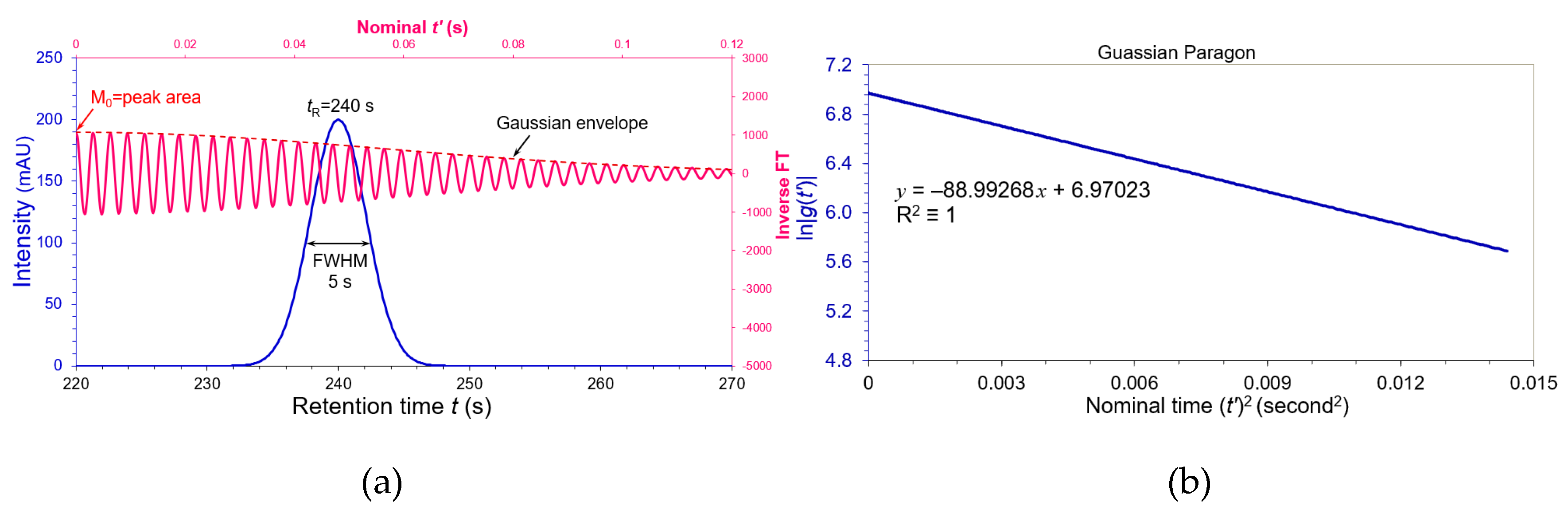
Figure 2.
(a) A pseudo-Voigt peak of 80% Gaussian (blue peak) was simulated with the same chromatographic parameters as those in Figure 1. Its inverse FT sinusoidal wave was depicted in pink versus nominal time t’ (secondary axes), and its envelope dashed brown. (b) A plot of logarithm ln|envelope| versus nominal (t’)2. The trendline (solid brown) of the full 512 data points R2 =0.99535.
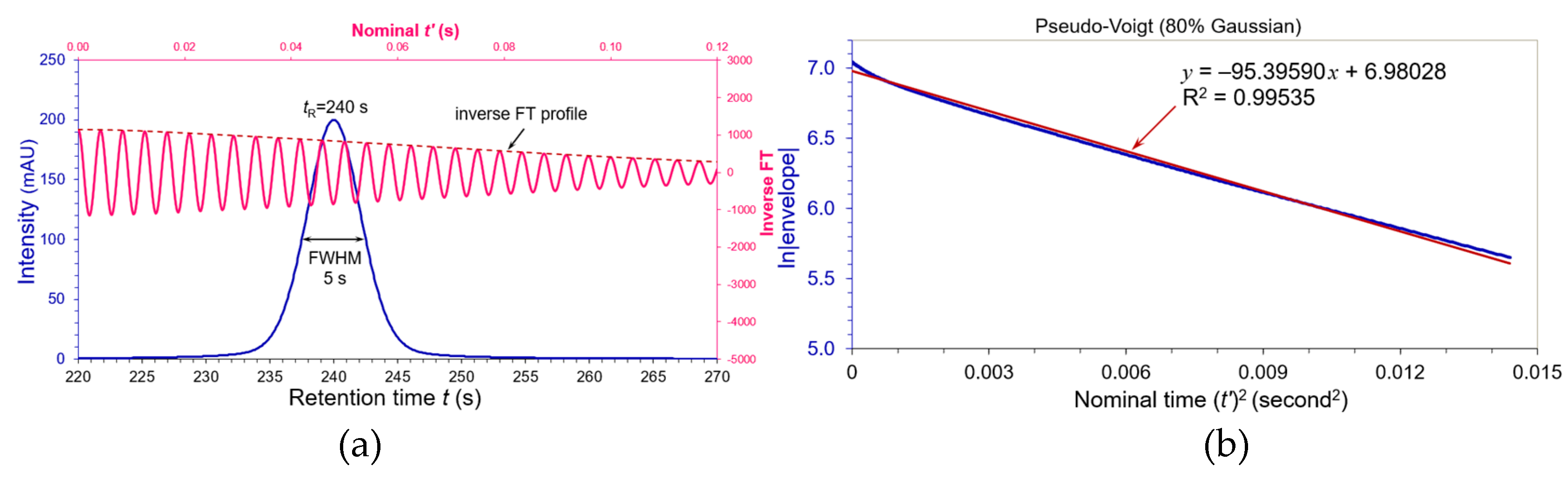
Figure 3.
(a) A pseudo-Voigt peak of 50% Gaussian (blue peak). Its inverse FT sinusoidal wave was depicted in pink versus nominal time t’ (secondary axes), and its envelope dashed brown. The zeroth moment M0 at t’ = 0 (indicated by a red arrow) must be included in the linear regression. (b) A plot of logarithm ln|envelope| versus nominal (t’)2. Its linear regression (solid brown) was performed for the first 94 data points R2 =0.99455.
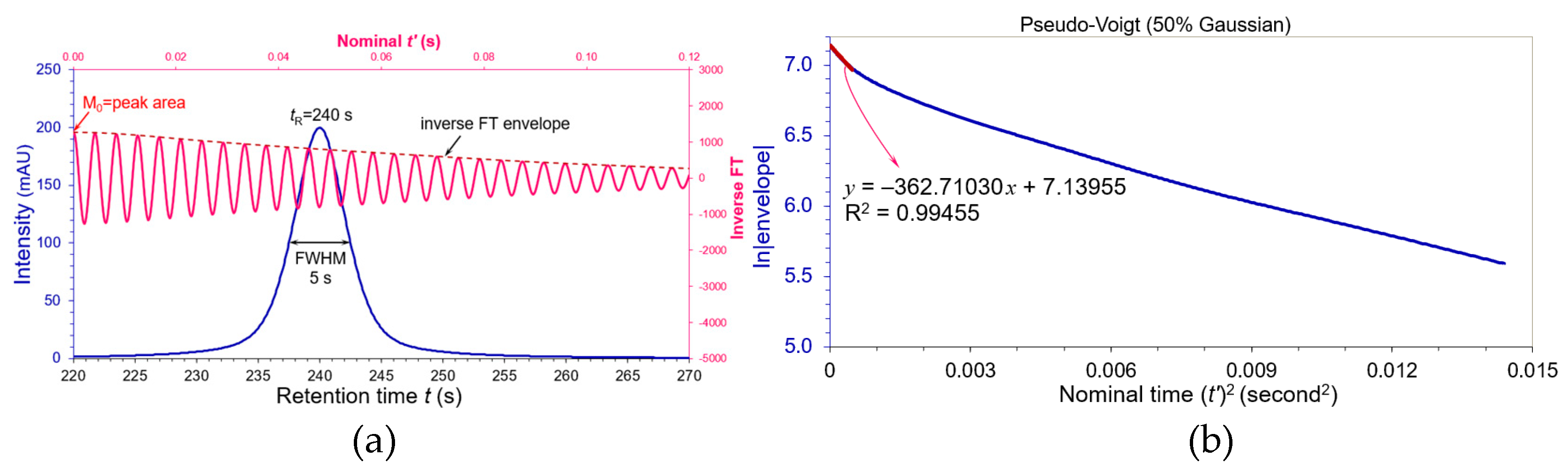
Figure 4.
(a) A fronting PMG peak (blue peak: polynomial τ = –0.144, USP tailing factor AS = 0.800 and apparent FWHM = 5.07291 s) was simulated by the same chromatographic parameters as Figure 1. Its inverse FT sinusoidal wave was depicted in pink versus nominal time t’ (secondary axes), and its envelope dashed brown. (b) A plot of ln|envelope| versus nominal (t’)2. Its trendline (solid brown) of the full 512 data points R2 =0.99832.
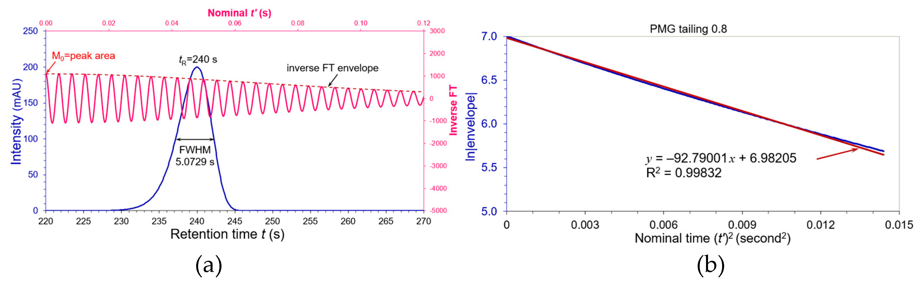
Figure 5.
(a) A tailing PMG peak (blue peak: polynomial τ = +0.1927, USP tailing factor AS = 1.500 and apparent FWHM = 5.13209 s) was simulated by the same chromatographic parameters as Figure 1. Its inverse FT sinusoidal wave was depicted in pink versus nominal time t’ (secondary axes), and its envelope dashed brown. (b) A plot of ln|envelope| versus nominal (t’)2. Its trendline (solid brown) of the full 512 data points R2 =0.99481.
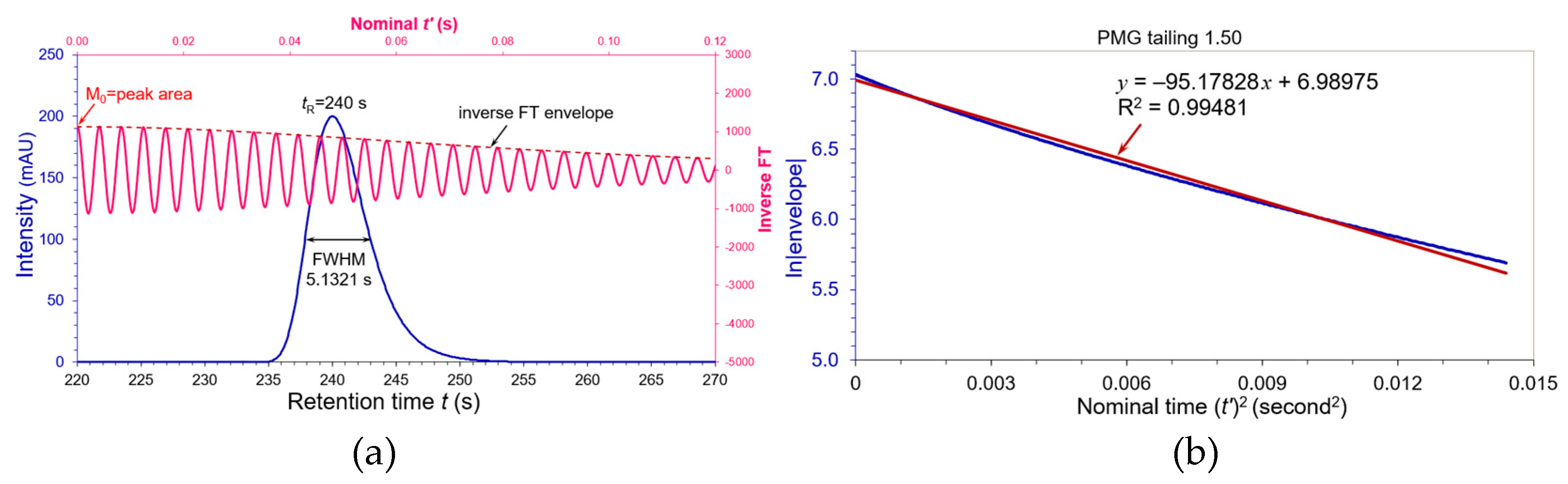
Figure 6.
(a) A tailing PMG peak (blue peak: polynomial τ = +0.2889, USP tailing factor AS = 2.000 and apparent FWHM = 5.30702 s) was simulated by the same chromatographic parameters as Figure 1. Its inverse FT sinusoidal wave was depicted in pink versus nominal time t’ (secondary axes), and its envelope dashed brown. (b) A plot of ln|envelope| versus nominal (t’)2. The trendline (solid brown) of the first 138 data points R2 =0.99459.
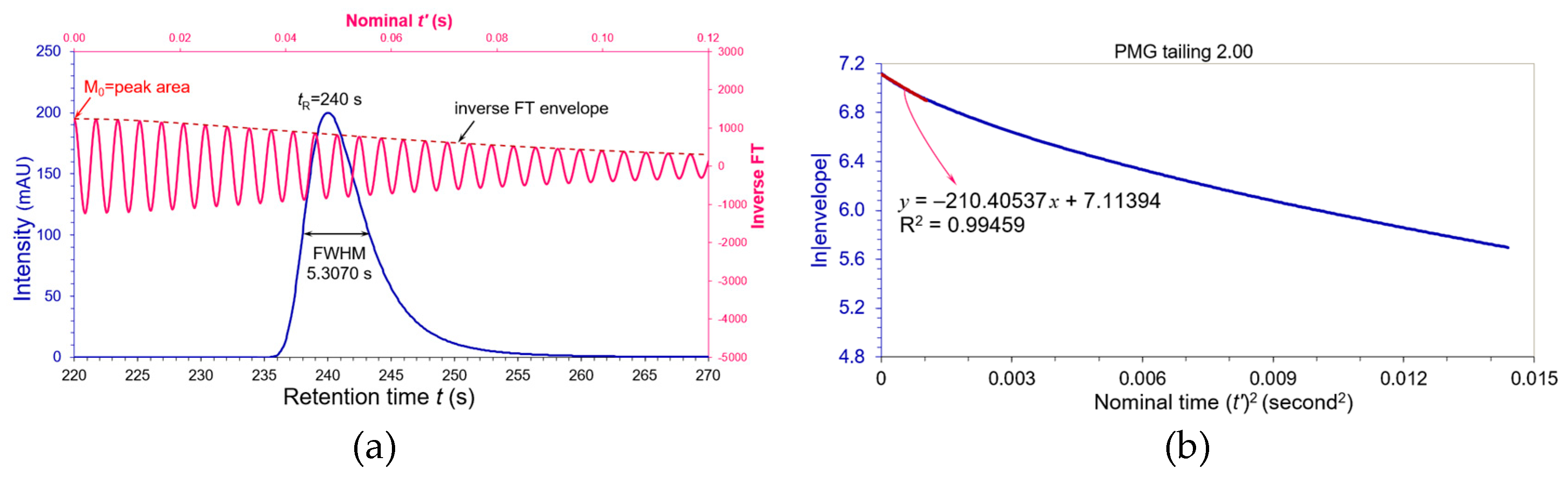
Figure 7.
A histogram of a white Gaussian noise by Python 3.10.14 for the noise testing.

Figure 8.
(a) Intensity of the tailing PMG peak in Figure 5 was reduced to 20 mAU and mixed with a white Gaussian noise at SNR = 10. It retention time and FWHM were both affected. (b) A plot of ln|envelope| of inverse FT versus nominal (t’)2. The trendline (dashed brown) of the full 512 data points with R2 =0.99468.
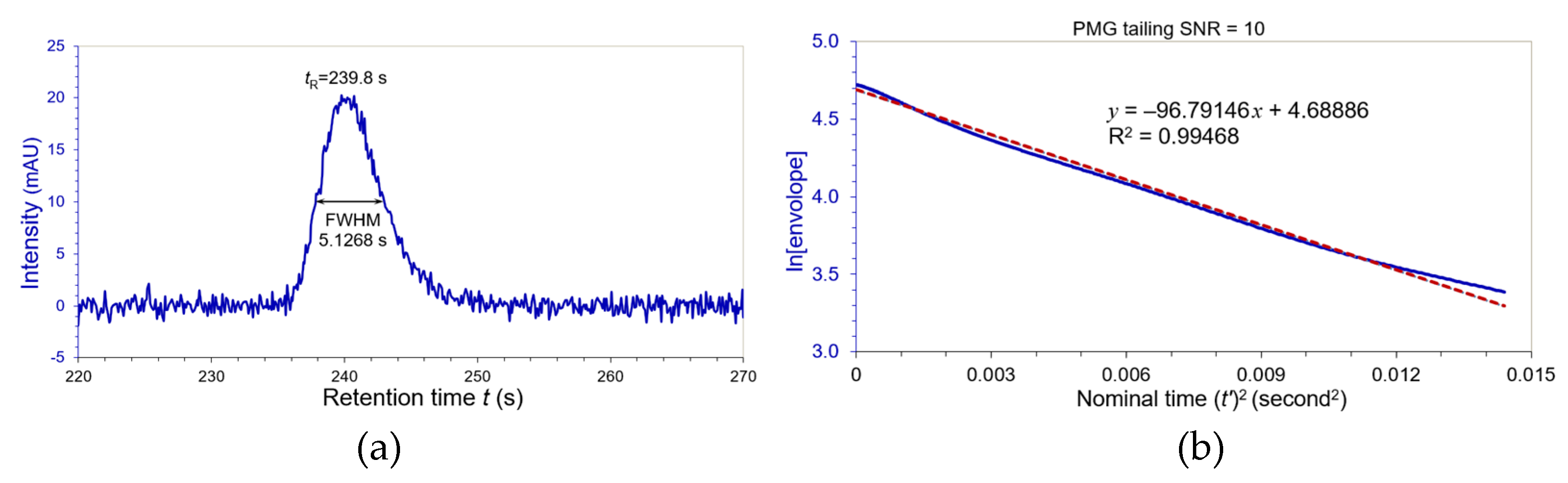
Figure 9.
(a) The Methanol peak (blue peak) acquired from Agilent 6890 II gas chromatograph at retention time 2.8306 minutes with a FWHM 0.0486 minutes. Its tailing factor (= 1.747) was determined as per USP at 5% peak height. The dotted brown peak is its corresponding Gaussian paragon. (b) A linear regression of the inverse FT ln|envelope| versus nominal (t’)2 for the Methanol peak. The linearity of the first 147 data points (solid brown line) R2 =0.99450.
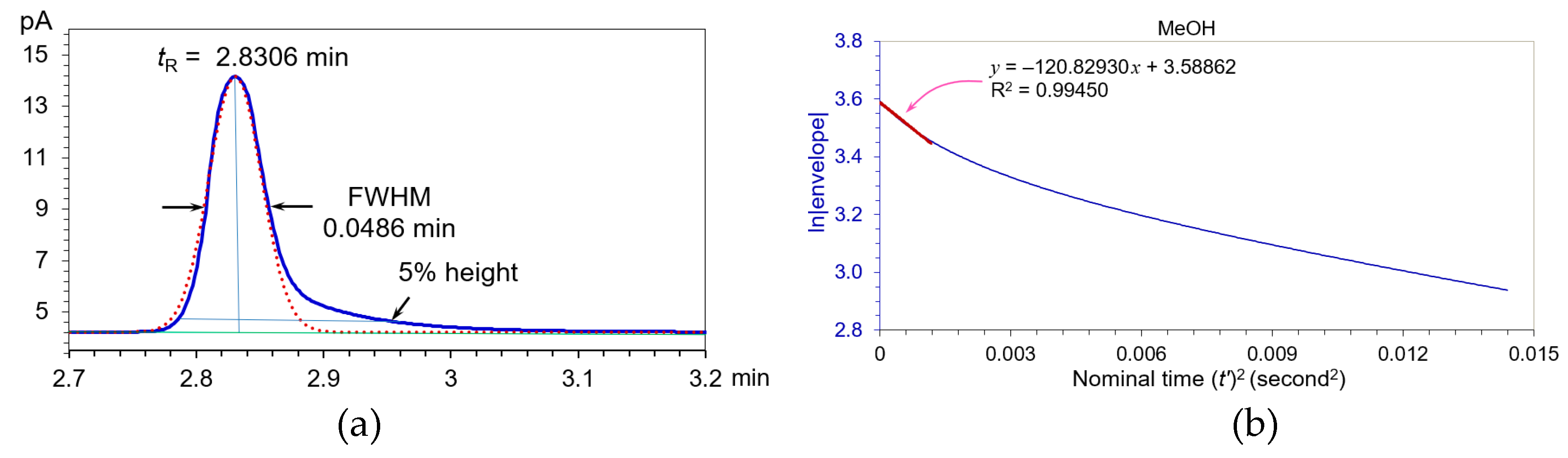
Figure 10.
The n-Hexane peak (blue peak) analyzed simultaneously with the Methanol in Figure 9. Its tR = 6.5106 minutes with a FWHM 0.0715 minutes and tailing factor = 1.008 at 5% peak height. The n-Hexane peak matched well with a corresponding Gaussian paragon (dotted brown peak).
Figure 10.
The n-Hexane peak (blue peak) analyzed simultaneously with the Methanol in Figure 9. Its tR = 6.5106 minutes with a FWHM 0.0715 minutes and tailing factor = 1.008 at 5% peak height. The n-Hexane peak matched well with a corresponding Gaussian paragon (dotted brown peak).


Table 1.
Tailings, FWHMs, equivalent WeG and plate numbers of ten PMG peaks.
| Tailing AS | FWHM (s) | WeG (s) | N (USP) | N (WeG) | N (moment) |
|---|---|---|---|---|---|
| 0.800 | 5.07291 | 5.10556 | 12400 | 12242 | 10357 |
| 0.900 | 5.01433 | 5.02384 | 12691 | 12643 | 12273 |
| 1.125 | 5.01433 | 5.02384 | 12691 | 12643 | 12333 |
| 1.332 | 5.07291 | 5.10556 | 12400 | 12242 | 10477 |
| 1.500 | 5.13209 | 5.17085 | 12116 | 11935 | 8639 |
| 1.533 | 5.14405 | 5.24825 | 12059 | 11585 | 8274 |
| 1.571 | 5.15766 | 5.37839 | 11996 | 11031 | 7864 |
| 1.600 | 5.16822 | 5.47332 | 11947 | 10652 | 7549 |
| 1.750 | 5.22190 | 6.12634 | 11702 | 8502 | 6047 |
| 2.000 | 5.30702 | 7.68814 | 11330 | 5399 | 4178 |
Disclaimer/Publisher’s Note: The statements, opinions and data contained in all publications are solely those of the individual author(s) and contributor(s) and not of MDPI and/or the editor(s). MDPI and/or the editor(s) disclaim responsibility for any injury to people or property resulting from any ideas, methods, instructions or products referred to in the content. |
© 2025 by the authors. Licensee MDPI, Basel, Switzerland. This article is an open access article distributed under the terms and conditions of the Creative Commons Attribution (CC BY) license (http://creativecommons.org/licenses/by/4.0/).
Copyright: This open access article is published under a Creative Commons CC BY 4.0 license, which permit the free download, distribution, and reuse, provided that the author and preprint are cited in any reuse.


