Construction and Evaluation of a Cross-Regional and Cross-Year Monitoring Model for Millet Canopy Phenotype Based on UAV Multispectral Remote Sensing

Accurate, high-throughput canopy phenotyping using UAV-based multispectral remote sensing is critically important for optimizing the management and breeding of foxtail millet in rainfed regions. This study integrated multi-temporal field measurements of leaf water content, SPAD-derived chlorophyll, and leaf area index (LAI) with UAV imagery (red, green, red-edge, near-infrared bands) across two sites and two consecutive years (2023 and 2024) in Shanxi Province, China. Various modeling approaches, including Random Forest, Gradient Boosting, and regularized regressions (e.g., Ridge, Lasso), were evaluated for cross-regional and cross-year extrapolation. Results showed that single-site modeling achieved coefficients of determination (R²) up to 0.95, with mean relative errors of 10%–15% in independent validations. When models were transferred between sites, R² generally remained between 0.50 and 0.70, although SPAD estimates exhibited larger deviations under high-nitrogen conditions. Even under severe drought in 2024, cross-year predictions still attained R² values near 0.60. Among these methods, tree-based models demonstrated strong capability for capturing nonlinear canopy trait dynamics, whereas regularized regressions offered simplicity and interpretability. Incorporating multi-site and multi-year data further enhanced model robustness, increasing R² above 0.80 and markedly reducing average prediction errors. These findings demonstrate that rigorous radiometric calibration and appropriate vegetation index selection enable reliable UAV-based phenotyping for foxtail millet under diverse environments and time frames. The proposed approach thus provides strong technical support for precision management and cultivar selection in semi-arid foxtail millet production systems.

Keywords:

UAV remote sensing

;

Multispectral data

;

Canopy phenotyping

;

Machine learning

;

Foxtail millet

;

Cross-regional extrapolation

;

Cross-year modeling

Subject:

Biology and Life Sciences - Agricultural Science and Agronomy

1. Introduction

Foxtail millet (Setaria italica) plays an essential role in maintaining dietary diversity and nutritional security in China[1-2]. Its exceptional drought tolerance, broad adaptability, high nutritional value, and distinct flavor make it a key cereal in the semi-arid and rainfed regions of northern China [3,4]. Although traditional field methods have extensively explored the physiological traits of foxtail millet (e.g., photosynthetic efficiency, stress resistance, yield formation) [5,6], these approaches often rely on limited datasets (e.g., single-site or single-season trials), falling short of providing comprehensive insights into millet performance across varied environmental conditions, particularly in remote or semi-arid areas with poor soils and scarce rainfall [7,8,9]. Consequently, bridging these knowledge gaps is crucial for improving precision management, pest control, and genetic enhancement of foxtail millet [10,11], yet current methods still lack the capacity for large-scale or multi-year applications.

In northern and northwestern China, the cultivation of foxtail millet spans millions of hectares, underpinning both the livelihoods of numerous smallholders and contributing significantly to modernized agricultural production systems [8,9]. For farmers, the principal concern is maximizing yield, while minimizing inputs such as fertilizer, irrigation, and labor costs. Timely acquisition of critical canopy indicators—including leaf water content, leaf area index (LAI), and leaf nutrient status (e.g., SPAD-derived chlorophyll)—provides direct information on crop growth and final yield potential. Such data also guide precision irrigation and fertilization, thereby boosting resource-use efficiency and lowering overall production expenditure. These benefits hold true for both large-scale operations and smallholder farms, highlighting the broader practical significance of advanced monitoring approaches [12,13].

Recent advances in unmanned aerial vehicle (UAV) remote sensing, notably multispectral platforms spanning blue, green, red-edge, and near-infrared bands, have opened new avenues in high-throughput phenotyping [14,15,16,17]. Compared with traditional methods, UAV-based observations enable more frequent and extensive data collection on crop growth and biochemical attributes, significantly improving spatiotemporal coverage [15,18,19,20,21]. Nevertheless, predictive accuracy often diminishes when models are transferred to new sites or growing seasons, affected by soil variability, climatic fluctuations, and sensor calibration inconsistencies [22,23,24,25]. While data-driven or hybrid models (e.g., PROSAIL, GREENLAB, APSIM) demonstrate potential for cross-environment extrapolation [26,27,28], comprehensive assessments of model robustness in foxtail millet across diverse regions and years remain scarce [29,30]. Although previous research on wheat, rice, and maize has validated UAV multispectral approaches for estimating canopy traits—such as leaf area index, chlorophyll content, and water status [14,15,19,31,32]—transferability to different sites or seasons remains a significant obstacle [33,34,35,36,37]. This challenge becomes even more pronounced for foxtail millet, a relatively understudied crop requiring systematic advancements.

In this study, multi-temporal UAV imagery and ground-based measurements were collected over two consecutive years (2023, a normal precipitation year; and 2024, a severe drought year) from two experimental sites in the Jinzhong region of Shanxi Province, located approximately 50–60 km apart. A comprehensive evaluation of several modeling approaches—including regularized regression, tree-based ensemble methods, and neural networks—was undertaken to maintain high prediction accuracy under cross-regional and cross-year conditions. Specifically, we aim to (1) determine the accuracy of UAV-based multispectral sensing in high-throughput monitoring of key foxtail millet canopy traits (i.e., leaf water content, SPAD-derived chlorophyll, and leaf area index [LAI]); (2) investigate the cross-regional predictive performance of these canopy phenotyping models; (3) assess the cross-year transferability of the resulting spectral prediction models and examine the influence of multi-site data fusion on model robustness; and (4) propose strategies for integrating mechanistic models or advanced data-fusion techniques to further expand model applicability. By constructing a multi-environment modeling framework and conducting systematic validation, this study provides UAV remote sensing–based support for precision management and genetic improvement of foxtail millet in semi-arid and rainfed regions, while also offering a reference for large-scale phenotyping and cross-season adaptation in other minor cereals.

2. Materials and Methods

2.1. Description of the Study Area

Two experimental sites were selected in Shanxi Province, China: the Yuci Lifang Experimental Station (37°51′N, 112°45′E) and the Shanxi Agricultural University Paotuan Experimental Station (37°25′N, 112°36′E), hereafter referred to as LF and PT, respectively. Located in a temperate continental semiarid climate zone, the two sites lie approximately 60 km apart. The soils are classified as cinnamon soils (Calcaric Fluvisols), with an organic matter content of 1.4–1.6%. The region has an annual precipitation of 400–500 mm, an annual mean temperature of 9.5–10.8 °C, an annual sunshine duration of 2,000–3,000 hours, and an annual evaporation of about 1,500–2,300 mm. The experimental fields lie at elevations of 800–900 m above sea level, with a frost-free period of 120–220 days and moderate to relatively high soil fertility. Maize was planted as the previous crop at both stations, creating favorable residual conditions for foxtail millet cultivation.

A single-year field trial (May–October 2023) was conducted at the PT station, covering an area of 3,100 m². Meanwhile, two consecutive years of field trials (May–October 2023 and May–October 2024) were carried out at the LF station, with a trial area of 2,800 m². The two-year dataset from LF provided critical information for cross-year model validation, while the combined trials at both stations supported the construction and evaluation of cross-regional canopy monitoring models.

2.2. Field Experiment Design

The foxtail millet cultivar “Jingu 21” was selected for this study. Planting was carried out with row spacing of 25 cm and plant spacing of 10 cm, in accordance with local standard production practices. Water and fertilizer management, as well as pest and disease control, followed standard agronomic protocols to ensure normal crop growth.

Observations covered key growth stages, including seedling emergence, jointing, heading, grain filling, and maturity. During each growing season in 2023 and 2024, measurements were conducted approximately eight times at regular intervals. For each measurement, six representative quadrats (each 50 cm × 50 cm) were randomly chosen in the field. Within each quadrat, 6–9 millet plants were selected, and their positions were recorded using a high-precision M9 GPS (manufactured by Shanghai Huace Navigation Technology Co., Ltd. , Shanghai, China) to ensure accurate correspondence between the spectral data and actual phenotypic measurements. For each selected plant, measurements were taken of leaf moisture content, SPAD chlorophyll index, and leaf area index (LAI). At the end of the experiment, a total of 200 valid datasets were obtained from PT 2023, LF 2023, and LF 2024, respectively, resulting in a total of 600 valid spectral datasets paired with manually measured phenotypic data of millet plants.

2.3. UAV-Based Multispectral Data Acquisitions

UAV platform (DJI Mavic 3 Multispectral, manufactured by Shenzhen DJI Technology Co., Ltd., Shenzhen, China) equipped with a 4/3-inch visible CMOS sensor and four multispectral CMOS sensors was employed to acquire imagery in four key bands: red (650 nm, 16 nm bandwidth), green (560 nm, 16 nm bandwidth), red-edge (730 nm, 16 nm bandwidth), and near-infrared (860 nm, 26 nm bandwidth). The flight altitude was set at 65 m, with forward and side overlaps of 70% and 80%, respectively, to ensure comprehensive field coverage and high-resolution data acquisition. All flights were conducted between 9:00 AM and 11:00 AM under clear, low-wind conditions to minimize variations in illumination.

Before and after each flight, images of a gray reference board (approximately 0.3 reflectance) and a white reference board (approximately 0.5 reflectance) were captured under similar lighting conditions to determine the reference reflectance for each spectral band. The gain and offset for each band were then calculated based on these calibration images, and pixel-wise radiometric corrections were applied to align the raw images with the reference reflectance. By comparing calibration data collected from multiple flights on the same day and on different dates, consistency was maintained across diverse regions and years.

To further reduce the impact of environmental light fluctuations, cloud interference, and sensor parameter drift, the raw multispectral images underwent radiometric calibration and Z-score normalization. This process yielded calibrated reflectance data that more closely represent the crop’s intrinsic (i.e., “true”) spectral characteristics, thereby improving the accuracy with which subsequent models capture the crop’s physiological status and ensuring a reliable basis for comparison with ground-based measurements.

Finally, the raw multispectral images were processed in DJI Terra (developed by Shenzhen DJI Technology Co., Ltd., Shenzhen, China) to perform image mosaicking, geometric distortion correction, and orthorectification. By incorporating ground control points (GCPs) or using RTK-GPS assistance, the planar positioning error of the orthomosaic was limited to within 1–2 pixels.

2.4. Ground Truthing and Phenotyping

To obtain accurate phenotypic data for millet plants during the growth period and to align these measurements with UAV remote sensing information, the following major canopy parameters were measured in the field:

2): Leaf Area Index (LAI)

LAI was measured using an LAI-2200C canopy analyzer or a comparable scanning method (LAI-2200C manufactured by LI-COR, Inc., Lincoln, Nebraska, USA). Plant density or ground cover was considered to calculate the LAI per unit area, reflecting both the crop’s growth status and photosynthetic potential.

3): Chlorophyll Content (SPAD)

A portable chlorophyll meter (CM 1000 Chlorophyll Meter, Spectrum Technologies, Inc., Aurora, Illinois, USA) was used to measure the top four functional leaves from each selected millet plant. Each measurement was repeated 3–5 times, and the average value was recorded. The SPAD readings indicate the chlorophyll content of the leaves and can be used to assess the plant’s photosynthetic capacity.

4): Canopy Leaf Moisture Content (CLMC)

Simultaneously, the top four functional leaves from each selected millet plant were sampled and immediately sealed in plastic bags. In the laboratory, the fresh weight (Wf) was measured, after which the leaves were placed in an oven at 105 °C for 30 minutes, then dried at 80 °C until a constant weight (Wd) was achieved. Leaf moisture content was calculated using Equation (1):

C L M C = \frac{W_{f -} W_{d}}{W_{f}} \times 100 %

(1)

2.5. Data Preprocessing and Vegetation indices

After radiometric calibration and orthorectification, pixel-level reflectance values were extracted from the four original bands (green, red, red-edge, and near-infrared). Eleven common vegetation indices (Table 1) were then calculated to capture variations in crop chlorophyll content, nitrogen status, and canopy structure.

A total of 15 input variables—including the four multispectral bands plus 11 vegetation indices—were ultimately compiled. Each variable was standardized using the Z-score method to reduce dimensional disparities and improve model stability. Table 1 presents the formulas and references for the 11 vegetation indices employed in this study.

2.6. Model Construction and Evaluation Metrics

In this study, three types of models were selected: linear and regularized regression, tree-based models, and neural networks. Linear and regularized regression included Lasso regression and Ridge regression, both of which have low computational cost and are straightforward to interpret [20,36]. To determine the optimal regularization parameters (e.g., α for Ridge and Lasso), we performed a grid search over a predefined set of values (e.g., 0.01, 0.1, and 1.0) combined with 5-fold cross-validation, selecting the setting that minimized the validation RMSE. The tree-based models included Decision Tree, Random Forest, XGBoost, and LightGBM, which can capture nonlinear features and are easily parallelized [16,31]. For these algorithms, key hyperparameters such as maximum tree depth, number of trees, and learning rate (for boosting models) were tuned via grid search and cross-validation. For instance, we tested max_depth from 4 to 10 (in increments of 2), learning_rate values of {0.01, 0.05, 0.1}, and n_estimators of {100, 300, 500}. We then selected the final configuration based on minimizing RMSE and MRE on the validation set. Neural networks primarily used a Multilayer Perceptron (MLP) architecture. In this study, we adopted two hidden layers, each with 64 neurons, using the ReLU activation function and an Adam optimizer[19,50]. The batch size (32 or 64) and dropout rate (0.2 or 0.5) were chosen by comparing validation errors under multiple runs, ensuring that the model avoided overfitting in smaller datasets.

The coefficient of determination (R²) quantifies how well the model fits observed data, with values approaching 1 indicating stronger explanatory power. Mean Relative Error (MRE) and Maximum Relative Error (MaxRE) represent the average and maximum deviation between predicted and observed values, respectively. The Root Mean Square Error (RMSE) measures how closely predictions conform to actual values (lower RMSE indicates higher predictive accuracy). Additionally, 1:1 Scatter Plots provide a direct comparison between predicted and observed outcomes, while Cumulative Error Distribution Plots illustrate the distribution of errors over a range of values. By leveraging these metrics, we systematically assessed both the accuracy and robustness of the models for canopy traits such as CLMC, SPAD, and LAI across diverse environments and growing seasons, addressing the need for broad spatial and temporal extrapolation.

2.7. Cross-Location and Cross-Year Experimental Scheme

To thoroughly evaluate the model’s spatial extrapolation capability and temporal robustness, the following multi-level experiments and validation strategies were adopted:

1): Single-Location Modeling

Models were independently trained and evaluated using data from Yuci Lifang (2023), Paotuan (2023), and Yuci Lifang (2024), respectively, to assess performance under site-specific conditions.

2): Cross-Location Extrapolation

A model trained on the 2023 data from the Yuci Lifang site was validated on the 2023 data from the Paotuan site (or vice versa), to evaluate the model’s transferability between different geographic locations.

3): Cross-Year Extrapolation

The 2023 data from the Yuci Lifang site were used for training and validated on the 2024 data from the same site, assessing model robustness across different years in the same region. Alternatively, combined data from Yuci 2023 and Paotuan 2023 can be used to train the model and validated on Yuci 2024, allowing for a comparison of predictive improvements gained by data fusion.

4): Multi-Location and Multi-Year Fusion Modeling

Data from multiple sites and different years (e.g., Paotuan 2023 + Yuci 2023 + Yuci 2024) were merged and uniformly radiometrically corrected to build a “universal model.” Independent tests or cross-validation on each subset were then conducted to examine improvements in model generality and stability contributed by data fusion.

3. Results

3.1. Consistency and Calibration Effect of Multispectral Data

Figure 1 depicts the multispectral reflectance characteristics of the millet canopy across four key growth stages, ranging from 30 days after emergence (jointing) to 120 days (maturity). The figure compares three types of spectra: (1) raw data (in red), (2) data corrected against a gray card (≈0.3 reflectance) and a white card (≈0.5 reflectance) (in blue), and (3) data normalized using Z-score standardization (in green). Between 30 and 50 days, the green band (reflectance roughly 0.2–0.5) exhibited pronounced variability due to factors such as ambient light intensity, cloud cover, and UAV altitude, complicating stable representation of crop physiology.

Once calibration was applied, all four bands displayed smoother reflectance curves and a marked reduction in external illumination and atmospheric interference. For example, the green band (Figure 1A) steadily declined from days 30 to 60, consistent with rising chlorophyll levels and canopy coverage, whereas the near-infrared band (Figure 1B) climbed from about 0.8 to 1.5, mirroring rapid canopy expansion. From days 70 to 120, reflectance decreased in all bands, reflecting typical senescence-related spectral patterns and declining water content.

Z-score normalization further constrained the multispectral values to the range of [−2, 2], greatly enhancing cross-stage and cross-site comparability. In the red band (Figure 1C), reflectance declined from days 30 to 60 but rebounded between days 70 and 100, aligning with leaf senescence and chlorophyll degradation. Similarly, the red-edge band (Figure 1D)—highly sensitive to changes in chlorophyll activity and canopy structure—remained relatively stable from days 30 to 60, yet declined sharply from days 70 to 100. This normalization significantly mitigated spatiotemporal variability and highlighted the dynamic spectral changes over the crop’s life cycle.

The smoothed spectral signatures (Figure 1) thus confirm that radiometric calibration and Z-score normalization effectively reduced environmental noise, allowing the inherent canopy-reflectance characteristics of millet to become more apparent. These preprocessed data, therefore, more accurately approximate the “true” reflectance, serving as a robust foundation for subsequent ground validation and model extrapolation.

Overall, the green and red bands exhibited relatively stable fluctuations, driven primarily by chlorophyll absorption and photosynthetic activity, whereas the red-edge and near-infrared bands were more sensitive to changes in canopy structure and biomass—particularly between days 60 and 100. By applying rigorous calibration and normalization, environmental disturbances and UAV parameter fluctuations were substantially minimized, facilitating precise delineation of the millet canopy’s spectral properties at each growth stage. These steps are instrumental in boosting both model accuracy and extrapolation capacity.

3.2. Importance of Spectral Features and Their Effects on Phenotypic Parameters

In this study, we constructed a Random Forest model to predict three canopy traits—leaf water content (Y1), SPAD (Y2), and leaf area index (Y3)—using four multispectral bands (X1–X4) plus 11 derived vegetation indices (X5–X15), forming a total of 15 spectral features. To elucidate the contribution and interaction of these inputs, we employed SHAP (SHapley Additive exPlanations) to interpret the Random Forest predictions. Figure 2 presents SHAP summary plots for Y1 (Figure 2A), Y2 (Figure 2B), and Y3 (Figure 2C). Larger absolute SHAP values denote stronger feature impacts, whereas the SHAP value’s sign (positive or negative) indicates whether the feature exerts a favorable or adverse effect on predictions.

According to Figure 2A, X10 (SAVI) is the most critical feature for leaf water content (Y1). High X10 values (red-colored points) correspond to largely positive SHAP values, implying that increases in SAVI have a generally positive effect on Y1. Following SAVI, X12 (WDRVI) and X9 (RVI) rank next in importance, both showing wide SHAP spreads on the positive and negative ends, indicating notable nonlinear interactions with Y1. Other variables, such as X5 (NDVI) and X13 (TVI), also exhibit moderate to high importance. In contrast, X6 (RDVI) and X14 (DVI) have smaller SHAP ranges, suggesting minimal impact on Y1 and offering possible avenues for feature reduction in practical applications.

For SPAD (Y2), Figure 2B reveals that X10 (SAVI) again ranks highly, but X13 (TVI) and X15 (OSAVI) also stand out, underscoring the relevance of red-edge and near-infrared indices in estimating chlorophyll content. Meanwhile, X2 (NIR) and X6 (RDVI) exhibit bipolar SHAP distributions, implying more complex, nonlinear correlations with SPAD. Conversely, X11 (NDGI) and X14 (DVI) contribute less overall, though they still fine-tune predictive accuracy.

For LAI (Y3), Figure 2C highlights X15 (OSAVI) as having the largest SHAP magnitude, reflecting its strong predictive power. The next most important features, X9 (RVI) and X7 (NLI), also show wide SHAP spreads, illustrating significant nonlinear effects on LAI. While higher RVI or NLI values often yield positive SHAP effects, certain subsets of the data indicate negative influences. X12 (WDRVI) and X5 (NDVI) are likewise influential, whereas X2 (NIR) and X11 (NDGI) remain less significant, contributing only in specific scenarios.

In summary, the 15 spectral features studied demonstrate complex and nonlinear interactions with Y1, Y2, and Y3. X10 (SAVI) is particularly influential for leaf water content and SPAD, while X15 (OSAVI) proves critical for LAI. Other indices (e.g., WDRVI, RVI, NDVI, and TVI) also offer substantial contributions but vary by target trait. These findings suggest that feature selection and modeling approaches should be tailored to specific phenotypic goals. SHAP-based analysis uncovers intricate positive and negative relationships often overlooked by purely linear methods. By combining Random Forest modeling with SHAP interpretability, our approach offers deeper insight into the roles of multispectral and vegetation-index features in foxtail millet canopies. Although individual feature importance varies, the collective use of multiple spectral inputs robustly enhances predictive accuracy for Y1, Y2, and Y3, highlighting promising directions for high-throughput phenotyping and precision agriculture.

3.3. Model Construction and Evaluation under Different Datasets

Using comprehensively radiometrically corrected and normalized UAV data—alongside 11 widely employed vegetation indices—various regression models (linear/regularized), tree-based models (e.g., Random Forest, Gradient Boosting), and a Multilayer Perceptron (MLP) were tested. We categorized these models according to cross-regional, cross-year, and data-fusion strategies to evaluate three key canopy traits in foxtail millet: leaf moisture content (CLMC), SPAD-based chlorophyll content (SPAD), and leaf area index (LAI).

3.3.1. Modeling Results for LF Single-Region Data in 2023

Table 2 presents the evaluation results for the 2023 Yuci Lifang (LF) site. For CLMC, Random Forest (RF) achieved R² = 0.852 (training) and 0.607 (validation), with mean relative errors (MRE) of 3.981% and 7.194%, respectively. This underscores RF’s strong nonlinear capability. Ridge regression ranked second (validation R² = 0.491) but balanced feature constraints and interpretability.

For SPAD, RF again performed the best (R² = 0.946/0.912), with an 11.746% MRE in validation and acceptable maximum relative error (MaxRE). Gradient Boosting (GB) placed second (R² = 0.932/0.902) and showed excellent learning capacity (low training MRE), though its validation RMSE was slightly higher than RF’s.

For LAI, both Ridge and GB excelled. Ridge (R² = 0.758/0.864) had MREs of 11.258%/8.388%, while GB reached a high training R² (0.948) but a lower validation R² (0.806). Both models effectively captured canopy structure. Overall, the LF 2023 dataset demonstrated that RF gave higher accuracy for CLMC and SPAD, while Ridge/GB were competitive for LAI. These results confirm that stringent spectral correction and vegetation index selection enable robust trait estimation.

3.3.2. Modeling Results for Taigu Single-Region Data in 2023

Table 3 presents the modeling outcomes for the 2023 Taigu (PT) dataset. For canopy leaf moisture content (CLMC), Gradient Boosting (GB) achieved the highest R² values (0.944 for training, 0.512 for validation), highlighting its capacity to handle nonlinear interactions, albeit with a moderately lower validation R². Ridge regression produced a similar validation R² (0.482) but yielded a slightly higher MaxRE (31.342%).

In predicting SPAD, GB again led (R² = 0.981/0.866) with an MRE of around 9.810%, effectively capturing chlorophyll dynamics. Lasso regression ranked second but exhibited larger validation errors. These results underscore the strengths of tree-based models in modeling physiological traits such as CLMC and SPAD.

For LAI, the Multilayer Perceptron (MLP) stood out (R² = 0.921/0.785), offering a validation MRE of 14.432% and an acceptable MaxRE of 41.651%. However, MLP models can be prone to overfitting when dataset size is limited or when hyperparameter tuning is inadequate. Overall, results from the 2023 PT site indicate that GB and MLP excel in capturing nonlinear features, while Ridge or Lasso provide better interpretability but prove less robust to extreme samples.

3.3.3. Modeling Results for Yuci Single-Region Data in 2024

Compared to 2023, the 2024 LF dataset (Table 4) showed notably improved accuracy for Gradient Boosting (GB) and Random Forest (RF). For CLMC, both exceeded 0.98 in training R², with validation R² around 0.458–0.513 and low MRE values (e.g., 3.912% for GB). For SPAD, GB again dominated (R² = 0.983/0.956), followed by RF (0.957/0.923). Extended growth-stage sampling likely stabilized model performance.

For LAI, GB reached R² = 0.998 (training) and 0.972 (validation), with a validation MRE of only 4.234%. RF also performed well (R² = 0.989/0.952). Despite severe drought, more comprehensive sampling appears to have mitigated environmental variability. These findings confirm that a combination of multiple vegetation indices and broader sampling supports consistently high accuracy in key canopy traits, even under harsh conditions.

3.3.4. Model Construction and Evaluation under Integrated Dataset

Building on the single-location, single-year analyses, we combined the datasets from PT 2023 (A), LF 2023 (B), and LF 2024 (C) in various ways (A+B, A+C, B+C, and A+B+C). Table 5 summarizes the predictive performance for CLMC, SPAD, and LAI under these fusion scenarios.

Overall, merging datasets generally elevated validation R² values and reduced MRE, particularly in Gradient Boosting (GB) and Random Forest (RF). For example, in A+C, GB reached training/validation R² values of 0.994/0.853, with an MRE of ~3.904%. SPAD predictions often exceeded 0.93 in validation after fusing multi-year or multi-site data, suggesting enhanced adaptability to chlorophyll variability. Although LAI predictions were somewhat more variable, they still demonstrated gains under certain fusion strategies (e.g., A+B with GB). These results underscore that multi-source data fusion consistently bolsters model robustness, highlighting the advantages of diverse environmental inputs for training.

3.4. Cross-Regional and Cross-Year Validation and Evaluation of the Model

3.4.1. Cross-Regional Model Validation and Evaluation in the Same Year

This section explores how models trained at one site perform when applied to another site within the same year. By comparing the top-performing models from the 2023 LF (Longfen) and 2023 PT (Pingtai) datasets, we assessed cross-site transferability via validation on each other’s datasets (Table 6, Figure 3, Figure 4 and Figure 5).

When the 2023 LF-trained model was extrapolated to the 2023 PT dataset, CLMC predictions (Figure 3) achieved R² = 0.502, MRE = 13.55%, and MaxRE = 28.05% (RMSE 0.118). Conversely, models trained on PT 2023 and tested on LF gave an R² of 0.435 but a lower MRE (6.66%), indicating that local environmental factors strongly influence accuracy, yet the overall performance remained acceptable.

For SPAD (Figure 4), the LF-trained model achieved an R² of approximately 0.597 (MRE 14.96%) on PT, whereas the PT-trained model attained R² = 0.831 on LF but exhibited a higher MRE (21.04%). Although outliers were evident, errors tended to cluster in a manageable range, suggesting some practical utility.

For LAI (Figure 5), the LF-based model produced R² = 0.577 (MRE 18.76%) when applied to PT, whereas PT→LF gave R² = 0.584 (MRE 15.57%). The largest discrepancies occurred at high LAI values or under extreme conditions, reflecting moderate environmental influences. Generally, predictions fell within a viable error range.

A comprehensive review of Figure 3, Figure 4 and Figure 5 yields three major insights. Models demonstrate feasible across-site extrapolation for CLMC, SPAD, and LAI within the same year, with most points scattered near the 1:1 line. Soil characteristics, local microclimate, and agronomic management predominantly drive prediction variability, especially under high nitrogen levels or at extreme LAI values. CLMC exhibited more balanced transferability between LF→PT and PT→LF, whereas SPAD and LAI experienced more significant error dispersion, implying that traits linked to local conditions may require additional calibration.

In summary, the 2023 LF-to-PT and PT-to-LF validation confirms that rigorous spectral calibration, normalization, and judicious feature selection enable notable extrapolation capacity. Although soil, climate, and management differences contribute to errors, the models still achieve respectable accuracy for key canopy traits. Future efforts should incorporate broader, multi-region datasets spanning multiple seasons to further improve robustness.

3.4.2. Cross-Year Model Validation and Evaluation for the Following Year

Here, we examine how models trained on the 2023 dataset perform when predicting 2024, evaluating temporal extrapolation. We also investigate whether multi-source data fusion (e.g., combining multi-regional, multi-year samples) enhances 2024 accuracy. Table 7 and Figure 6, Figure 7 and Figure 8 summarize these results.

According to CLMC predictions (Table 7, Figure 6), using only the 2023 LF dataset yielded R² = 0.464 (MRE = 8.06%, MaxRE ≈ 20.69%, RMSE = 0.074) when tested on 2024 LF, implying partial temporal transferability but also biases stemming from weather and management differences. After fusing 2023 LF and 2023 PT data, R² improved to 0.603 (MRE = 5.17%), indicating that multi-regional data help capture leaf moisture variability. Further merging 2023 LF with 2024 LF data raised R² to 0.547 (MRE ≈ 6.19%), suggesting that direct familiarity with the target year benefits predictive stability.

For SPAD (Figure 7), training exclusively on LF 2023 resulted in R² = 0.514 (MRE = 4.21%) on LF 2024, with a MaxRE of 24.72%. Incorporating PT 2023 data elevated R² to 0.658, although extreme values caused higher MaxRE (59.72%). Adding partial 2024 LF data improved R² to 0.971 (MRE ≈ 1.02%), illustrating that prior-year information from the same site can greatly enhance predictive accuracy—though caution is warranted to avoid overlap between training and validation samples.

Regarding LAI (), the baseline 2023 LF→2024 LF model posted R² = 0.583 (MRE = 18.79%), with errors intensifying at high LAI levels. Including PT data raised R² to 0.849 (MRE = 9.80%). Incorporating 2024 LF samples further boosted R² to 0.937, emphasizing once more that multi-environment data mitigate extrapolation risks.

Even though 2023 had normal precipitation and 2024 was marked by severe drought, the models retained satisfactory accuracy across years, demonstrating the significance of spectral calibration, normalization, and feature selection. These findings suggest that augmenting the dataset with additional temporal and environmental heterogeneity would further extend model generalizability.

3.4.3. Model Validation and Evaluation Using Combined Year and Regional Datasets

Building on Sections 3.4.1 and 3.4.2, we next examined how integrating multi-year and multi-regional data influences model construction and extrapolation, validated against the independent 2024 LF dataset. Table 8 and Figure 8 summarize these outcomes.

When data from 2023 and 2024 (including LF and PT) were merged, the model’s CLMC predictions for 2024 LF attained R² = 0.983, MRE ≈ 0.92%, and an RMSE of 0.014 (Figure 9A, 9B), with most errors confined to ±2%, indicating exceptionally high extrapolation accuracy. For SPAD (C, 9D), R² reached 0.947 (MRE = 1.85%, RMSE ≈ 7.32), notably reducing errors relative to single-year or single-region training. LAI predictions (E, 9F) scored an R² of 0.829 (MRE ≈ 20.98%, RMSE = 0.589), although maximum errors remained high (69.06%), implying a need for additional calibration at extremely high LAI values or under extreme conditions.

Collectively, multi-year and multi-region fusion consistently improved model reliability and precision. Two key factors explain these gains: (1) broader source data—encompassing a greater range of climates, management practices, and genetic variations allows the model to “learn” more versatile spectral–phenotypic relationships; and (2) direct coverage of target features—incorporating data from the target site/year aligns training more closely with actual prediction conditions. Nevertheless, LAI under severe drought or unusually dense canopies remains challenging, indicating further adaptation is required.

Overall, the cross-regional and cross-year assessments in Section 3.4 highlight that meticulous radiometric calibration, normalization, and multi-algorithm integration (including linear, regularized, tree-based, and neural network models) yield strong spatial and temporal extrapolation capabilities. Models trained on multi-year, multi-region datasets display notably improved performance for target sites and years, demonstrating robust generalization. Future efforts to gather more extensive temporal series and geographically diverse samples—potentially enriched by high-dimensional environmental and management variables—will further refine these models, providing a solid technical foundation for large-scale, dynamic monitoring and precision management of foxtail millet.

4. Discussion

In this study, UAV-based multispectral data were utilized to monitor key canopy traits in foxtail millet (Setaria italica L.), focusing on their extrapolation capacity across different regions within the same year (2023) and across adjacent years (2023 and 2024). Furthermore, we explored how multi-source data fusion could enhance model robustness. Given that existing UAV-based multispectral research on millet is relatively scarce, our findings, obtained in the semiarid regions of Northern China, provide valuable insights for precision agriculture and phenotyping of minor cereals in larger dryland agricultural zones.

4.1. Cross-Regional Extrapolation within the Same Year

Our cross-validation between two experimental sites (LF and PT) in 2023 revealed that, although local soil texture and climatic factors led to certain prediction deviations, the models maintained generally acceptable extrapolation accuracy for canopy leaf moisture content (CLMC), SPAD, and leaf area index (LAI). Specifically, when applying the model developed from LF data to PT data, CLMC showed moderate prediction deviations, while SPAD displayed a broader error range for some extreme samples (Table 6). This difference may arise from variations in nitrogen application, soil fertility, and local climate, which can strongly influence leaf pigment accumulation and thus SPAD measurements.

Several studies on high-throughput field phenotyping of cereal crops in different regions have reported that environmental heterogeneity (e.g., contrasting precipitation regimes or soil properties) often reduces model accuracy in cross-regional settings [15-17]. Nevertheless, with appropriate radiometric calibration and the inclusion of relevant vegetation indices, models can still achieve workable extrapolation performance for most samples [21]. Our results align with these findings, indicating that UAV-based multispectral approaches have the potential for moderate to high transferability across comparable agronomic settings. However, consistent with other cross-site experiments on wheat and maize [31,32], our research also suggests that additional calibration is needed when regions exhibit extreme differences in temperature, rainfall, or topography.

To further mitigate environmental heterogeneity in cross-regional extrapolation, future work could enlarge the sample size across specific environmental gradients (e.g., soil salinity, slope position) and incorporate site-specific covariates (such as local soil water content or nitrogen levels) either directly into the model or as post-processing correction factors. Moreover, incremental learning or adaptive calibration methods could be introduced so that a small number of local calibration samples in the new region would allow the model to be updated prior to large-scale application [17,22].

4.2. Cross-Year Extrapolation Stability and Influencing Factors

Our cross-year validation at the same site (LF) between 2023 and 2024 demonstrated that predictions remained feasible, even though 2024 experienced severe drought conditions (Section 3.3.2). Model performance generally decreased when only 2023 data were used for extrapolation to 2024; however, the incorporation of multi-source data (e.g., combining 2023 LF with 2023 PT) markedly improved predictive accuracy under extreme environmental scenarios. SPAD exhibited relatively high dispersion in cross-year transfer, suggesting that annual variations in temperature, precipitation, and nutritional status affect leaf pigment accumulation [15,24]. By contrast, CLMC showed slightly more stable response patterns, whereas LAI predictions tended to deviate during late growth under water stress, indicating the model’s need for more extreme drought samples to capture early senescence or reduced canopy expansion accurately.

Comparable cross-year studies on other cereal crops, including maize and wheat, have also reported that climatic anomalies (e.g., extraordinary droughts or excessive rains) can reduce model portability, especially for traits sensitive to environmental stress [16,32,37,28]. The results of our study confirm these challenges in millet, a drought-tolerant crop, thus providing a robust test of the models’ capacity to handle atypical climatic conditions. Despite the notable environmental disparities, the cross-year predictions still achieved acceptable accuracy once stringent radiometric calibration and spectral feature selection were applied.

Future work can enhance cross-year extrapolation by:

Extending multi-year coverage. Long-term datasets (three to five years or more) encompassing normal, wet, and dry seasons would help comprehensively characterize annual variability.

Incorporating dynamic environmental variables. Integrating precipitation, temperature, or soil moisture information into models can help distinguish climatic effects on canopy traits [17,24,47].

Employing time-series or segmentation approaches. Dividing the growth cycle into key developmental stages or using temporal deep-learning architectures (e.g., LSTM, Transformer) could better capture fine-grained phenological responses [25,32].

4.3. Advantages of Multi-Source Data Fusion for Model Transferability

One of the most salient findings of this study was the significant improvement in model extrapolation performance achieved by merging data from multiple regions (LF and PT) and years (2023 and 2024). When trained on multi-source datasets, the models demonstrated not only higher values but also reduced mean and maximum relative errors (Table 5 and Table 8). The underlying mechanism appears to stem from the expanded range of environmental and phenotypic variability encompassed by the fused data, enabling the model to “learn” more generalizable relationships between spectral features and canopy attributes.

Research on other major cereal crops similarly highlights the value of multi-year and multi-regional data integration. For example, multi-sensor and multi-location approaches for wheat and maize phenotyping have significantly improved robustness in trait estimation and yield prediction [15-17,31]. Likewise, efforts in the European Union to integrate wheat phenotypic data from diverse climatic zones reported feasible model transfer across countries [37]. Our work extends these observations to foxtail millet, underlining the necessity of heterogeneous training samples to improve broad-scale and cross-year resilience in model predictions.

Nevertheless, attention should be paid to data quality and consistent protocols when aggregating information from diverse sources [24,37,48]. Key measures include unified radiometric calibration, integration of additional sensor modalities such as hyperspectral or thermal imaging [16,18], and adaptive ensemble modeling—where sub-models trained on each site/year are fused through weighted ensemble or stacking strategies to capture environmental nuances [ 17,31].

4.4. Current Methodological Limitations and Potential Improvements

Despite the promising results, several constraints warrant further investigation.

Limited spatial coverage

The two experimental sites (LF and PT) are only 50–60 km apart, which may not fully capture the diverse ecological conditions of larger millet-growing regions. Future studies should expand to additional provinces or zones (e.g., the Loess Plateau or northwestern arid areas) to validate the true cross-ecozone extrapolation capability [6,24].

Restricted multi-year observations and single extreme climate

Although 2024 provided an extreme drought scenario, only two years of data were collected. Longer-term monitoring (three to five years or beyond) would offer a more comprehensive understanding of interannual variability.

Insufficient variety and genetic diversity

This research focused on the elite foxtail millet variety ‘Jingu 21.’ Other cultivars (e.g., the ‘Zhangzagu’ series) likely exhibit substantial phenotypic differences in leaf color, plant height, and maturity patterns, potentially requiring genotype-specific calibration. Collaboration with breeding programs could enrich the genetic backgrounds included in future models [1-4].

Model interpretability and real-time calibration challenges

Although random forest (RF) and gradient boosting (GB) achieved high accuracy for SPAD and LAI, they offer limited interpretability relative to linear or regularized methods [ 49]. Multilayer perceptron (MLP) can suffer from overfitting in heterogeneous environments [15,50]. Furthermore, the UAV multispectral workflow depends on stable lighting conditions, ground control points, and radiometric calibration boards. Rapid weather changes can still induce measurement uncertainties. Incorporating real-time illumination sensors or automated radiometric calibration modules may further enhance data reliability [17,23].

4.5. Potential for Extension to Other Crops and Climatic Conditions

The workflow established in this study—featuring rigorous calibration, multiple vegetation indices, and data-driven modeling—can be adapted for other cereal and non-cereal crops in both humid and arid regions, provided that training datasets appropriately capture local environmental and phenotypic variability. For example, UAV-based studies on wheat [ 51], sunflower [52], and soybean [53] have shown that robust calibration and multi-temporal sampling can significantly improve the accuracy of canopy trait predictions, even under contrasting climatic conditions. Similarly, ensemble or hybrid modeling approaches have succeeded in quantifying traits like biomass, plant height, and yield components in diverse agroecosystems [54]. These precedents indicate that our methodology could be transferred to other crops or climatic zones, albeit with necessary adjustments—such as incorporating crop-specific phenological parameters or expanding sensor modalities (e.g., thermal or hyperspectral). By systematically adding representative training samples from new environments, the approach can be generalized to increasingly larger regions or more extreme climate scenarios without compromising model precision.

Furthermore, as observed in Section 3.2 of this study, the SHAP-based feature im portance analysis shows that SAVI (X10), WDRVI (X12), RVI (X9), OSAVI (X15), NDVI (X5), and other indices generally rank highly in predicting different canopy traits (CLMC, SPAD, and LAI), but with nuanced differences for each target variable. For instance, SAVI, WDRVI, and RVI stand out for CLMC (Y1), whereas SPAD (Y2) is more strongly influenced by SAVI, TVI (X13), and OSAVI, and LAI (Y3) demonstrates particularly high dependence on OSAVI, RVI, and NLI (X7). This discrepancy in feature importance provides further evidence that the integration of random forest algorithms and multispectral features is capable of capturing the nonlinear and interactive relationships across varying phenotypic traits. It also supports our findings that robust predictive accuracy can be maintained under both cross-regional and cross-year conditions.

Overall, this study shows that combining rigorous UAV-based multispectral imaging, standardized calibration, and multi-source data integration enables feasible and relatively robust predictions of foxtail millet canopy traits over moderate spatial and temporal scales. In comparison with other UAV-based research on major cereals[16,17,21,25], our findings for foxtail millet align with a broader pattern of effective data fusion and advanced machine learning approaches. Modified Content Building on these results, future work can expand to wider geographic areas, incorporate multiple years of data, and leverage richer sensor modalities—potentially enhanced by adaptive learning techniques—to further increase the generality and applicability of these predictive models for foxtail millet breeding and field management. Modified Content

5. Conclusions

This study deployed UAV-based multispectral imaging to monitor three key canopy traits—leaf moisture content (CLMC), SPAD, and leaf area index (LAI)—in foxtail millet (Setaria italica L.) at two experimental sites (LF and PT, approximately 50–60 km apart) across two growing seasons (2023 with normal precipitation and 2024 with severe drought). We thoroughly evaluated the models’ cross-regional and cross-year predictive performance and investigated how multi-source data fusion enhances model robustness. The primary findings are as follows.

Accuracy and feasibility of UAV multispectral monitoring

Under single-site, single-year conditions, rigorous radiometric calibration and a suite of multispectral vegetation indices allowed the models to achieve R² up to approximately 0.95 for CLMC, SPAD, and LAI, with mean relative errors (MRE) around 10%–15%. These results indicate that UAV-based multispectral sensing can effectively capture key physiological and structural traits in foxtail millet canopies. When the models were transferred to a different site in the same year or applied to the subsequent drought year, overall R² values remained around 0.60–0.70, suggesting reasonable portability despite environmental and management contrasts.

Key factors affecting cross-year and cross-regional transferability

Even under severe drought in 2024, the models trained on 2023 data exhibited acceptable performance; incorporating additional data (e.g., from PT) further enhanced accuracy. This underscores the value of diverse training samples in capturing greater environmental variability. Soil differences, nitrogen application levels, and extreme weather conditions (like drought) had stronger impacts on certain traits, notably SPAD, or on high-LAI observations, suggesting that site-specific calibration or additional environmental covariates may be required for these cases.

Advantages of multi-source data fusion and integration with mechanistic models

By combining data from multiple sites and years, the models achieved R^2 values exceeding 0.90 in independent tests, alongside notable reductions in both mean and maximum relative errors. This result highlights the benefit of broader environmental sampling for model generality. Future studies could integrate mechanistic models such as PROSAIL or APSIM and employ advanced data-fusion techniques (e.g., deep learning or temporal modeling) to further improve resilience under extreme environmental conditions and across different growth stages.

Methodological limitations and future directions

The multispectral UAV platform used in this study is well suited to clear, low-wind conditions but may encounter degraded image quality or positioning under complex terrain, strong cloud shadows, or sudden weather changes. Large-scale deployments may necessitate refined flight planning and calibration procedures. Our experiments focused on the widely grown cultivar “Jingu 21” in a typical semi-arid region of Shanxi Province; users planning to apply the models in other millet varieties or more extreme climates should gather supplemental local calibration samples or conduct partial model retraining.

Key spectral predictors (SHAP-based insights)

In addition, SHAP-based feature importance analysis (see Section 3.2) indicated that SAVI (X10), WDRVI (X12), RVI (X9), NDVI (X5), TVI (X13), and OSAVI (X15) serve as pivotal predictors for CLMC (Y1), SPAD (Y2), and LAI (Y3). Their relative rankings and interactions vary among target traits, suggesting that combining raw multispectral bands with derived vegetation indices can more effectively capture the spatiotemporal dynamics of millet canopies and, in turn, enhance model extrapolation and adaptability.

In conclusion, this research provides a validated UAV-based multispectral framework that can reliably estimate foxtail millet canopy traits across moderate spatial scales and at least two consecutive years, offering valuable insights for precision irrigation, fertilization, and cultivar selection in semi-arid agroecosystems. By extending multi-year trials, broadening geographic coverage, and integrating additional sensor types and mechanistic or deep-learning approaches, the modeling framework presented here can be further refined to support large-scale, long-term phenotyping of drought-resilient cereal crops.

Author Contributions

Conceptualization, P.Z. and W.Z; methodology, P.Z. and W.Z.; software, P.Z.; validation, P.Z. and S.J.; formal analysis, P.Z. and W.Z.; investigation, P.Z., Y.Y and W.Z.; resources, P.Z.; data curation, P.Z. and J.Z.; writing—original draft preparation, P.Z. and J.Z.; writing—review and editing, P.Z. and W.Z.; visualization, P.Z. and S.J; supervision, W.Z.; project administration, W.Z.; funding acquisition, P.Z. and W.Z. All authors have read and agreed to the published version of the manuscript.

Funding

The research and the APC was funded by Key Research and Development Project in Shanxi Province (No. 202202140601021); National Key Research and Development Program of China(Grant No. 2021YFD1901101).

Data Availability Statement

The original contributions presented in the study are included in the article, further inquiries can be directed to the corresponding author..

Conflicts of Interest

All authors declare no conflicts of interest.

Abbreviations

The following abbreviations are used in this manuscript:

LR	Linear Regression
RF	Random Forest
GB	Gradient Boosting
MLP	Multilayer perceptron neural networks
LAI	Leaf areas index
CLMC	Canopy Leaf moisture content
X1	Green band reflectance
X2	Red band reflectance
X3	Red-edge band reflectance
X4	Near-infrared band reflectance
X5	NDVI (Normalized Difference Vegetation Index)
X6	RDVI (Renormalized Difference Vegetation Index)
X7	NLI (Non-linear Vegetation Index)
X8	GNDVI (Green Normalized Difference Vegetation Index)
X9	RVI (Ratio Vegetation Index)
X10	SAVI (Soil-Adjusted Vegetation Index)
X11	NDGI (Normalized Difference Greenness Index)
X12	WDRVI (Wide Dynamic Range Vegetation Index)
X13	TVI (Triangular Vegetation Index)
X14	DVI (Difference Vegetation Index)
X15	OSAVI (Optimized Soil-Adjusted Vegetation Index)
Y1	CLMC (Canopy Leaf Moisture Content)
Y2	SPAD (Chlorophyll Content)

References

Nadeem, F.; Ahmad, Z.; Ul Hassan, M.; et al. Adaptation of foxtail millet (Setaria italica L.) to abiotic stresses: a special perspective of responses to nitrogen and phosphate limitations[J]. Frontiers in Plant Science 2020, 11, 187. [Google Scholar] [CrossRef]
Baduni, P.; Maikhuri, R.K.; Bhatt, G.C.; et al. Contribution of millets in food and nutritional security to human being: Current status and future perspectives[J]. Natural Resources Conservation and Research 2024, 7, 5479. [Google Scholar] [CrossRef]
Raut, D.; Sudeepthi, B.; Gawande, K.N.; et al. Millet’s role as a climate resilient staple for future food security: A review[J]. International Journal of Environment and Climate Change 2023, 13, 4542–4552. [Google Scholar]
Singh, R.P.; Qidwai, S.; Singh, O.; et al. Millets for food and nutritional security in the context of climate resilient agriculture: A review[J]. International Journal of Plant & Soil Science 2022, 34, 939–953. [Google Scholar]
Pavithra, K.S.; Senthil, A.; Babu Rajendra Prasad, V.; et al. Variations in photosynthesis associated traits and grain yield of minor millets[J]. Plant Physiology Reports 2020, 25, 418–425. [Google Scholar] [CrossRef]
Reddy, S. Association of photosynthesis of flag leaves with grain yield in pearl millet (Pennisetum glaucum (L. ) R. Br.): Flag leaves association with yield in pearl millet[J]. Annals of Arid Zone 2023, 62, 91–96. [Google Scholar]
Rodríguez, J.P.; Rahman, H.; Thushar, S.; et al. Healthy and resilient cereals and pseudo-cereals for marginal agriculture: Molecular advances for improving nutrient bioavailability[J]. Frontiers in Genetics 2020, 11, 49. [Google Scholar] [CrossRef]
Serba, D.D.; Yadav, R.S.; Varshney, R.K.; et al. Genomic designing of pearl millet: A resilient crop for arid and semi-arid environments[J]. Genomic Designing of Climate-Smart Cereal Crops 2020, 221–286. [Google Scholar]
Tiwari, H.; Naresh, R.K.; Kumar, L.; et al. Millets for food and nutritional security for small and marginal farmers of North West India in the context of climate change: A review[J]. International Journal of Plant & Soil Science 2022, 34, 1694–1705. [Google Scholar]
Jin, S.; Sun, X.; Wu, F.; et al. Lidar sheds new light on plant phenomics for plant breeding and management: Recent advances and future prospects[J]. ISPRS Journal of Photogrammetry and Remote Sensing 2021, 171, 202–223. [Google Scholar] [CrossRef]
Li, D.; Quan, C.; Song, Z.; et al. High-throughput plant phenotyping platform (HT3P) as a novel tool for estimating agronomic traits from the lab to the field[J]. Frontiers in Bioengineering and Biotechnology 2021, 8, 623705. [Google Scholar] [CrossRef] [PubMed]
Wen, T.; Li, J.H.; Wang, Q.; et al. Thermal imaging: The digital eye facilitates high-throughput phenotyping traits of plant growth and stress responses[J]. Science of The Total Environment 2023, 165626. [Google Scholar] [CrossRef] [PubMed]
Reynolds, M.; Chapman, S.; Crespo-Herrera, L.; et al. Breeder friendly phenotyping[J]. Plant Science 2020, 295, 110396. [Google Scholar] [CrossRef] [PubMed]
Yu, T.; Zhou, J.; Fan, J.; et al. Potato leaf area index estimation using multi-sensor unmanned aerial vehicle (UAV) imagery and machine learning[J]. Remote Sensing 2023, 15, 4108. [Google Scholar] [CrossRef]
Cao, X.; Liu, Y.; Yu, R.; et al. A comparison of UAV RGB and multispectral imaging in phenotyping for stay green of wheat population[J]. Remote Sensing 2021, 13, 5173. [Google Scholar] [CrossRef]
Shu, M.; Fei, S.; Zhang, B.; et al. Application of UAV multisensor data and ensemble approach for high-throughput estimation of maize phenotyping traits[J]. Plant Phenomics 2022. [Google Scholar] [CrossRef]
Fei, S.; Hassan, M.A.; Xiao, Y.; et al. UAV-based multi-sensor data fusion and machine learning algorithm for yield prediction in wheat[J]. Precision Agriculture 2023, 24, 187–212. [Google Scholar] [CrossRef]
Guo, Q.; Su, Y.; Hu, T.; et al. Lidar boosts 3D ecological observations and modelings: A review and perspective[J]. IEEE Geoscience and Remote Sensing Magazine 2020, 9, 232–257. [Google Scholar] [CrossRef]
Li, Z.; Chen, Z.; Cheng, Q.; et al. UAV-based hyperspectral and ensemble machine learning for predicting yield in winter wheat[J]. Agronomy 2022, 12, 202. [Google Scholar] [CrossRef]
Osco, L.P.; Junior, J.M.; Ramos, A.P.M.; et al. Leaf nitrogen concentration and plant height prediction for maize using UAV-based multispectral imagery and machine learning techniques[J]. Remote Sensing 2020, 12, 3237. [Google Scholar] [CrossRef]
Fan, J.; Zhou, J.; Wang, B.; et al. Estimation of maize yield and flowering time using multi-temporal UAV-based hyperspectral data[J]. Remote Sensing 2022, 14, 3052. [Google Scholar] [CrossRef]
Hamrouni, Y.; Paillassa, E.; Chéret, V.; et al. From local to global: A transfer learning-based approach for mapping poplar plantations at national scale using Sentinel-2[J]. ISPRS Journal of Photogrammetry and Remote Sensing 2021, 171, 76–100. [Google Scholar] [CrossRef]
Nex, F.; Armenakis, C.; Cramer, M.; et al. UAV in the advent of the twenties: Where we stand and what is next[J]. ISPRS Journal of Photogrammetry and Remote Sensing 2022, 184, 215–242. [Google Scholar] [CrossRef]
Inoue, Y. Satellite-and drone-based remote sensing of crops and soils for smart farming–a review[J]. Soil Science and Plant Nutrition 2020, 66, 798–810. [Google Scholar] [CrossRef]
Azzari, G.; Jain, M.; Lobell, D.B. Towards fine resolution global maps of crop yields: Testing multiple methods and satellites in three countries[J]. Remote Sensing of Environment 2017, 202, 129–141. [Google Scholar] [CrossRef]
Singh, P.; Srivastava, P.K.; Verrelst, J.; et al. High resolution retrieval of leaf chlorophyll content over Himalayan pine forest using Visible/IR sensors mounted on UAV and radiative transfer model[J]. Ecological Informatics 2023, 75, 102099. [Google Scholar] [CrossRef]
Cheng, J.; Han, S.; Verrelst, J.; et al. Deciphering maize vertical leaf area profiles by fusing spectral imagery data and a bell-shaped function[J]. International Journal of Applied Earth Observation and Geoinformation 2023, 120, 103355. [Google Scholar] [CrossRef]
Cheng, Z.; Meng, J.; Shang, J.; et al. Generating time-series LAI estimates of maize using combined methods based on multispectral UAV observations and WOFOST model[J]. Sensors 2020, 20, 6006. [Google Scholar] [CrossRef]
Wang, Y.; Feng, L.; Zhang, Z.; et al. An unsupervised domain adaptation deep learning method for spatial and temporal transferable crop type mapping using Sentinel-2 imagery[J]. ISPRS Journal of Photogrammetry and Remote Sensing 2023, 199, 102–117. [Google Scholar] [CrossRef]
Xu, Y.; Ma, Y.; Zhang, Z. Self-supervised pre-training for large-scale crop mapping using Sentinel-2 time series[J]. ISPRS Journal of Photogrammetry and Remote Sensing 2024, 207, 312–325. [Google Scholar] [CrossRef]
Cheng, Q.; Ding, F.; Xu, H.; et al. Quantifying corn LAI using machine learning and UAV multispectral imaging[J]. Precision Agriculture 2024, 1–23. [Google Scholar] [CrossRef]
Yang, G.; Li, Y.; Yuan, S.; et al. Enhancing direct-seeded rice yield prediction using UAV-derived features acquired during the reproductive phase[J]. Precision Agriculture 2024, 25, 1014–1037. [Google Scholar] [CrossRef]
Karthikeyan, L.; Chawla, I.; Mishra, A.K. A review of remote sensing applications in agriculture for food security: Crop growth and yield, irrigation, and crop losses[J]. Journal of Hydrology 2020, 586, 124905. [Google Scholar] [CrossRef]
Gibson, P.B.; Chapman, W.E.; Altinok, A.; et al. Training machine learning models on climate model output yields skillful interpretable seasonal precipitation forecasts[J]. Communications Earth & Environment 2021, 2, 159. [Google Scholar]
Kang, Y.; Ozdogan, M.; Zhu, X.; et al. Comparative assessment of environmental variables and machine learning algorithms for maize yield prediction in the US Midwest[J]. Environmental Research Letters 2020, 15, 064005. [Google Scholar] [CrossRef]
Feng, P.; Wang, B.; Li Liu, D.; et al. Dynamic wheat yield forecasts are improved by a hybrid approach using a biophysical model and machine learning technique[J]. Agricultural and Forest Meteorology 2020, 285, 107922. [Google Scholar] [CrossRef]
Weiss, M.; Jacob, F.; Duveiller, G. Remote sensing for agricultural applications: A meta-review[J]. Remote Sensing of Environment 2020, 236, 111402. [Google Scholar] [CrossRef]
Huang, S.; Tang, L.; Hupy, J.P.; et al. A commentary review on the use of normalized difference vegetation index (NDVI) in the era of popular remote sensing[J]. Journal of Forestry Research 2021, 32, 1–6. [Google Scholar] [CrossRef]
Chen, J.M. Evaluation of vegetation indices and a modified simple ratio for boreal applications[J]. Canadian Journal of Remote Sensing 1996, 22, 229–242. [Google Scholar] [CrossRef]
Liu, Y.; Sun, Q.; Huang, J.; et al. Estimation of potato above ground biomass based on UAV multispectral images[J]. Spectroscopy and Spectral Analysis 2021, 41, 2549–2555. [Google Scholar]
Gitelson, A.A.; Kaufman, Y.J.; Merzlyak, M.N. Use of a green channel in remote sensing of global vegetation from EOS-MODIS[J]. Remote Sensing of Environment 1996, 58, 289–298. [Google Scholar] [CrossRef]
Pearson, R.L.; Miller, L.D. Remote mapping of standing crop biomass for estimation of the productivity of the shortgrass prairie[J]. Remote Sensing of Environment 1972, VIII, 1355. [Google Scholar]
Huete, A. A soil-adjusted vegetation index (SAVI)[J]. Remote Sensing of Environment 1988, 25, 295–309. [Google Scholar] [CrossRef]
Khan, N.M.; Rastoskuev, V.V.; Sato, Y.; et al. Assessment of hydrosaline land degradation by using a simple approach of remote sensing indicators[J]. Agricultural Water Management 2005, 77, 96–109. [Google Scholar] [CrossRef]
Gitelson, A.A. Wide dynamic range vegetation index for remote quantification of biophysical characteristics of vegetation[J]. Journal of Plant Physiology 2004, 161, 165–173. [Google Scholar] [CrossRef]
Zhang, S.; Zhao, G.; Lang, K.; et al. Integrated Satellite, Unmanned Aerial Vehicle (UAV) and Ground Inversion of the SPAD of Winter Wheat in the Reviving Stage[J]. Sensors 2019, 19, 1485. [Google Scholar] [CrossRef]
Wu, B.; Zhang, M.; Zeng, H.; et al. Challenges and opportunities in remote sensing-based crop monitoring: A review[J]. National Science Review 2023, 10, nwac290. [Google Scholar] [CrossRef]
Jin, X.; Zarco-Tejada, P.J.; Schmidhalter, U.; et al. High-throughput estimation of crop traits: A review of ground and aerial phenotyping platforms[J]. IEEE Geoscience and Remote Sensing Magazine 2020, 9, 200–231. [Google Scholar] [CrossRef]
Zhang, Y.; Zhang, R.; Ma, Q.; et al. A feature selection and multi-model fusion-based approach of predicting air quality[J]. ISA Transactions 2020, 100, 210–220. [Google Scholar] [CrossRef]
Alqadhi, S.; Mallick, J.; Balha, A.; et al. Spatial and decadal prediction of land use/land cover using multi-layer perceptron-neural network (MLP-NN) algorithm for a semi-arid region of Asir, Saudi Arabia[J]. Earth Science Informatics 2021, 14, 1547–1562. [Google Scholar] [CrossRef]
Fang, Y.; Qiu, X.; Guo, T.; Wang, Y.; Cheng, T.; Zhu, Y.; et al. An automatic method for counting wheat tiller number in the field with terrestrial LiDAR[J]. Plant Methods 2020, 16, 1–14. [Google Scholar] [CrossRef] [PubMed]
Centorame, L.; Gasperini, T.; Ilari, A.; Del Gatto, A.; Foppa Pedretti, E. An overview of machine learning applications on plant phenotyping, with a focus on sunflower[J]. Agronomy 2024, 14, 719. [Google Scholar] [CrossRef]
Zhou, J.; Zhou, J.; Ye, H.; Ali, M.L.; Chen, P.; Nguyen, H.T. Yield estimation of soybean breeding lines under drought stress using unmanned aerial vehicle-based imagery and convolutional neural network[J]. Biosystems Engineering 2021, 204, 90–103. [Google Scholar] [CrossRef]
Pantazi, X.E.; Moshou, D.; Alexandridis, T.; Whetton, R.L.; Mouazen, A.M. Wheat yield prediction using machine learning and advanced sensing techniques[J]. Computers and Electronics in Agriculture 2016, 121, 57–65. [Google Scholar] [CrossRef]

Figure 1. Radiometric correction using gray and white cards, along with Z-score standardization, was applied to the DN brightness values of the multispectral data in four bands selected across different times and locations. Panel A represents the Green band spectrum, Panel B represents the NIR band spectrum, Panel C represents the RED band spectrum, and Panel D represents the RedEdge band spectrum after radiometric correction and normalization.

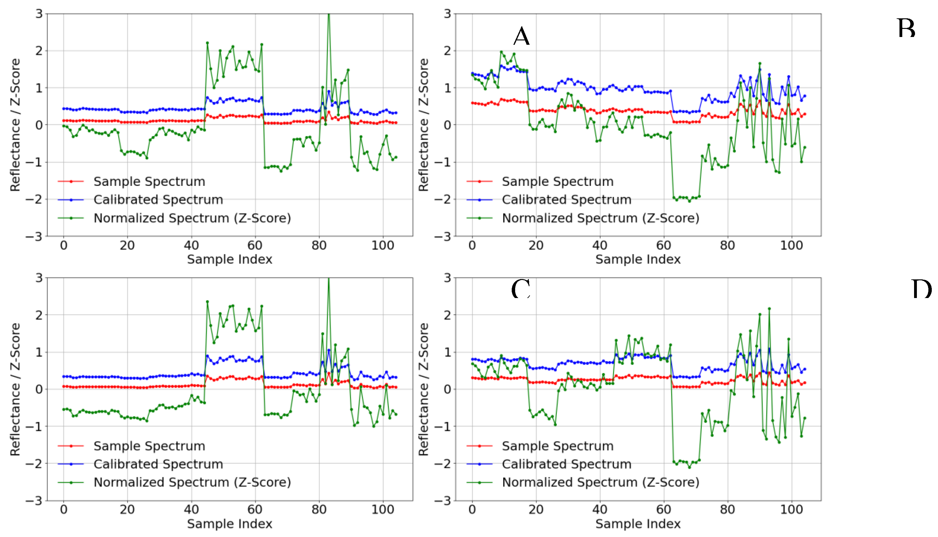
Figure 2. SHAP analysis results of spectral features (X1–X4) and vegetation indices (X5–X15) for different foxtail millet canopy traits(Y1–Y4). Panel (A) presents the SHAP summary plot for predicting canopy trait Y1 using X1–X15 as input variables. Panel (B) displays the SHAP summary plot for predicting Y2 based on X1–X15.Panel (C) illustrates the SHAP summary plot for predicting Y3 using X1–X15 as input variables.

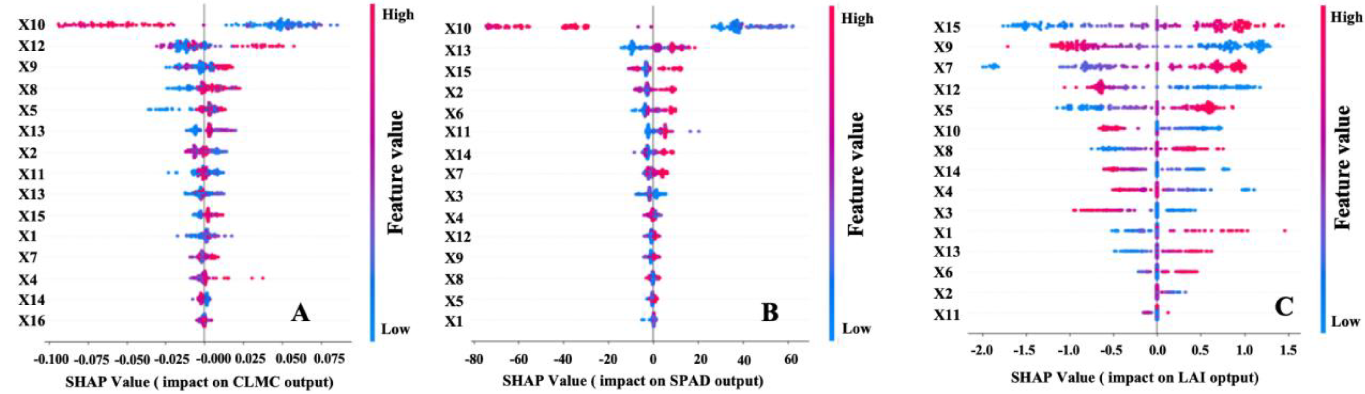
Figure 3. Cross-regional validation results of canopy leaf moisture content (CLMC) models for foxtail millet. A: Validation of the optimal model constructed using the 2023 LF dataset on the 2023 PT dataset, B: Cumulative probability distribution of relative errors for Panel A, C: Validation of the optimal model constructed using the 2023 PT dataset on the 2023 LF dataset, D: Cumulative probability distribution of relative errors for Panel C

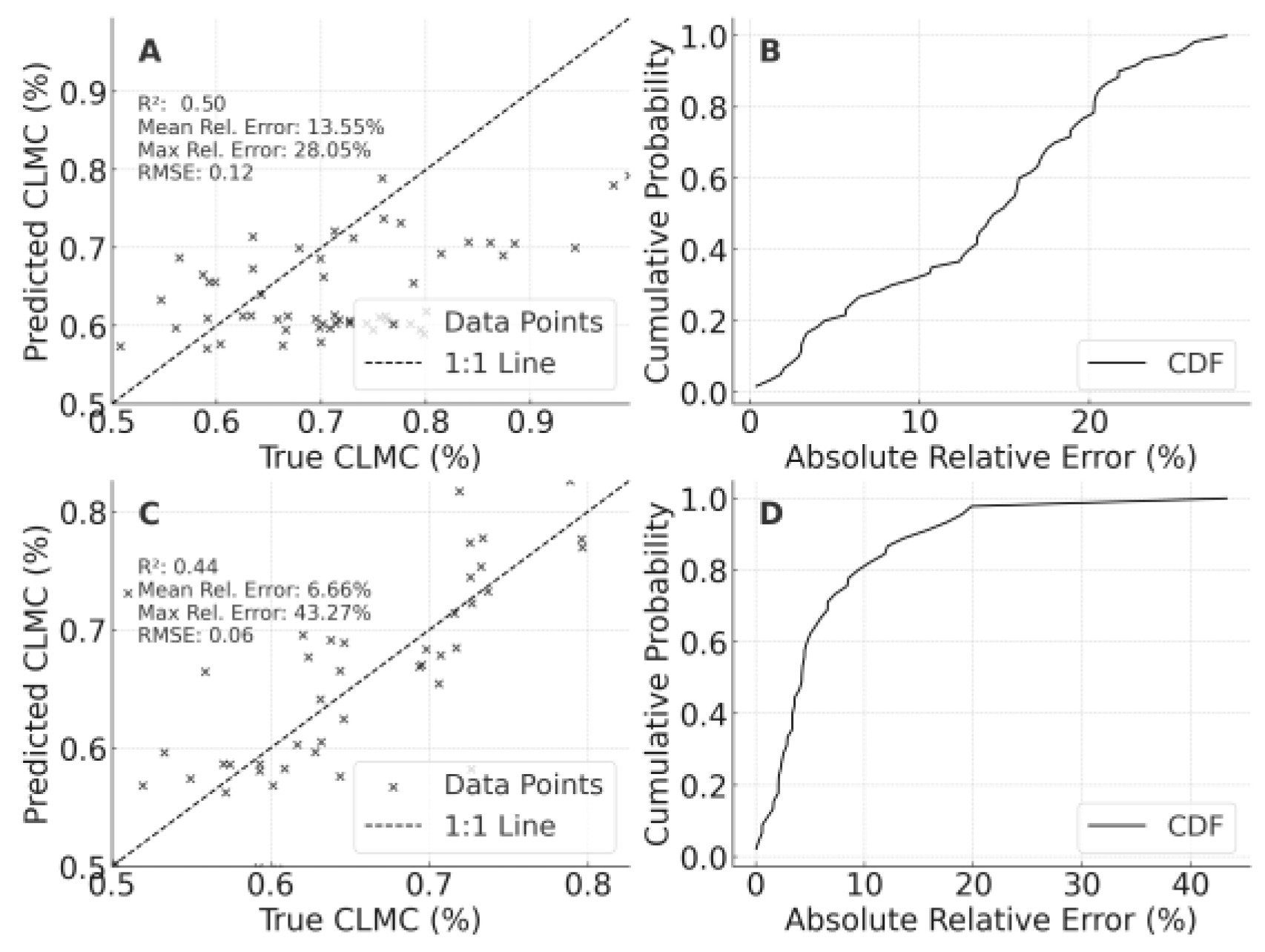
Figure 4. Cross-regional validation results of SPAD models for foxtail millet. A: Validation of the optimal model constructed using the 2023 LF dataset on the 2023 PT dataset; B: Cumulative probability distribution of relative errors for Panel A; C: Validation of the optimal model constructed using the 2023 PT dataset on the 2023 LF dataset,; D: Cumulative probability distribution of relative errors for Panel C.

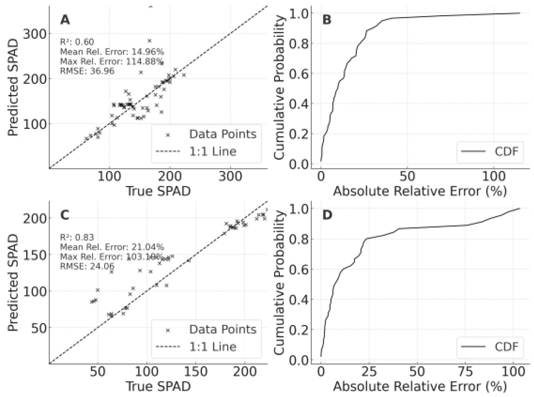
Figure 5. Cross-regional validation results of leaf area index (LAI) models for foxtail millet. A: Validation of the optimal model constructed using the 2023 LF dataset on the 2023 PT dataset; B: Cumulative probability distribution of relative errors for Panel A; C: Validation of the optimal model constructed using the 2023 PT dataset on the 2023 LF dataset,; D: Cumulative probability distribution of relative errors for Panel C.

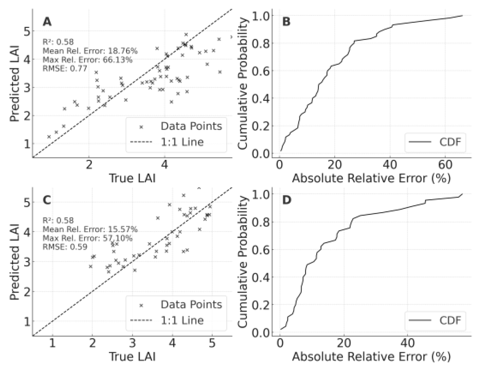
Figure 6. Cross-year validation results of canopy leaf moisture content (CLMC) models for foxtail millet. A: Validation of the optimal model constructed using the 2023 LF dataset on the 2024 LF dataset, B: Cumulative probability distribution of relative errors for Panel A, C: Validation of the optimal model constructed using the integrated 2023 PT and 2023 LF datasets on the 2024 LF dataset,D: Cumulative probability distribution of relative errors for Panel C,E: Validation of the optimal model constructed using the integrated 2023 LF and 2024 LF datasets on the 2024 LF dataset,F: Cumulative probability distribution of relative errors for Panel E.

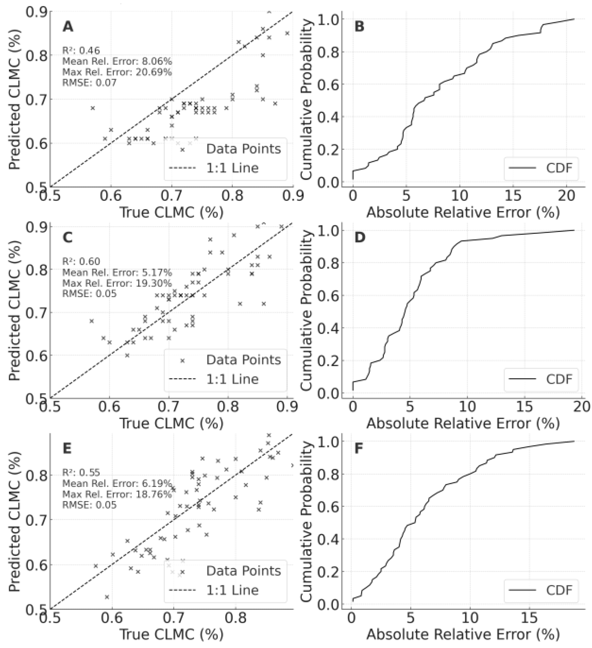
Figure 7. Cross-year validation results of SPAD models for foxtail millet. A: Validation of the optimal model constructed using the 2023 LF dataset on the 2024 LF dataset,B: Cumulative probability distribution of relative errors for Panel A,C: Validation of the optimal model constructed using the integrated 2023 PT and 2023 LF datasets on the 2024 LF dataset,D: Cumulative probability distribution of relative errors for Panel C,E: Validation of the optimal model constructed using the integrated 2023 LF and 2024 LF datasets on the 2024 LF dataset,F: Cumulative probability distribution of relative errors for Panel E.

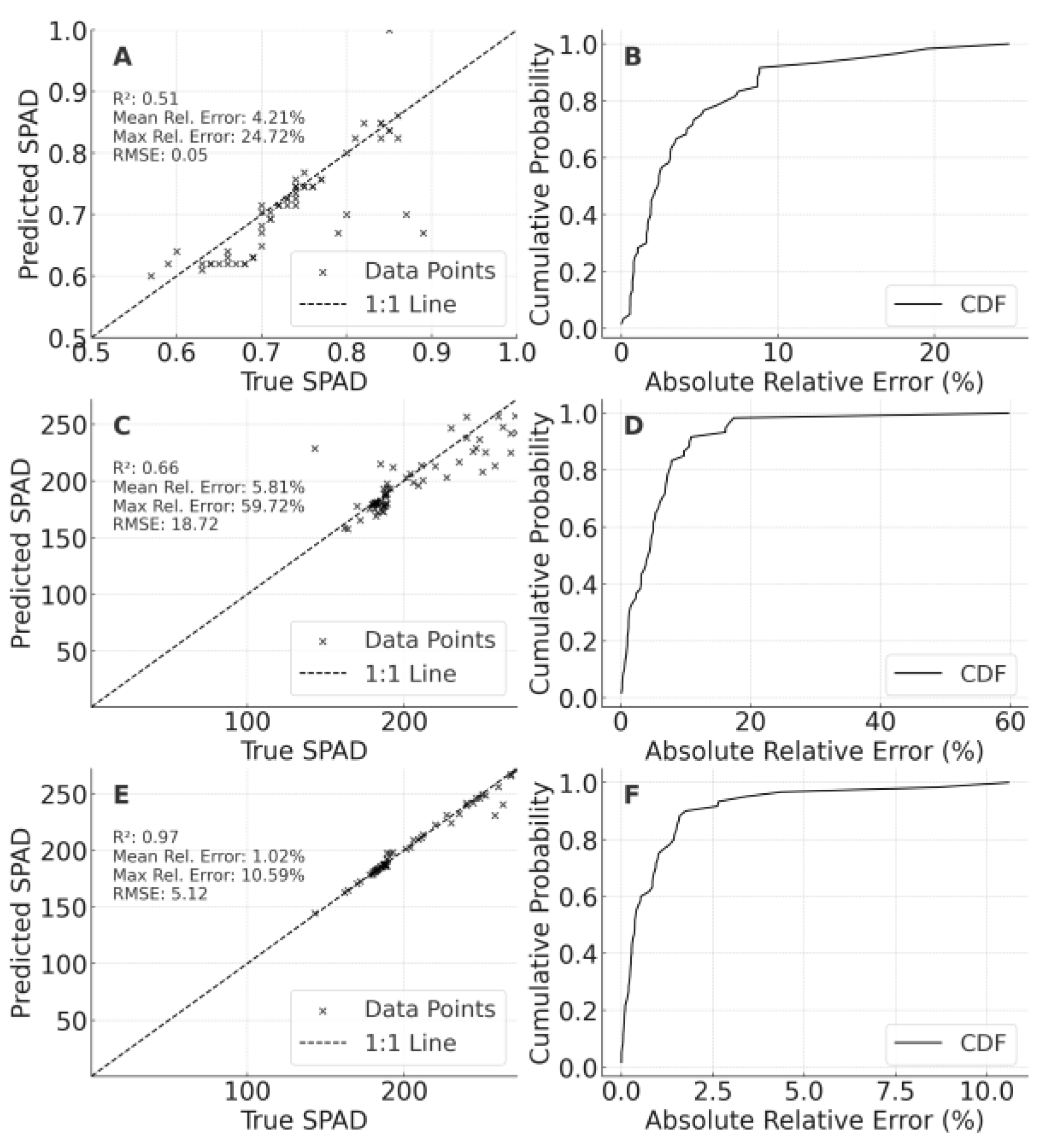
Figure 8. Cross-year validation results of leaf area index (LAI) models for foxtail millet. Panel A: Validation of the optimal model constructed using the 2023 LF dataset on the 2024 LF dataset. Panel B: Cumulative probability distribution of relative errors for scenario A; Panel C: Validation of the optimal model constructed using the integrated 2023 PT and 2023 LF datasets on the 2024 LF dataset; Panel D: Cumulative probability distribution of relative errors for scenario C.; Panel E: Validation of the optimal model constructed using the integrated 2023 LF and 2024 LF datasets on the 2024 LF dataset.; Panel F: Cumulative probability distribution of relative errors for scenario E.

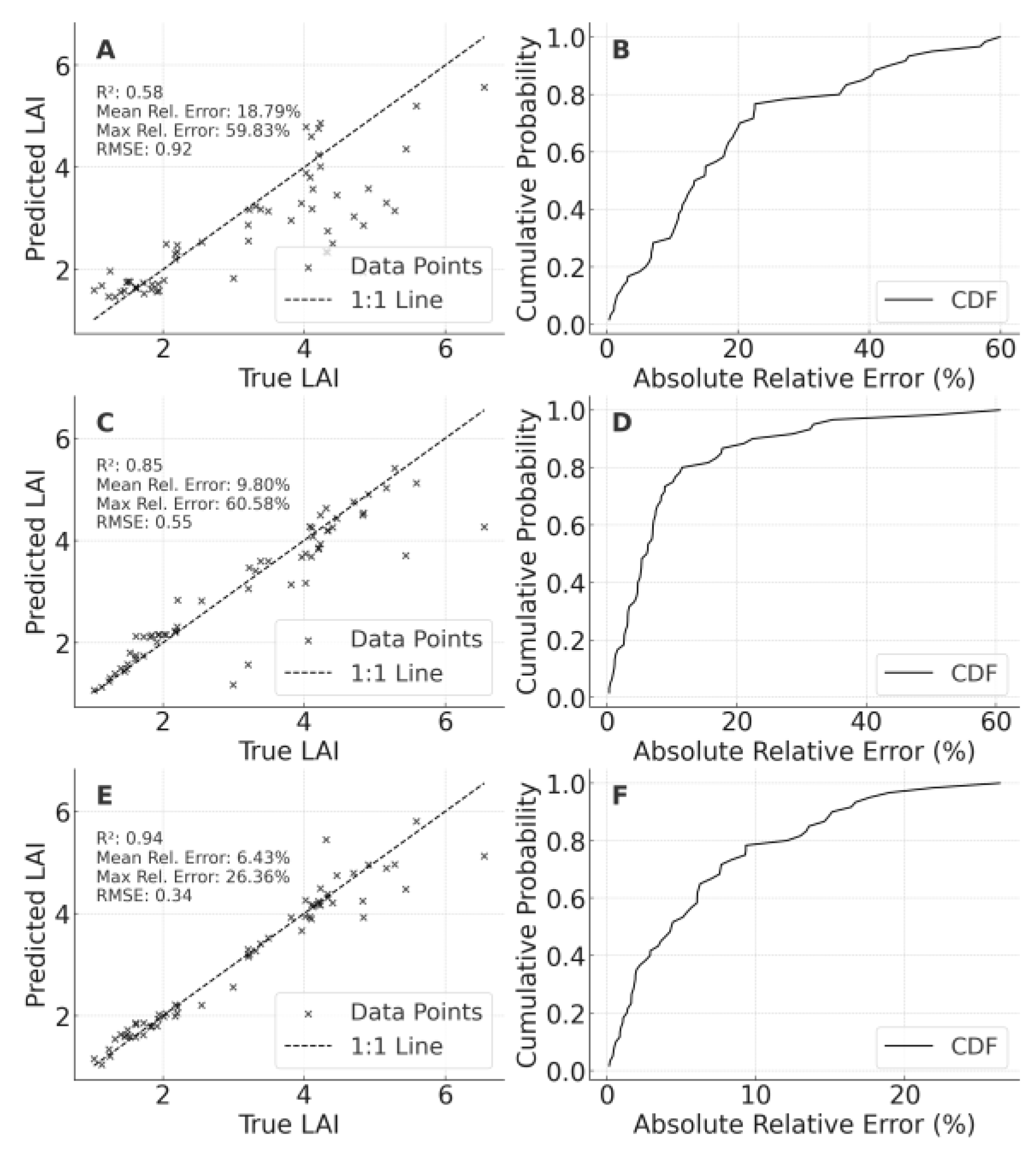
Figure 9. Validation and evaluation results of models constructed using integrated temporal and spatial datasets. Panel A: Cross-validation of canopy leaf moisture content predictions. Panel B: Cumulative probability distribution of relative errors for Panel A. Panel C: Cross-validation of SPAD predictions. Panel D: Cumulative probability distribution of relative errors for Panel C. Panel E: Cross-validation of leaf area index predictions. Panel F: Cumulative probability distribution of relative errors for Panel E.

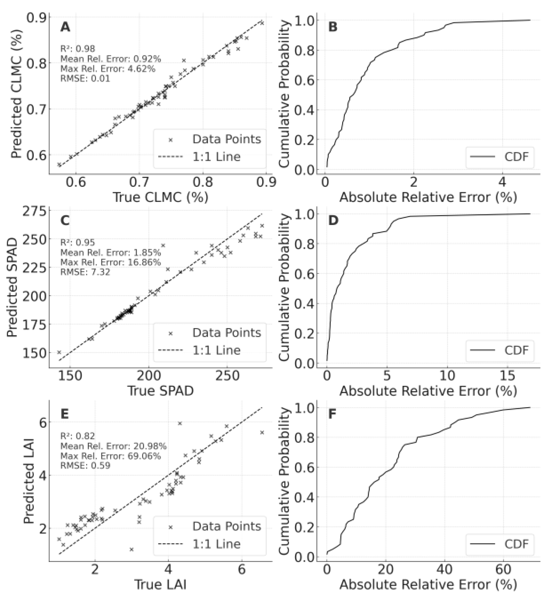
Table 1. The 11 indices and their calculation methods used in the paper.

Index Number	Vegetation Index	Calculation Formula	Reference
1	Normalized Difference Vegetation Index (NDVI)	$(N i r - R) / (N i r + R)$	[38]
2	Renormalized Difference Vegetation Index (RDVI)	$(N i r - R) / (\sqrt{N i r + R})$	[39]
3	Nonlinear Vegetation Index (NLI)	$({N i r}^{2} - R) / (({N i r}^{2} + R))$	[40]
4	Green Normalized Difference Vegetation Index (GNDVI)	$(N i r - G) / (N i r + G)$	[41]
5	Ratio Vegetation Index (RVI)	$(N i r) / (R)$	[42]
6	Soil-Adjusted Vegetation Index (SAVI)	$1.5 \cdot (N i r - R) / (N i r + R + 0.5)$	[43]
7	Normalized Difference Green Index (NDGI)	$(G - R) / (G + R)$	[44]
8	Wide Dynamic Range Vegetation Index (WDRVI)	$(0.2 \cdot N i r - R) / (0.2 \cdot R + R)$	[45]
9	Triangular Vegetation Index (TVI)	$0.5 \cdot [120 (N i r - G) - 200 (R - G)]$	[46]
10	Difference Vegetation Index (DVI)	$N i r - R$	[46]
11	Optimized Soil-Adjusted Vegetation Index (OSAVI)	$(1.16 (N i r - R)) / (N i r + R + 0.16)$	[46]

G stands for green, R stands for red, EE stands for red-edge, and Nir stands for near-infrared.

Table 2. Modeling and evaluation results of the 2023 dataset from the LF experimental site.

Index of millet canopy	Model ranking	Optimal prediction model	Coefficient of determination	Mean relative error(%)	Maximum relative error	Root mean square error
p	1	RF	0.852(0.607)	3.981(7.194)	11.781(12.775)	0.038(0.049)
p	2	Ridge	0.616(0.491)	9.033(6.157)	19.372(15.269)	0.069(0.051)
SPAD	1	RF	0.946(0.912)	4.514(11.746)	42.981(49.688)	5.521(12.432)
SPAD	2	GB	0.932(0.902)	1.121(12.874)	7.782(27.891)	14.445(12.541)
Leaf area index	1	Ridge	0.758(0.864)	11.258(8.388)	29.931(25.440)	0.459(0.291)
Leaf area index	2	GB	0.948(0.806)	2.113(10.581)	6.331(23.852)	0.008(0.347)

* RF stands for RandomForest,; GB stands for GradientBoosting; MLP stands for multilayer perceptron neural networks.

Table 3. Modeling and evaluation results of the 2023 dataset from the PT experimental site.

Index of millet canopy	Model ranking	Optimal prediction model	Coefficient of determination	Mean relative error(%)	Maximum relative error	Root mean square error
Canopy leaf moisture content	1	GB	0.944(0.512)	2.912(9.931)	5.512 (22.612)	0.026(0.082)
Canopy leaf moisture content	2	Ridge	0.569(0.482)	8.122(9.621)	31.342(21.234)	0.073(0.092)
SPAD	1	GB	0.981(0.866)	0.691(9.810)	1.723(34.711)	0.530(21.520)
SPAD	2	Lasso	0.772(0.783)	13.442(13.621)	75.123(36.12)	23.872(27.384)
Leaf area index	1	MLP	0.921(0.785)	7.400(14.432)	57.901(41.651)	0.324(0.596)
Leaf area index	2	LR	0.907(0.779)	8.912(15.900)	40.611(34.715)	0.352(0.604)

* RF stands for RandomForest, GB stands for GradientBoosting, MLP stands for multilayer perceptron neural networks.

Table 4. Modeling and evaluation results of the 2024 dataset from the LF experimental site.

Index of millet canopy	Model ranking	Optimal prediction model	Coefficient of determination	Mean relative error(%)	Maximum relative error	Root mean square error
Canopy leaf moisture content	1	RF	0.982(0.513)	1.020(3.311)	3.610(10.512)	0.011(0.041)
Canopy leaf moisture content	2	GB	0.998(0.458)	0.005(3.912)	0.010(11.412)	0.007(0.043)
SPAD	1	GB	0.983(0.956)	0.310(1.210)	1.031(4.621)	0.115(3.612)
SPAD	2	RF	0.957(0.923)	1.912(1.812)	10.112(4.445)	6.720(4.860)
Leaf area index	1	GB	0.998(0.972)	0.121(4.234)	0.832(13.956)	0.001(0.157
Leaf area index	2	RF	0.989(0.952)	2.221(5.256)	14.934(13.456)	0.149((0.179)

* RF stands for RandomForest, GB stands for GradientBoosting, MLP stands for multilayer perceptron neural network.

Table 5. Modeling and evaluation results under integrated datasets from different experimental sites.

Index of millet canopy	Integrated Dataset Approach	Model ranking	Optimal prediction model	Coefficient of determination	Mean relative error(%)	Maximum relative error	Root mean square error
Canopy leaf moisture content	A + B	1	GB	0.997(0.768)	0.700(6.010)	2.512(15.610)	0.006(0.048)
	A + B	2	RF	0.935(0.753)	2.801(6.200)	11.010(22.910)	0.027(0.049)
	A + C	1	GB	0.994(0.853)	0.801(3.904)	3.112(18.851)	0.007(0.034)
	A + C	2	RF	0.958(0.849)	2.011(3.924)	12.432(21.141)	0.020(0.035)
	B + C	1	RF	0.960(0.686)	1.801(6.112)	10.912(19.531)	0.017(0.048)
	B + C	2	GB	0.999(0.646)	0.311(6.231)	1.341(17.243)	0.002(0.051)
	A + B+ C	1	GB	0.987(0.833)	1.291(4.660)	4.871(22.777)	0.011(0.041)
	A + B+ C	2	RF	0.961(0.780)	2.031(5.404)	10.823(21.849)	0.019(0.048)
SPAD	A + B	1	RF	0.9689(0.924)	4.710(7.010)	56.711(19.800)	11.061(14.751)
	A + B	2	GB	0.998(0.909)	1.001(8.003)	12.012(21.601)	1.530(16.123)
	A + C	1	RF	0.978(0.956)	2.901(3.3331)	29.631(14.411)	6.687(9.039)
	A + C	2	GB	0.997(0.932)	1.024(4.851)	7.451(22.945)	2.285(11.160)
	B + C	1	GB	0.999(0.967)	1.012(7.214)	12.735(24.171)	1.801(11.094)
	B + C	2	RF	0.978(0.930)	4.134(9.101)	83.127(37.219)	8.377(16.104)
	A +B + C	1	RF	0.987(0.959)	2.932(5.987)	72.948(8.627)	6.083(11.474)
	A +B + C	2	GB	0.996(0.956)	1.686(6.366)	17.493(8.251)	3.366(11.084)
Leaf area index	A + B	1	GB	0.998(0.796)	1.120(9.902)	4.512(31.801)	0.045(0.474)
	A + B	2	RF	0.961(0.787)	4.702(9.311)	22.204(29.511)	0.214(0.484)
	A + C	1	LR	0.897(0.886)	11.631(11.721)	49.421(51.051)	0.432(0.415)
	A + C	2	Ridge	0.812(0.874)	18.121(15.042)	88.621(51.143)	0.584(0.436)
	B + C	1	MLP	0.915(0.826)	8.503(10.442)	40.134(41.349)	0.367(0.495)
	B + C	2	GB	0.999(0.815)	0.801(8.038)	3.310(29.309)	0.033(0.510)
	A + B+ C	1	Ridge	0.813(0.659)	17.645(15.841)	69.058(50.854)	0.551(0.597)
	A + B+ C	2	RF	0.897(0.654)	2.798(10.552)	13.027(36.54)	0.141(0.602)

*A stands for the 2023 PT dataset; B stands for the 2023 LF dataset; C stands for the 2024 LF dataset. A+B represents the combined dataset of the 2023 PT dataset and the 2023 LF dataset; A+C represents the combined dataset of the 2023 PT dataset and the 2024 LF dataset; B+C represents the combined dataset of the 2023 LF dataset and the 2024 LF dataset; A+B+C represents the combined dataset of the 2023 PT dataset, the 2023 LF dataset, and the 2024 LF dataset, totaling three datasets.; RF stands for RandomForest,; GB stands for GradientBoosting; MLP stands for multilayer perceptron neural networks.

Table 6. Cross-regional extrapolation and validation of models for 2023 datasets

Index of millet canopy	Construct Model Dataset	Evaluate Model Dataset	Coefficient of determination	Mean relative error(%)	Maximum relative error	Root mean square error
Canopy leaf moisture content	2023 LF	2023 PT	0.502	13.55	28.052	0.118
Canopy leaf moisture content	2023 PT	2023 LF	0.435	6.660	43.274	0.059
SPAD	2023 LF	2023 PT	0.597	14.960	114.881	36.956
SPAD	2023 PT	2023 LF	0.831	21.042	103.190	24.055
Leaf area index	2023 LF	2023 PT	0.577	18.764	66.133	0.770
Leaf area index	2023 PT	2020 LF	0.584	15.573	57.102	0.590

Table 7. Cross-year extrapolation and validation of models constructed under different dataset combinations.

Index of millet canopy	Model Construction Dataset	Model Evaluation Dataset	Coefficient of determination	Mean relative error(%)	Maximum relative error	Root mean square error
Canopy leaf moisture content	2023 LF	2024 LF	0.464	8.059	20.693	0.074
	2023 LF+2023 PT	2024 LF	0.603	5.165	19.301	0.054
	2023 LF+2024 LF	2024 LF	0.547	6.187	18.759	0.046
SPAD	2023 LF	2024 LF	0.514	4.214	24.721	0.054
	2023 LF+2023 PT	2024 LF	0.658	5.814	59.724	18.719
	2023 LF+2024 LF	2024 LF	0.971	1.021	10.591	5.124
Leaf area index	2023 LF	2024 LF	0.583	18.791	59.831	0.924
	2023 LF+2023 PT	2024 LF	0.849	9.797	60.578	0.550
	2023 LF+2024 LF	2024 LF	0.937	6.431	26.341	0.344

Table 8. Modeling using integrated temporal and spatial datasets and validation with the 2024 LF dataset.

Index of millet canopy	Coefficient of determination	Mean relative error(%)	Maximum relative error	Root mean square error
Canopy leaf moisture content	0.983	0.924	4.169	0.014
SPAD	0.947	1.854	16.864	7.321
Leaf area index	0.829	20.984	69.062	0.589

Disclaimer/Publisher’s Note: The statements, opinions and data contained in all publications are solely those of the individual author(s) and contributor(s) and not of MDPI and/or the editor(s). MDPI and/or the editor(s) disclaim responsibility for any injury to people or property resulting from any ideas, methods, instructions or products referred to in the content.

© 2025 by the authors. Licensee MDPI, Basel, Switzerland. This article is an open access article distributed under the terms and conditions of the Creative Commons Attribution (CC BY) license (http://creativecommons.org/licenses/by/4.0/).

Copyright: This open access article is published under a Creative Commons CC BY 4.0 license, which permit the free download, distribution, and reuse, provided that the author and preprint are cited in any reuse.

Downloads

Views

Comments

Subscription

Notify me about updates to this article or when a peer-reviewed version is published.

MDPI Initiatives

Important Links

Choose an area of interest and we will send you notifications of new preprints at your preferred frequency.

Disclaimer