Submitted:
18 March 2025
Posted:
18 March 2025
You are already at the latest version
Abstract
With the rapid growth of wind power generation, accurate wind energy prediction has emerged as a critical challenge, particularly due to the highly nonlinear nature of wind speed data. This paper proposes a modularized Echo State Network (MESN) model to improve wind energy forecasting. To enhance generalization, the wind speed data is first decomposed into time series components, and Modes-cluster is employed to extract trend patterns and pre-train the ESN output layer. Furthermore, Turbines-cluster groups wind turbines based on their wind speed and energy characteristics, enabling turbines within the same category to share the ESN output matrix for prediction. An output integration module is then introduced to aggregate the predicted results, while the modular design ensures efficient task allocation across different modules. Comparative experiments with other neural network models demonstrate the effectiveness of the proposed approach, showing that the statistical RMSE of parameter error is reduced by an average factor of 2.08 compared to traditional neural network models.
Keywords:
neural network
; wind energy prediction
; echo state network
; modularization
; K-means cluster
1. Introduction
In recent years, the renewable energy industry has seen significant development and growth, with wind energy being the pivotal component of the renewable energy industry [1]. The total installed capacity of wind energy in 2023 was 117 GW, a 50% year-on-year increase from 2022. Meanwhile, Global Wind Energy Council (GWEC) forecasts an additional 1,210 GW of global wind energy from 2024-2030 [2]. However, the inherent randomness and non-linearity of the wind variability can lead to volatility in wind power generation, posing challenges to grid stability [3]. Therefore, accurate wind speed prediction is essential for ensuring a reliable electricity supply and optimizing grid stability.
According to current research, wind speed prediction methods can be classified into physical prediction methods [4,5], traditional statistical methods [6], and machine learning and neural network methods [7,8]. Physical methods predict wind speed and direction by modeling atmospheric motion, but are computationally expensive due to shortcomings in boundary conditions and model complexity [9]. Unlike physical methods, traditional statistical methods do not account for the physical environmental factors surrounding the wind turbine. These methods include the autoregressive model (AR) [10], the autoregressive moving average model (ARMA) [11], the autoregressive integrated moving average model (ARIMA) [12], among others. However, extensive research has shown that traditional statistical methods are inadequate for nonlinear data due to their inherent stability assumptions, making them less suitable for forecasting nonlinear wind speed variations.
Machine learning methods and neural networks have garnered significant attention for their strong performance in nonlinear prediction. Notable models include Recurrent Neural Network (RNN) [13], Long Short-Term Memory (LSTM) [14], Gate Recurrent Unit (GRU) [15] and Echo State Networks (ESN) [16]. Neural networks are highly effective in handling noisy data and capturing complex non-linear relationships between inputs and outputs, making them particularly effective for forecasting wind speed [17]. However, neural networks also have limitations in wind speed prediction. Even small errors in the dataset can substantially affect their performance [18].
To address the sensitivity of neural networks, many researchers have investigated approaches such as integrating different neural networks [19] or introducing modularity [20,21]. The primary goal of modular neural networks is to decompose a neural network into multiple functional modules, thereby minimizing ambiguity in knowledge storage and improving both accuracy and robustness. Additionally, due to the independence of each module, modular networks offer greater flexibility—allowing modifications or replacements of specific components without requiring a complete network reconstruction when adapting to different datasets. Furthermore, modularization enables efficient task distribution, allowing neural networks to assign tasks based on specialized modules, ultimately enhancing model performance.
Modular neural networks can be categorized into sample-based[22], feature-based, and model-based architectures, each serving distinct applications in various models. Aljundi et al. integrated a sample-based modular neural network into a lifelong learning framework, utilizing Auto-Encoder reconstruction error to discover category hierarchies and faciliate information routing [23]. However, its knowledge module design lacks flexibility, and determining the category hierarchy remains challenging. Zhou et al. developed a deep clustering model by combining a representation learning module with a clustering module, forming a feature-based modular neural network [24]. Their method employs a multilevel, generative, iterative, and synchronized approach for deep clustering classification. However, it compromises feature extraction quality, which can significantly impact modular network performance when applied to datasets with weakly distinguishable features, ultimately reducing efficiency.
P. Kontschieder proposed a model-based modular neural network that integrates a microscopic decision tree model with a deep neural network for representation learning. This approach reduces the uncertainty of routing decisions at split nodes, optimizesmodel performance, and ultimately results in a physically modular neural network [25]. A key advantage of model-based modular neural networks is their adaptability, as they dynamically adjust to data by leveraging modular divisions, thus enhancing both flexibility and interpretability. However, the lack of direct constraints on features may lead to ambiguities in module characterization within the model. Modular neural networks have also been applied in the prediction of wind energy, where turbines within the same wind farm share similar geographic and climatic conditions. Given these similarities in local characteristics, the combination of model-based and feature-based modular neural networks can improve wind energy forecasting by leveraging both structured modular adaptation and relevant local characteristic references across different tasks.
However, modular neural networks also have intrinsic limitations, with one significant challenge being the adaptation between the network architecture and the assigned task. Li et al. developed an adaptive modular neural network based on feature clustering to model a nonlinear system and compared its performance with three other modular neural networks, revealing significant discrepancies in results [26]. This highlights that a poor match between the network structure and the task can lead to reduced model effectiveness, even when tested on similar datasets.
Despite these challenges, modular neural networks continue to offer unique advantages depending on the application domain, design strategy, and dataset characteristics. In wind energy prediction, for instance, Shang et al. introduced a network model-building module to mitigate the computational complexity of CNNs, which typically require multiple hidden layers for effective predictions [27]. Chen et al. incorporated the NFLBlock module into a wind power prediction model to normalize input data and employed a stacked multilayer perceptron to capture inter-temporal and inter-dimensional dependencies. This strategy reduced the interference of dynamic features, thereby enhancing prediction accuracy while lowering computational costs [28]. Furthermore, Huan et al. leveraged a direct embedding module with a cross-attention mechanism to overcome the limitations of traditional Transformers in capturing temporal dependencies, ultimately improving wind speed prediction performance [29].
Building on the analysis of historical methods and modularization in wind energy prediction, this paper proposes a Modular Echo State Network (MESN) model to improve prediction accuracy. The approach begins with segmenting wind turbine data, applying pre-processing to eliminate outliers, and performing a time series decomposition into trend, seasonal, and residual components. The trend and seasonal terms are predicted separately using ESN and then combined. To optimize learning, Modes cluster is used to group trend patterns on a daily basis for pre-training in the ESN output layer. Additionally, turbine clusters group wind turbines with similar wind speed and energy characteristics, allowing them to share the same ESN output matrix. An output aggregation algorithm then integrates predictions across different turbine groups, while modularization ensures efficient task allocation. Finally, wind energy forecasts are obtained by leveraging the conversion relationship between wind speed and energy.
The main contributions of the model are as follows:
- A neural network wind energy prediction model that integrates modularization is proposed to make predictions based on different data features. The problem of task allocation is solved.
- In the Output integration module, a novel integration algorithm is proposed to integrate the data assigned to different tasks.
- The wind speed prediction model proposed in this paper is applied to wind energy prediction. In addition, in-depth analysis and experiments are conducted, and the results show that the method proposed in this paper enhances the prediction accuracy.
This paper is organized as follows: the second part describes the MESN modeling process and the theoretical derivation of the method. The third part provides a detailed description of the experimental process and compares it with other models to demonstrates the efficacy of the prediction method proposed in this paper. The fourth part summarizes the conclusions and outlook of this paper.
2. Construction of MESN
For the uniqueness of the selected dataset in this paper, we improved the ESN model and proposed the MESN model to forecast the wind turbine data. The basic framework of MESN is shown in Figure 1.
2.1. Input and Time Series Decomposition Module
The first module is the input and time series decomposition module, which decomposes the wind speed dataset into trend, seasonal, and residual components after data pre-processing. The time series decomposition method used in this paper follows a multiplicative decomposition approach, where the wind speed data at time t is represented as a multivariate time series , where N is the number of wind turbines and d is the number of time steps. Each row of corresponds to the wind speed observations from a specific turbine, denoted as
The decomposition follows the relation:
where represents the trend component, obtained using a moving average method to mitigate short-term fluctuations while preserving long-term patterns. The seasonal component is computed by normalizing the original wind speed data with the trend component, expressed as:
The residual component captures variations unexplained by the trend and seasonal components and is given by:
This decomposition provides a structured representation of wind speed dynamics, enabling more robust predictive modeling.
2.2. Task Decomposition Module
The second module is the pattern clustering module for trends, where clustering is performed on two different objects.
2.2.1. Modes-Cluster
Clustering of K-means is applied first to wind speed patterns on a daily basis, allowing the prediction of the time of day when peaks occur, and thus optimizing the accuracy of the prediction. The specific operations are as follows:
The input sample is the trend term T decomposed by the time series,, where ,. K-means aims to minimize the objective function J. The expression of J is shown in (4).
where K is the number of clusters and the constant K is pre-determined. is the point set of the ith cluster,and the expression is shown in (5). is the Euclidean distance between and the cluster center .
Next, sort the sample points into the most similar classes and recalculate the center of mass for each class, updating the expression for the cluster center as shown in (6).
The final clusters and their corresponding centers are obtained by minimizing the objective function J by continuously updating the set of points of the clusters and the cluster center until the cluster center no longer changes.
2.2.2. Turbines-Cluster
In this paper, the second clustering object using the K-means clustering algorithm is 134 wind turbines. The input data points of the K-means algorithm are based on the results of the extraction of characteristic values of the singular value (SVD) for each wind turbine, which reflects the underlying relationship and similarity between wind speed and power generation. For each wind turbine, two columns of wind speed (Wspd) and power generation (Patv) are initially extracted to construct the matrix (X), whose expression is shown in (7).
SVD of the matrix (X) yields the expression (8).
where U is the orthogonal matrix containing the left singular vectors of the data. is the matrix containing the singular values, ordered by size. is the matrix containing the right singular vectors of the data.
The singular values in the diagonal matrix are extracted from the results of the singular value decomposition, and the singular values are selected as the data points for the K-means clustering, then the input for the K-means clustering is P,, where .
2.3. Sub-Network Construction Module
In the sub-network construction module this paper uses ESN for construction. The ESN is composed of three main parts: the input layer, the reservoir, and the output layer. The basic idea of ESN is that reservoir generates a complex dynamic space that constantly changes with the input, and when this state space is complex enough, we can use these internal states to linearly combine the corresponding outputs needed. The expression for reservoir is shown in (9) and (10).
The state update equation within the reservoir is shown in expression 9 and 10. Where J represents the subnetwork in the subnetwork construction network module, is the input unit, is the vector that stores neuronal activation, is the update of , all at time step n, as the activation function, and are the input weight matrix and the cyclic weight matrix, respectively, and is the leakage rate.
The expression for the linear output layer is shown in (11).
where is network output, the output weight matrix, and [·; ·; ·] again stands for a vertical vector (or matrix) concatenation.
In the state echo network, , W, the leakage rate , and the reservoir size are set artificially in advance, which is generally generated randomly, and only needs to be trained by the network. However, there are many training methods for , and the expression for in this paper is shown in (12).
Where, X is the reservoir matrix, Y is the vector of target values, is the regularization coefficient and I is the unit matrix.
2.4. Output Integration Module
In this section, we describe the training process for the output weights. Let O and T represent the original data and the trained output, respectively. In this paper, we assume that all samples in the original dataset are labeled. The output integration module is formulated as follows in Equations (13) and (14).
where denote the output of the reservoir, the prediction error, and the labeling of the training instance in the original data; is the output weights of the to-be-solved solution; and denote the number of training instances and the number of guide samples in the original data and trained output respectively; and are the penalty coefficients of the labeled training data for the prediction of the original data and trained output, respectively error; denote the output of the hidden layer, the forecasting error, and the labeling vector for the bootstrap sample in the target domain.
For the case where the number of training samples is greater than L () one can obtain , and after substituting this into (13) and (14), the output weight can be calculated as follows:
where I is the identity matrix of size L, n denotes the total number of submodules, and j represents the submodule.
Furthermore, we present the pseudo-code and flowchart detailing each step of the MESN model. The pseudo-code is provided in Algorithm 1, while the corresponding flowchart is illustrated in Figure 2.
| Algorithm 1 Algorithm of MESN |
|
3. Experiments
The Spatial Dynamic Wind Power Forecast (SDWPF) is a dataset used to forecast wind power generation with spatial dynamics, which encompasses the spatial distribution of turbines across regions and temporal variations in dynamic factors such as weather, time of day and turbine condition. The dataset is derived from the wind farm’s Supervisory Control and Data Acquisition (SCADA) system and is collected periodically every 10 minutes from all turbines at the wind farm. A total of 134 turbines were collected from one wind farm with a data time span of 188 days. Table 1 presents the features included in the dataset. Where External features are the environmental factors outside the wind turbine, Internal feature is the data inside the nacelle of the generator that can indicate the operational conditions of each wind turbine.
In this study, the MESN model is evaluated against BP, GRU, LSTM, RBF, and ESN, with the optimal parameters obtained from the experiments summarized in Table 2. To comprehensively evaluate the feasibility of the proposed model, its performance is quantitatively evaluated using Root Mean Squared Error (RMSE), Mean Squared Error (MSE), and the coefficient of determination (), as defined in (16)–(18), along with computational efficiency as an additional evaluation metric. Furthermore, the experimental results are compared with those of the original ESN and several classical modular neural networks to provide a comprehensive performance assessment.
Where m is the number of samples, is the test set data is the predicted data.
3.1. Data Pre-processing and Anomaly Detection
The data pre-processing in this paper consists of the following steps. First, the data set comprising 134 wind turbines was divided into independent subsets, each turbine being treated separately to facilitate individual analysis. Second, we removed some anomalies. The specific criteria of the anomaly are shown in (19).
Based on the principles of wind turbine power generation analyzed in this paper, such anomalies are likely due to sensor failures, measurement errors, or external factors affecting power generation efficiency. Consequently, these data points were identified as outliers and excluded from further analysis. In the following comparisons, the second wind turbine is used as a exemplary case. The data set before outlier removal is shown in Figure 3(a), while the cleaned data set is presented in Figure 3(b).
Next, anomaly detection is performed using a One-Class Support Vector Machine (SVM) to identify and remove outliers, thus improving the accuracy and reliability of subsequent analysis and model training. Initially, all data points are labeled as normal (label = 1). To capture complex, non-linear data distributions, the Radial Basis Function (RBF) kernel is utilized. Additionally, prior to applying the One-Class SVM, the input data is normalized so that each feature has a mean of 0 and a variance of 1, ensuring that all features contribute equally to the anomaly detection process.
To define the proportion of outliers, a contamination rate of 10% is specified, which means that up to 10% of the data are assumed to consist of anomalies. The SVM of one class then assigns a score to each data point based on its deviation from the learning decision boundary-normal points typically receive positive scores, while outliers are assigned negative scores. A threshold of 0 is used to classify anomalies, so any data point with a score less than 0 is considered an outlier and subsequently removed. Figure 4(a) illustrates the dataset before outlier removal, with the orange points indicating the identified anomalies, and Figure 4(b) shows the cleaned data set that is used for further analysis.
The correlation analysis of the 134 wind turbine data is presented in Figure 5. A strong correlation was observed between Etmp and Itmp with a Pearson correlation coefficient of 0.89, indicating a significant thermal impact of the external environment on the interior of the turbine. However, this relationship is not relevant for wind energy prediction. In contrast, Wspd and Patv exhibit a strong correlation of 0.96, confirming that power generation is primarily driven by wind speed. Despite this, anomalies such as sensor malfunctions and transient inefficiencies can introduce deviations, highlighting the need for robust data pre-processing.
3.2. Cluster Analysis
Since predicting wind speed trends solely based on a neural network model without prior knowledge is challenging, clustering trend terms provides structured a priori information that enhances the generalizability of the model. By categorizing trend terms, the model can better align its predictions with actual variations in wind speed, improving the accuracy of the prediction. Figure 6 presents the wind speed patterns when the number of clusters is set to 4. The clustering results reveal distinct temporal patterns, which indicate that the dataset contains significantly different wind speed distributions throughout the day. The first category exhibits an early peak, followed by a gradual decline, suggesting a morning wind surge that stabilizes later. The second category features an evident increase in wind speed in the morning, followed by a midday decline and a secondary rise in the evening, potentially indicating the influence of thermal effects on wind dynamics. The third category represents consistently high wind speeds with minor fluctuations, which could be associated with stable meteorological conditions or high-altitude wind flow in specific regions. In contrast, the fourth category displays consistently low wind speeds with minimal variation, possibly linked to geographical factors such as sheltered areas or nighttime wind behavior.
These clustering results suggest that wind speed trends are not uniform but instead exhibit structured variability across different time periods and locations. The presence of distinct trend patterns emphasizes the need to classify the wind speed data before feeding them into predictive models. Without such classification, a neural network may struggle to learn meaningful relationships due to the overlapping nature of wind speed variations. By segmenting the data set into clear trend groups, the model can process data more effectively, leading to improved generalization and reduced uncertainty in wind power prediction. Additionally, the distinct wind patterns observed in Figure 6 confirm that choosing four clusters provides a reasonable balance between trend differentiation and computational efficiency, ensuring that the model captures essential wind speed behaviors while maintaining its predictive capacity.
3.3. Experiment and Results
The experimental evaluation was carried out by comparing multiple neural network models in terms of the mean squared error (MSE), the root mean squared error (RMSE) and the coefficient of determination (). The results are summarized in Table 3, and a visual comparison is provided in Figure 7 for better clarity. As observed in the table, the proposed MESN model substantially outperforms the other neural networks, achieving the lowest MSE and RMSE values while achieving the highest , which is closest to 1. These results demonstrate the superior predictive capability and robustness of MESN.
Figure 8 further illustrates the performance of MESN in the test data set, where the predicted values were compared with the actual values for the 8 days of the test set. The predicted values (blue) closely match the data of the test set (orange), confirming the exceptional accuracy and reliability of the model. The significant reduction in error and enhanced correlation with the ground truth validate the effectiveness of MESN in predicting wind speed. These findings suggest that MESN provides a more precise and stable forecasting framework compared to traditional neural network models.
Finally, we converted the wind speed to wind energy and again compared the predicted values with the actual values for the 8 days of the test set. As shown in Figure 9, the predicted values (blue) are in good agreement with the data of the test set (red), indicating that MESN has practical applications in the wind power industry. The conversion equation is shown in (20). Given that the wind turbine’s output power is limited to a maximum of 1550 watts and a minimum of 0 watts, any predicted values exceeding 1550 watts were truncated at 1550, while values below zero were reset to zero watts.
Where e is the natural constant, Patv is the output power, Wspd is the wind speed.
4. Conclusions
In this paper, we proposed a wind speed prediction model based on modularization and an Echo State Network (ESN). The model assigned specialized tasks to distinct modules and integrated a novel aggregation algorithm into the output integration module to effectively fuse diverse data categories. The modular design offered several key advantages. First, by decomposing the overall task into submodules, the model effectively captured unique features and patterns within different data segments, thereby reducing the risk of overfitting and enhancing robustness. Second, the modular approach enabled targeted optimization, and individual modules could be fine-tuned independently, allowing for seamless updates and adaptations to new data or changing environmental conditions. Third, the modular structure improved interpretability, as each module’s function was well-defined, making it easier to analyze the contribution of specific components to the overall prediction performance. Experimental comparisons with various neural networks demonstrated that our model minimized prediction errors and improved accuracy by an average factor of 2.08. Furthermore, converting wind speed predictions into wind energy estimates further validated its practical value in industrial applications. However, although the model achieved high accuracy for the studied wind farm, its generalizability to wind farms in different environmental settings remains to be investigated, which will be the focus of future research.
Author Contributions
Conceptualization, S.Y., Z.Z. and T.L.; methodology, S.Y.; software, S.Y., T.L. and J.Z.; validation, Z.Z. and T.L.; formal analysis, S.Y. , Z.Z. and T.L.; investigation, Z.Z. and T.L.; resources, J.Z.; data curation, T.L. and J.Z.; writing—original draft preparation, S.Y. and Z.Z.; writing—review and editing, S.Y. and Z.Z., T.L. and J.Z.; visualization, S.Y. and T.L.; supervision, S.Y. and Z.Z.; project administration, S.Y. and J.Z.; funding acquisition, Z.Z. All authors have read and agreed to the published version of the manuscript.
Funding
This study is supported by National Natural Science Foundation of China (Grant Nos. 62476116 and 62341602) and Science and Technology Department of Gansu Province, China (Project No. 25YFFA027).
Data Availability Statement
The dataset used in this work can be downloaded in the Baidu KDD CUP at https://aistudio.baidu.com/competition/detail/152/0/introduction.
Acknowledgments
The authors would like to express sincere appreciation to the editor and the anonymous reviewers for their valuable comments and suggestions for improving the presentation of the manuscript.In addition, Some experiments are supported by the Supercomputing Center of Lanzhou University.
Conflicts of Interest
The authors declare no conflicts of interest.
Abbreviations
The following abbreviations are used in this manuscript:
| ESN | Echo State Network |
| GWEC | Global Wind Energy Council |
| AR | Autoregressive model |
| ARMA | Autoregressive moving average model |
| ARIMA | Autoregressive Integrated Moving Average model |
| RNN | Recurrent Neural Network |
| LSTM | Long Short-Term Memory |
| GRU | Gate Recurrent Unit |
| CNN | Convolutional Neural Networks |
| MESN | Modular Echo State Network |
| Wspd | Wind speed recorded by an anemometer |
| Patv | Active power (target variable) |
| Etmp | Ambient temperature |
| Itmp | nternal temperature of turbine generator compartment |
| BP | Back propagation neural network |
| RBF | Radial basis function network |
| RMSE | Root Mean Squared Error |
| MSE | Mean Squared Error |
| R2 | coefficient of determination |
References
- Fang, P.; Fu, W.; Wang, K.; Xiong, D.; Zhang, K. A compositive architecture coupling outlier correction, EWT, nonlinear Volterra multi-model fusion with multi-objective optimization for short-term wind speed forecasting. Applied Energy 2022, 307, 118191. [Google Scholar] [CrossRef]
- Global Wind Energy Council. Global Wind Report 2024. Available online: https://www.gwec.net/reports/globalwindreport (accessed on 21 June 2024).
- Zhu, Y.; Liu, Y.; Wang, N.; Zhang, Z.; Li, Y. Real-time Error Compensation Transfer Learning with Echo State Networks for Enhanced Wind Power Prediction. Applied Energy 2025, 379, 124893. [Google Scholar] [CrossRef]
- Patel, K.; Dunstan, T.D.; Nishino, T. Time-Dependent Upper Limits to the Performance of Large Wind Farms Due to Mesoscale Atmospheric Response. Energies 2021, 14, 6437. [Google Scholar] [CrossRef]
- Nicoletti, F.; Bevilacqua, P. Hourly Photovoltaic Production Prediction Using Numerical Weather Data and Neural Networks for Solar Energy Decision Support. Energies 2024, 17, 466. [Google Scholar] [CrossRef]
- Singh, S.; Mohapatra, A. Repeated wavelet transform based ARIMA model for very short-term wind speed forecasting. Renewable energy 2019, 136, 758–768. [Google Scholar] [CrossRef]
- He, Q.; Zhao, M.; Li, S.; Li, X.; Wang, Z. Machine Learning Prediction of Photovoltaic Hydrogen Production Capacity Using Long Short-Term Memory Model. Energies 2025, 18, 543. [Google Scholar] [CrossRef]
- Zhang, Z.; Zhu, Y.; Wang, X.; Yu, W. , Optimal echo state network parameters based on behavioural spaces. Neurocomputing, 2022, 503, 299–313. [Google Scholar] [CrossRef]
- Pereira, S.; Canhoto, P.; Salgado, R. Development and assessment of artificial neural network models for direct normal solar irradiance forecasting using operational numerical weather prediction data. Energy and AI 2024, 15, 100314. [Google Scholar] [CrossRef]
- Lydia, M.; Kumar, S.S.; Selvakumar, A.I.; Kumar, G.E.P. Linear and non-linear autoregressive models for short-term wind speed forecasting. Energy conversion and management 2016, 112, 115–124. [Google Scholar] [CrossRef]
- Zhang, Y.; Zhao, Y.; Kong, C.; Chen, B. A new prediction method based on VMD-PRBF-ARMA-E model considering wind speed characteristic. Energy Conversion and Management 2020, 203, 112254. [Google Scholar] [CrossRef]
- Liu, M.-D.; Ding, L.; Bai, Y.-L. Application of hybrid model based on empirical mode decomposition, novel recurrent neural networks and the ARIMA to wind speed prediction. Energy Conversion and Management 2021, 233, 113917. [Google Scholar] [CrossRef]
- Duan, J.; Zuo, H.; Bai, Y.; Duan, J.; Chang, M.; Chen, B. Short-term wind speed forecasting using recurrent neural networks with error correction. Energy 2021, 217, 119397. [Google Scholar] [CrossRef]
- Joseph, L.P.; Deo, R.C.; Prasad, R.; Salcedo-Sanz, S.; Raj, N.; Soar, J. Near real-time wind speed forecast model with bidirectional LSTM networks. Renewable Energy 2023, 204, 39–58. [Google Scholar] [CrossRef]
- Fantini, D.; Silva, R.; Siqueira, M.; Pinto, M.; Guimarães, M.; Junior, A.B. Wind speed short-term prediction using recurrent neural network GRU model and stationary wavelet transform GRU hybrid model. Energy Conversion and Management 2024, 308, 118333. [Google Scholar] [CrossRef]
- Chitsazan, M.A.; Fadali, M.S.; Trzynadlowski, A.M. Wind speed and wind direction forecasting using echo state network with nonlinear functions. Renewable energy 2019, 131, 879–889. [Google Scholar] [CrossRef]
- Zhu, Y.; Yu, W.; Li, X. A Multi-objective transfer learning framework for time series forecasting with Concept Echo State Networks. Neural Networks 2025, 186, 107272. [Google Scholar] [CrossRef]
- Shu, H.; Zhu, H. Sensitivity analysis of deep neural networks. In Proceedings of the Proceedings of the AAAI Conference on Artificial Intelligence, 2019; pp. 4943–4950. [CrossRef]
- Hao, Y.; Yang, W.; Yin, K. Novel wind speed forecasting model based on a deep learning combined strategy in urban energy systems. Expert Systems with Applications 2023, 219, 119636. [Google Scholar] [CrossRef]
- Li, K.; Zhang, Z.; Yu, Z. Modular stochastic configuration network with attention mechanism for soft measurement of water quality parameters in wastewater treatment processes. Information Sciences 2025, 689, 121476. [Google Scholar] [CrossRef]
- Duan, H.; Meng, X.; Tang, J.; Qiao, J. NOx emissions prediction for MSWI process based on dynamic modular neural network. Expert Systems with Applications 2024, 238, 122015. [Google Scholar] [CrossRef]
- Yan, Z.; Zhang, H.; Piramuthu, R.; Jagadeesh, V.; DeCoste, D.; Di, W.; Yu, Y. HD-CNN: hierarchical deep convolutional neural networks for large scale visual recognition. In Proceedings of the Proceedings of the IEEE international conference on computer vision, 2015; pp. 2740–2748.
- Aljundi, R.; Chakravarty, P.; Tuytelaars, T. Expert gate: Lifelong learning with a network of experts. In Proceedings of the Proceedings of the IEEE conference on computer vision and pattern recognition, 2017; pp. 3366–3375. [CrossRef]
- Zhou, S.; Xu, H.; Zheng, Z.; Chen, J.; Li, Z.; Bu, J.; Wu, J.; Wang, X.; Zhu, W.; Ester, M. A comprehensive survey on deep clustering: Taxonomy, challenges, and future directions. ACM Computing Surveys 2024, 57, 1–38. [Google Scholar] [CrossRef]
- Kontschieder, P.; Fiterau, M.; Criminisi, A.; Bulo, S.R. Deep neural decision forests. In Proceedings of the Proceedings of the IEEE international conference on computer vision, 2015; pp. 1467–1475.
- Li, W.; Li, M.; Qiao, J.; Guo, X. A feature clustering-based adaptive modular neural network for nonlinear system modeling. ISA transactions 2020, 100, 185–197. [Google Scholar] [CrossRef] [PubMed]
- Shang, Z.; Chen, Y.; Chen, Y.; Guo, Z.; Yang, Y. Decomposition-based wind speed forecasting model using causal convolutional network and attention mechanism. Expert Systems with Applications 2023, 223, 119878. [Google Scholar] [CrossRef]
- Chen, Y.; Yu, M.; Wei, H.; Qi, H.; Qin, Y.; Hu, X.; Jiang, R. A Lightweight Framework for Rapid Response to Short-Term Forecasting of Wind Farms Using Dual Scale Modeling and Normalized Feature Learning. Energies 2025, 18, 580. [Google Scholar] [CrossRef]
- Huan, J.; Deng, L.; Zhu, Y.; Jiang, S.; Qi, F. Short-to-Medium-Term Wind Power Forecasting through Enhanced Transformer and Improved EMD Integration. Energies 2024, 17, 2395. [Google Scholar] [CrossRef]
Figure 1.
The basic framework of MESN
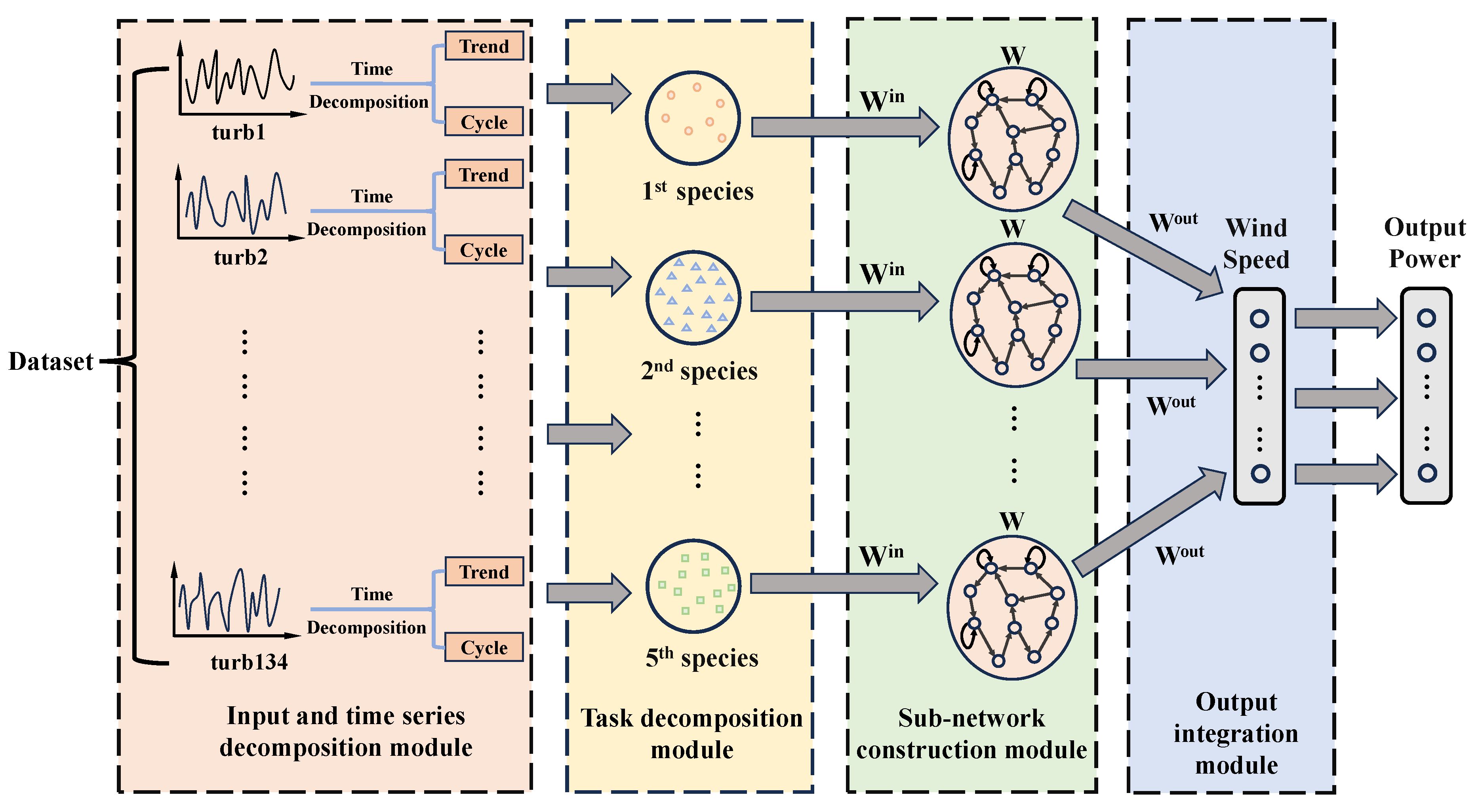
Figure 2.
The flowchart of MESN
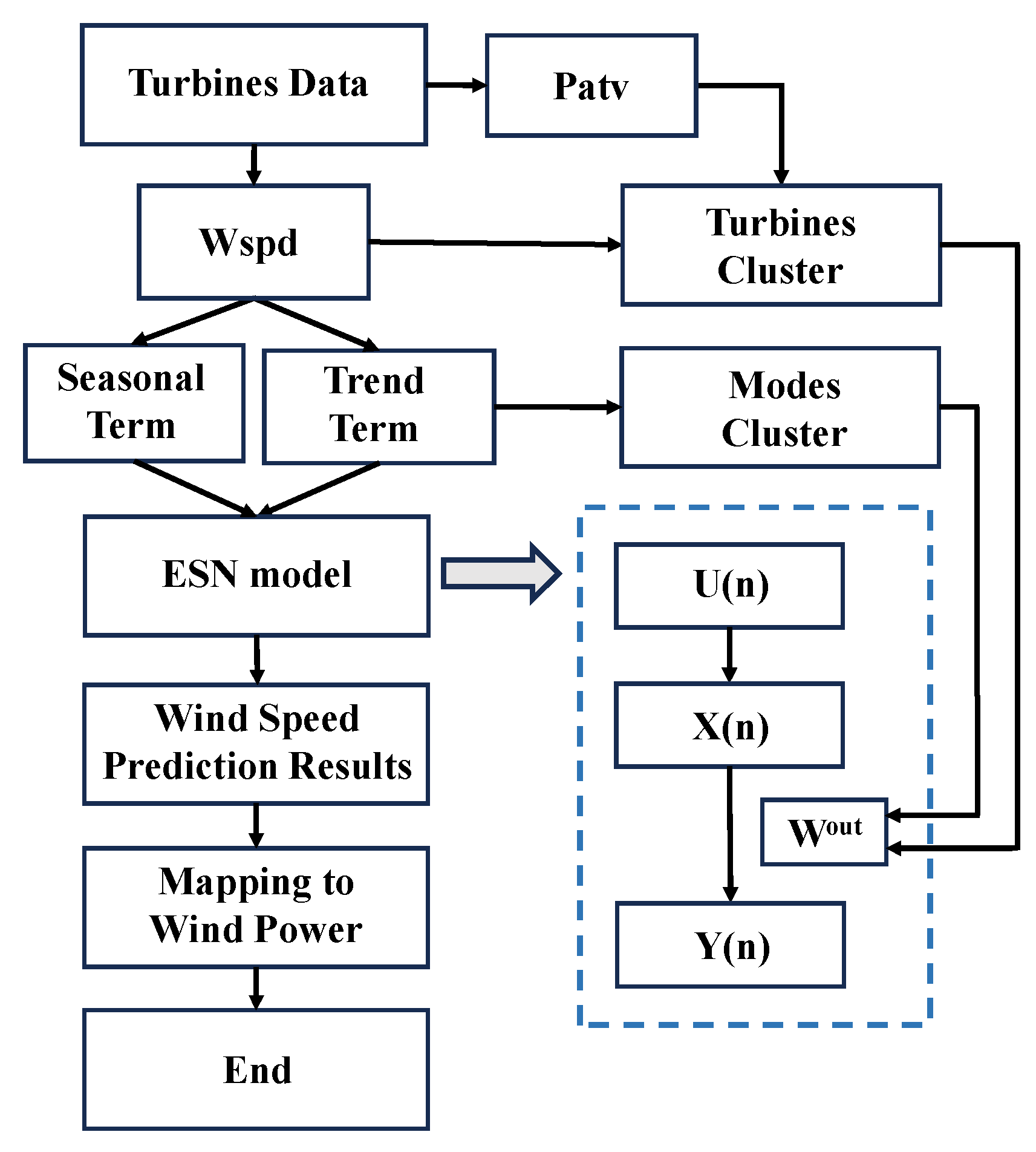
Figure 3.
Comparison chart of outlier handling based on the principles of wind turbine power generation: (a) Before outliers are handled; (b) Outliers handled.
Figure 3.
Comparison chart of outlier handling based on the principles of wind turbine power generation: (a) Before outliers are handled; (b) Outliers handled.
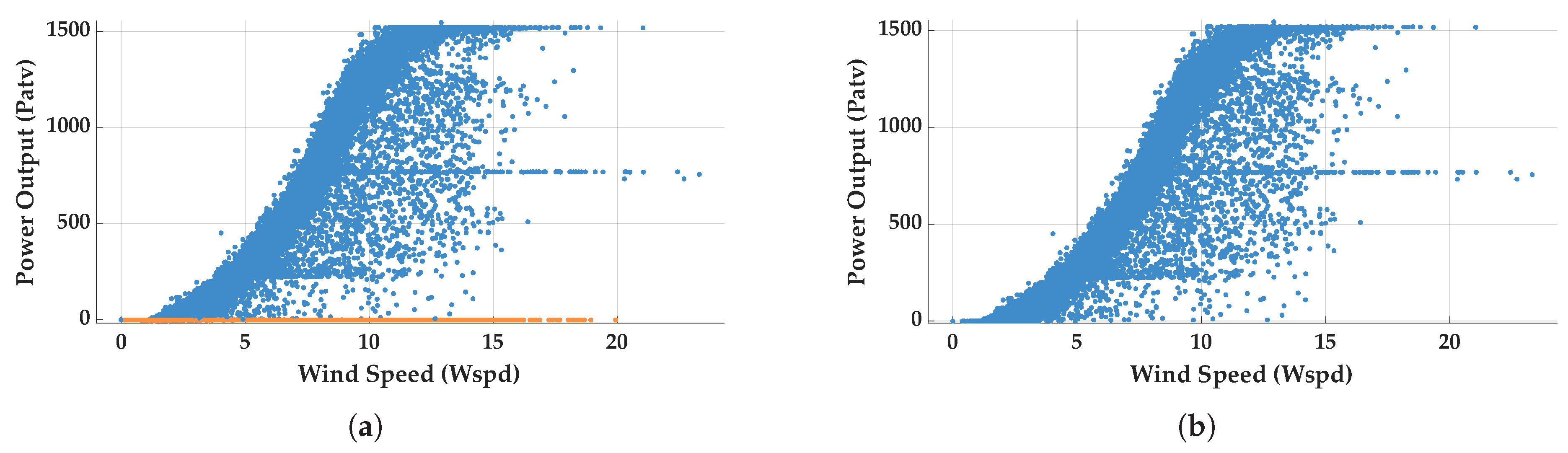
Figure 4.
Comparison of outlier handling for anomaly detection based on support vector machines: (a) Before outliers are handled; (b) Outliers handled.
Figure 4.
Comparison of outlier handling for anomaly detection based on support vector machines: (a) Before outliers are handled; (b) Outliers handled.
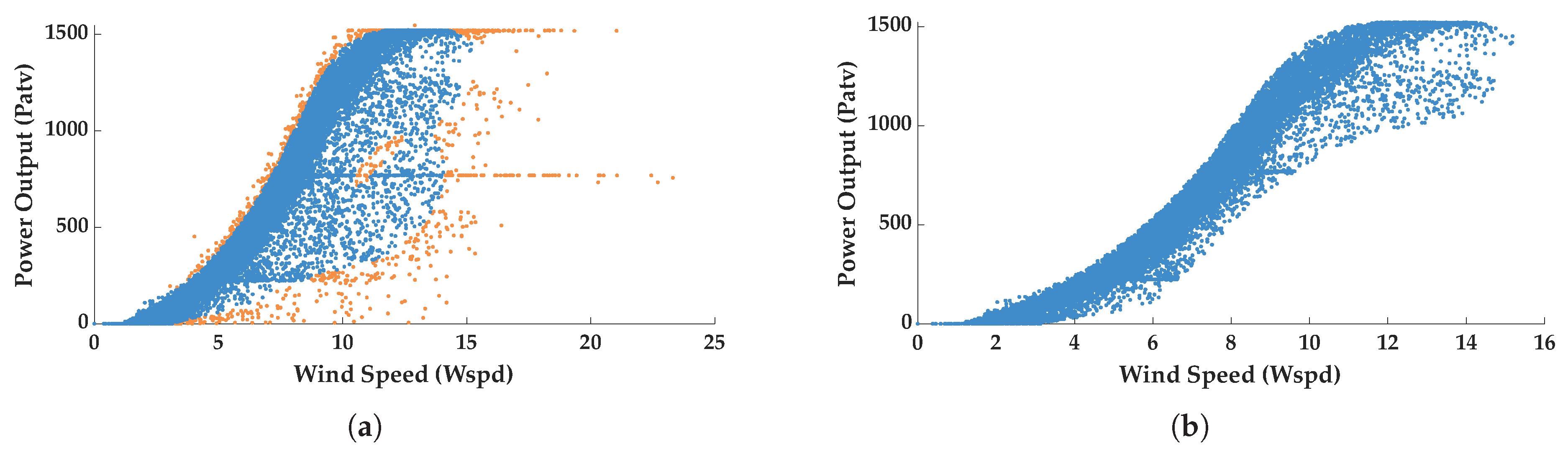
Figure 5.
The correlation coefficient between each feature of SDWPF datasets.
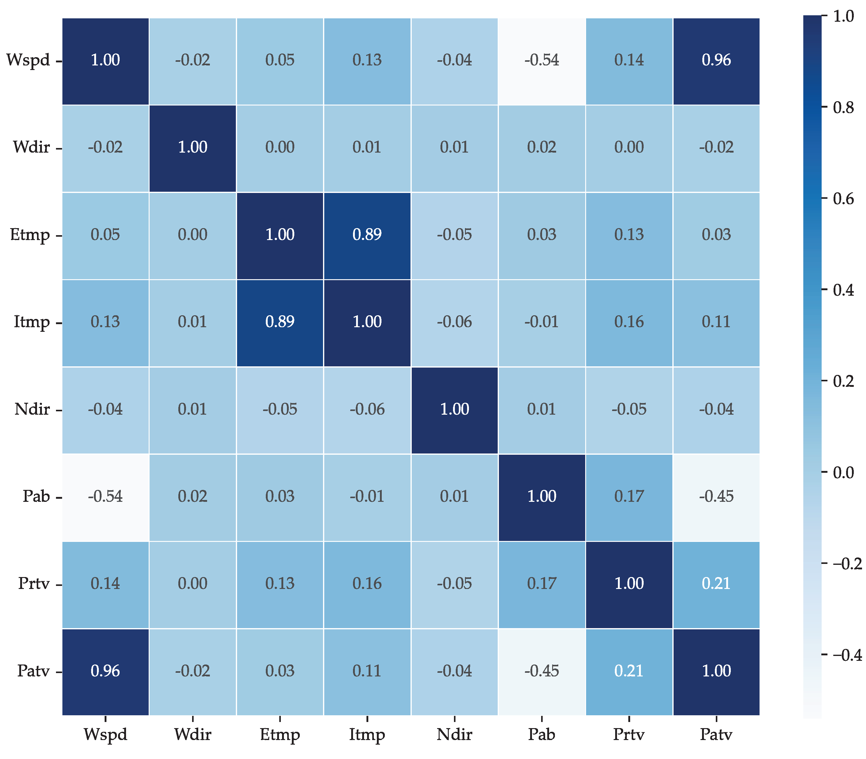
Figure 6.
Clustered Wind Speed Patterns for K=4: (a) Category 1 wind speed distribution; (b) Category 2 wind speed distribution; (c) Category 3 wind speed distribution; (d) Category 4 wind speed distribution.
Figure 6.
Clustered Wind Speed Patterns for K=4: (a) Category 1 wind speed distribution; (b) Category 2 wind speed distribution; (c) Category 3 wind speed distribution; (d) Category 4 wind speed distribution.
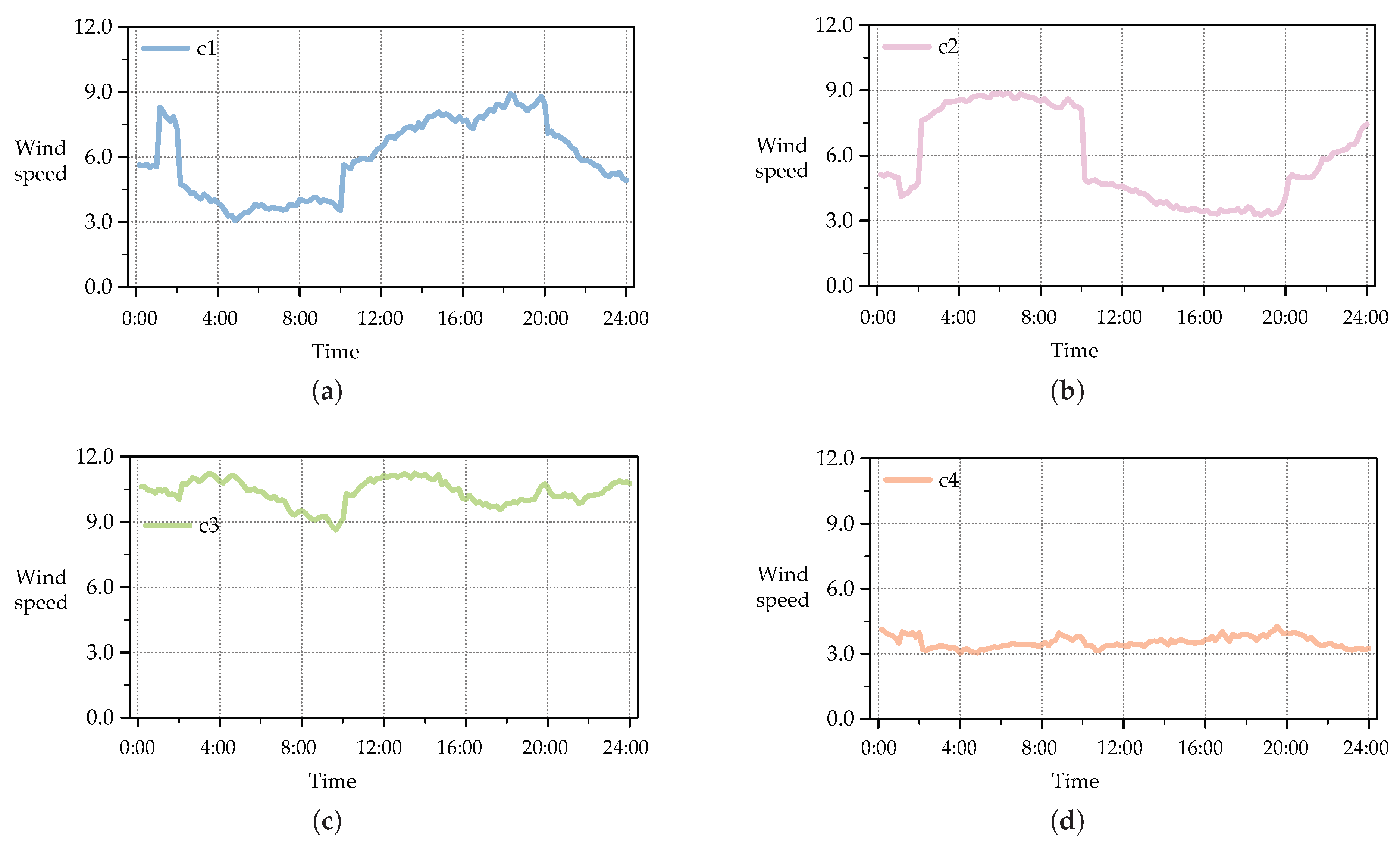
Figure 7.
Comparison of three metrics between MESN and comparative model on the test set of SDWPF datasets: (a) MSE; (b) RMSE; (c)
Figure 7.
Comparison of three metrics between MESN and comparative model on the test set of SDWPF datasets: (a) MSE; (b) RMSE; (c)
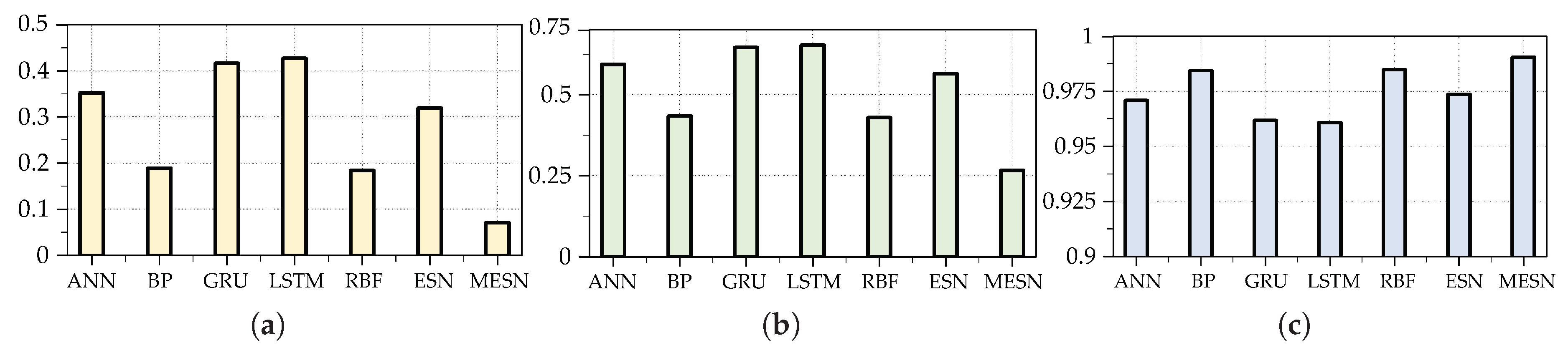
Figure 8.
Comparison of wind speed prediction data from MESN with wind speed data from the test set of SDWPF datasets.
Figure 8.
Comparison of wind speed prediction data from MESN with wind speed data from the test set of SDWPF datasets.
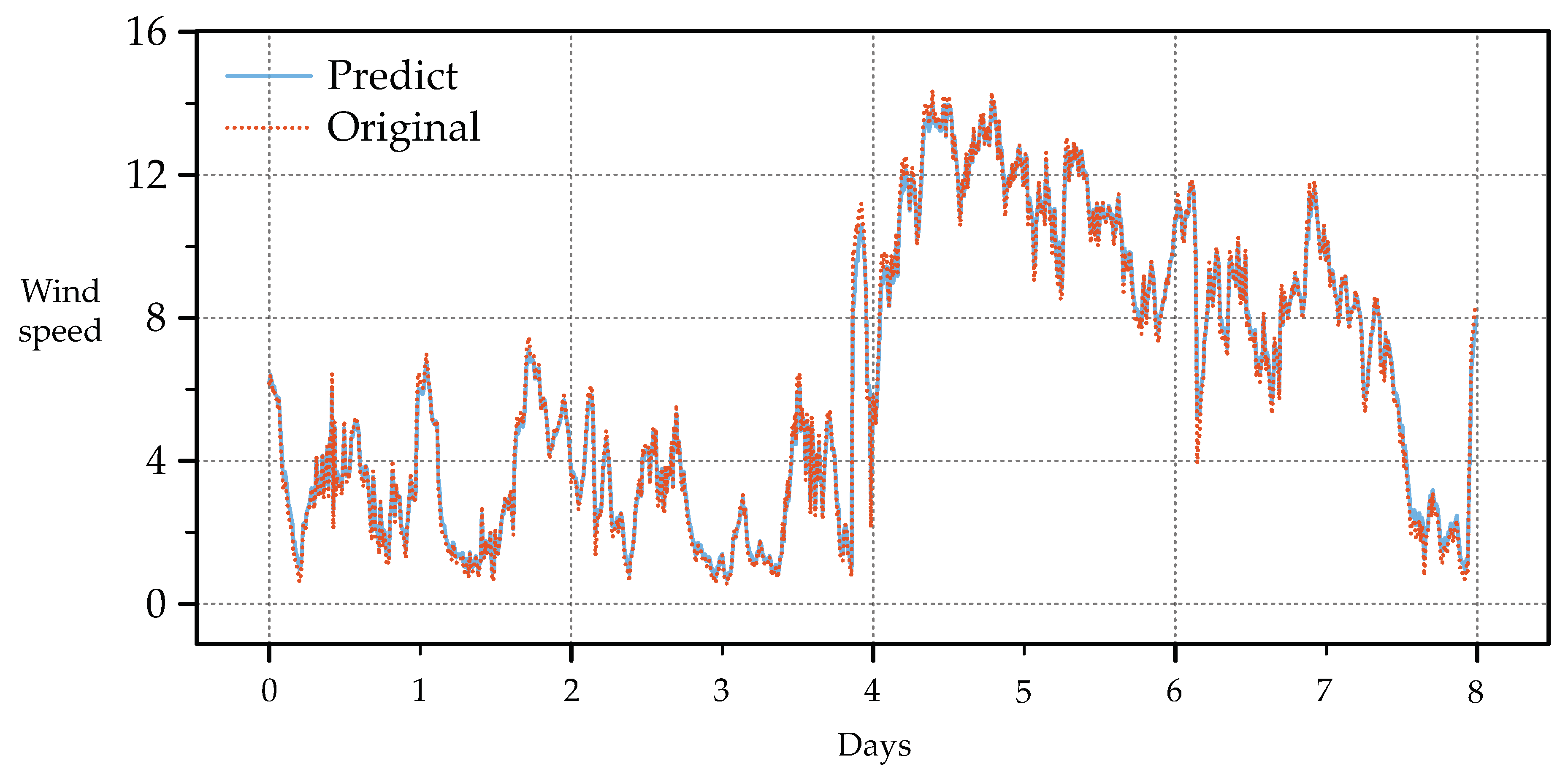
Figure 9.
Comparison of output power converted from wind speed prediction data with output power data on the test set.
Figure 9.
Comparison of output power converted from wind speed prediction data with output power data on the test set.
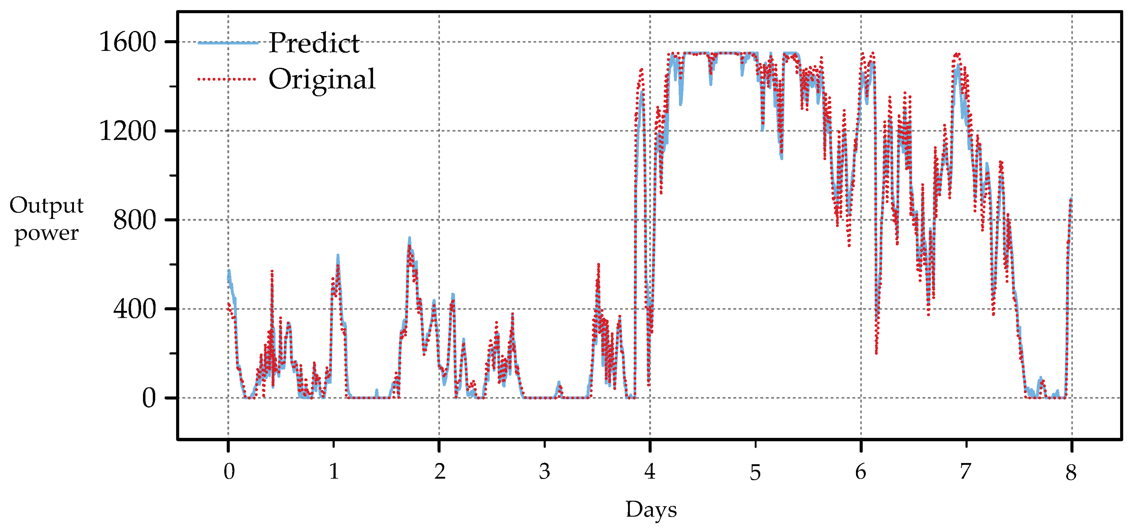

Table 1.
Feature classification and description of SDWPF datasets.
| Feature Classification | Feature Name | Feature Description |
|---|---|---|
| External features | Wspd | Wind speed recorded by an anemometer |
| External features | Wdir(°) | The angle between the wind direction and the position of the turbine generator compartment |
| External features | Etmp (°C) | Ambient temperature |
| Internal feature | Itmp (°C) | Internal temperature of turbine generator compartment |
| Internal feature | Ndir (°) | Cabin direction, i.e. the yaw angle of the cabin |
| Internal feature | Pab (°) | Pitch angle of blade |
| Power characteristics | Prtv(kW) | Reactive power |
| Power characteristics | Patv(kW) | Active power (target variable) |
Table 2.
Optimal Parameters for MESN and comparative model.
| Model | Number of layers | Number of iterations | Number of batches | Number of neuron nodes | Spectral radius | Parameters of regularization |
|---|---|---|---|---|---|---|
| ANN | 3 | 4000 | 42 | 96 | / | / |
| BP | 3 | 4200 | 42 | 96 | / | / |
| GRU | 2 | 4200 | 42 | 192 | / | / |
| LSTM | 2 | 4200 | 42 | 192 | / | / |
| RBF | / | / | / | / | 1.00E-05 | |
| ESN | / | / | / | 200 | 0.7 | 1.00E-06 |
| MESN | / | / | / | 200 | 0.8 | 1.00E-08 |
where “/” means that the corresponding parameter does not exist in the corresponding model
Table 3.
Parameter Error Statistics for MESN and comparative model
| Model | MSE | RMSE | R² |
|---|---|---|---|
| ANN | 0.3523 | 0.5936(2.23) | 0.9709 |
| BP | 0.1889 | 0.4346(1.63) | 0.9844 |
| GRU | 0.4166 | 0.6455(2.42) | 0.9617 |
| LSTM | 0.4270 | 0.6534(2.45) | 0.9607 |
| RBF | 0.1842 | 0.4292(1.61) | 0.9848 |
| ESN | 0.3194 | 0.5651(2.12) | 0.9736 |
| MESN | 0.0711 | 0.2667 | 0.9905 |
Disclaimer/Publisher’s Note: The statements, opinions and data contained in all publications are solely those of the individual author(s) and contributor(s) and not of MDPI and/or the editor(s). MDPI and/or the editor(s) disclaim responsibility for any injury to people or property resulting from any ideas, methods, instructions or products referred to in the content. |
© 2025 by the authors. Licensee MDPI, Basel, Switzerland. This article is an open access article distributed under the terms and conditions of the Creative Commons Attribution (CC BY) license (http://creativecommons.org/licenses/by/4.0/).
Copyright: This open access article is published under a Creative Commons CC BY 4.0 license, which permit the free download, distribution, and reuse, provided that the author and preprint are cited in any reuse.


