Investigation Of The Boundary Value Problem For An Extended System Of Stationary Nernst-planck-poisson Equations In The Diffusion Layer

Evgenia Kirillova; Natalia Chubyr; Roman Nazarov; Anna Kovalenko; Mahamet Urtenov

doi:10.20944/preprints202503.1371.v1

Preprint

Article

Investigation Of The Boundary Value Problem For An Extended System Of Stationary Nernst-planck-poisson Equations In The Diffusion Layer

This version is not peer-reviewed.

This version is not peer-reviewed.

Downloads

Views

Comments

Submitted:

17 March 2025

Posted:

18 March 2025

You are already at the latest version

A peer-reviewed article of this preprint also exists.

Abstract

The article investigates the boundary value problem for an extended stationary system of Nernst-Planck-Poisson equations, corresponding to a mathematical model of the influence of changes in the equilibrium coefficient on the transport of ions of a binary salt in the diffusion layer. Dimensionless variables were introduced using characteristic parameter values. As a result, a dimensionless boundary value problem was obtained, which is singularly perturbed, containing a small parameter in the derivative of the Poisson equation and, additionally, another regular small parameter. A similarity theory was developed: trivial and non-trivial similarity criteria and their physical meaning were determined, which allowed for the identification of general properties of the solutions. A numerical investigation of the boundary value problem was conducted using the finite element method. With an increase in the initial solution concentration, the value of the small parameter entering singularly decreases, reaching values on the order of 10−12 and below, leading to computational difficulties that prevent a comprehensive analysis of the influence of changes in the equilibrium coefficient on salt ion transport. In this regard, an analytical solution to the problem was constructed, based on dividing the solution domain into several subdomains (regions of electroneutrality, extended space charge region, quasi-equilibrium region, recombination region, intermediate layer), in each of which the problem is solved differently, followed by matching these solutions. Verification of the analytical solution was carried out by comparing it with the numerical solution. The advantage of the obtained analytical solution is the possibility of a comprehensive analysis of the influence of the dissociation/recombination reaction of water molecules on salt ion transport over a wide range of real changes in the concentration and composition of the electrolyte solution and other input parameters. This boundary value problem serves as a benchmark for constructing asymptotic solutions for other singularly perturbed boundary value problems in membrane electrochemistry.

Keywords:

boundary value problems

;

extended system of Nernst-Planck-Poisson equations

;

analytical solution

;

singularly perturbed problems

;

method of matched asymptotic expansions

Subject:

Computer Science and Mathematics - Applied Mathematics

MSC: 35Q92

1. Introduction

This article investigates the boundary value problem for an extended system of stationary Nernst–Planck–Poisson (NPP) equations [1,2,3,4], describing the transport of ions of a binary salt in the diffusion layer, taking into account the influence of space charge on changes in the equilibrium coefficient. This allows for a more accurate description of ion transport processes in electromembrane systems (EMS) and makes the model more universal and applicable to a wide range of parameters. Moreover, in previous works, numerical methods were generally used to solve boundary value problems in membrane electrochemistry in diffusion layers, nonlinear processes in porous electrodes, electrochemical phenomena in microfluidic systems, etc. [5,6,7,8,9,10].

The transition to dimensionless variables using characteristic parameter values shows that the boundary value problem is singularly perturbed, containing two small parameters, one of which is in the derivative of the Poisson equation, leading to computational difficulties at small parameter values in numerical solutions and the need for special methods [11,12,13]. The main problem of the analytical solution lies in the fact that different physical processes dominate in different regions of the diffusion layer [14,15]. In this article, we estimate the characteristic quantities used to make the transition to a dimensionless form, and obtain trivial and nontrivial similarity criteria. We have determined their physical meaning, defined the regions of change, and clarified the main properties of the solution to the boundary value problem. We have performed a numerical analysis of the boundary value problem and shown that the diffusion layer has a complex structure, namely, it is divided into 6 intervals where different processes dominate, and therefore, in each of them, the solution to the boundary value problem behaves differently. In this article, to construct an analytical solution to the boundary value problem, we divide the solution region into a number of subregions (regions of electroneutrality, region of extended space charge, quasi-equilibrium region, recombination region, intermediate layer), in each of which the boundary value problem is solved in its own way, and then these solutions are merged. The analytical solution is verified by comparing it with the numerical solution. The advantage of the analytical solution we obtained is the possibility of a comprehensive analysis of the effect of the dissociation/recombination reaction of water molecules on the transport of salt ions over a wide range of real changes in the concentration and composition of the electrolyte solution and other input parameters. Thus, the model we proposed and its analytical solution represent a significant step forward in understanding the processes of ion transport in EMS, taking into account the effect of the dissociation/recombination reaction of water molecules and solving boundary value problems for the extended system of NPP equations. The mathematical model we proposed and the analytical method for its study are the standard for other singularly perturbed boundary value problems in membrane electrochemistry. It demonstrates how complex physicochemical processes, such as the dissociation and recombination of water molecules [16], can be taken into account within a single mathematical formulation. This opens up new possibilities for constructing asymptotic solutions for other problems related to ion transport in EMS, when numerical methods become ineffective.

2. Mathematical Model of the Influence of the Dependence of the Dissociation Coefficient on the Space Charge Value on the Stationary Transport of Salt Ions in the Diffusion Layer

The dissociation of water at interphase boundaries and changes in the equilibrium coefficient are important for understanding the processes occurring in ion transport using ion-exchange membranes. The increase in the rate coefficient of water molecule dissociation at interphase boundaries (membrane/solution or membrane/membrane) can have several causes, as indicated in the works [17]. In this work, the influence of the electric field on the equilibrium coefficient of the water molecule dissociation/recombination reaction is investigated.

According to the concepts developed by Timashev S.F., Sheldeshov N.V. et al. [7,18,19] for bipolar membranes, the current density of

H^{+} (O H^{-})

ions generated in the membrane system is determined by an empirical formula where the equilibrium coefficient depends exponentially on the external electric field strength [7]. In electrodialysis systems with monopolar membranes, few works have been devoted to studying this dependence [20,21].

There are several considerations suggesting that, unlike the works mentioned above, in systems with monopolar membranes, changes in the equilibrium coefficient can be associated not only with the magnitude of the electric field strength but also with the magnitude of the space charge. For the first time, the dependence of

H^{+} (O H^{-})

ion fluxes on the magnitude of the space charge was mentioned in the work of Nikonenko V.V. et al. [21].

Consider the water molecule dissociation/recombination reaction equation:

\frac{d j_{H^{+}}}{d x} = \frac{d j_{O H^{-}}}{d x} = k_{r} (k_{w} - C_{H^{+}} C_{O H^{-}})

where

k_{w} = \frac{k_{d}}{k_{r}} C_{H_{2} O}

is the equilibrium constant, and

k_{d}

and

k_{r}

are the dissociation and recombination coefficients, respectively,

C_{H_{2} O}, C_{H^{+}}, C_{O H^{-}}

is the concentration of water in the solution and

H^{+} (O H^{-})

ions,

j_{H^{+}}, j_{O H^{-}}

is fluxes of

H^{+} (O H^{-})

ions. Assume that

k_{w}

depends on the space charge

ρ

. Expanding

k_{w} (ρ)

, or, what is the same

\frac{k_{d} (ρ)}{k_{r} (ρ)} = \frac{k_{d}}{k_{r}} (ρ)

, in a Taylor series with respect to

ρ

and limiting ourselves to the first approximation, we obtain the empirical formula:

\frac{k_{d}}{k_{r}} (ρ) = \frac{k_{d} (0)}{k_{r} (0)} + b ρ

, where

b

is a constant that must be determined, for example, from experimental data, considering it as a fitting parameter. We transform this formula to a convenient form by multiplying by

C_{H_{2} O}

, then

k_{w} (ρ) = \frac{k_{d}}{k_{r}} (ρ) C_{H_{2} O} = (\frac{k_{d} (0)}{k_{r} (0)} + b ρ) C_{H_{2} O} or k_{w} (ρ) = \frac{k_{d} (0)}{k_{r} (0)} C_{H_{2} O} + b C_{H_{2} O} ρ

Let us denote

k_{w_{0}} = \frac{k_{d} (0)}{k_{r} (0)} C_{H_{2} O}

and

b_{0} = b F C_{H_{2} O} = λ C_{H_{2} O}

, where

λ = b F

(

λ

is a dimensionless quantity, and, accordingly,

b_{0}

has the dimension of concentration), then we obtain

k_{w} (ρ) = k_{w_{0}} + λ \sum_{i = 1}^{n} z_{i} С_{i}

Thus, we obtain only one, dimensionless fitting parameter

λ

, which has a clear and simple physical meaning, which consists in the influence of the magnitude of the space charge on the increase in the rate of dissociation of water molecules. In addition, the function

k_{w} (ρ)

depends linearly on the values of the ion concentrations at each point, which allows us to study its change in different parts of the diffusion layer [22] and find analytical solutions.

2.1. System of Equations

Stationary transport of salt ions for a 1:1 electrolyte in a diffusion layer at a cation exchange membrane (CEM), taking into account the space charge and the dissociation/recombination reaction, taking into account the dependence of the dissociation coefficient on the value of the space charge, is described by the following extended system of NPP equations:

- \frac{d j_{i}}{d x} + R_{i} = 0, i = 1 .. 4,

(1)

j_{i} = - z_{i} \frac{F}{R T} D_{i} C_{i} \frac{d φ}{d x} - D_{i} \frac{d C_{i}}{d x},

(2)

\frac{d^{2} φ}{d x^{2}} = - \frac{ρ}{ε_{r}},

(3)

R_{3} = R_{4} = k_{d} (ρ) C_{H_{2} O} - k_{r} C_{3} C_{4} = k_{r} (k_{w} (ρ) - C_{3} C_{4}),

(4)

z_{1} = 1, z_{2} = - 1, z_{3} = 1, z_{4} = - 1,

I = F \sum_{i = 1}^{4} z_{i} j_{i},

(5)

Here (1) are the material balance equations, (2) are the Nernst-Planck equations for the flows of potassium or sodium ions (

i = 1

), chlorine (

C l^{-}, i = 2

), hydrogen (

H^{+}, i = 3

) and hydroxyl (

O H^{-}, i = 4

), (3) is the Poisson equation for the electric field potential, where

ρ = F (z_{1} C_{1} + z_{1} C_{2} + z_{3} C_{3} + z_{4} C_{4})

, (4) are the formulas describing the reaction of dissociation/recombination of water molecules, where

k_{w} (ρ) = k_{w_{0}} + b ρ

, (5) is the current flow equation, which means that the current density

I

flowing through the cross-section of the desalination channel is determined by the ion flow, that is, it is the Faraday current density,

ε_{r}

is the permittivity of the solution,

F

is the Faraday number,

R

is the universal gas constant,

T

is the absolute temperature,

ϕ

is the potential,

E = - \frac{d φ}{d x}

is the electric field strength,

C_{i}

j_{i}

D_{i}

– is the concentration, flux, diffusion coefficient of the i-th ion,

k_{r} (0) = 1, 1 \cdot 10^{8}

m³ /(s mol) is the recombination rate constant,

k_{d} (0) = 2 \cdot 10^{- 5}

s⁻¹ is the dissociation rate constant of water molecules,

k_{w_{0}} = \frac{k_{d}}{k_{r}} (0) C_{H_{2} O} = 10^{- 8}

mol² /m⁶ is the equilibrium coefficient (ionic product of water).

Remark 1.

As follows from equations (1) and formulas (4), (5), the relations

z_{1} j_{1} + z_{2} j_{2} = \frac{I_{s}}{F}

z_{3} j_{3} + z_{4} j_{4} = \frac{I_{w}}{F}

and

I = I_{s} + I_{w}

are valid, where

I_{s}, I_{w}

are constant unknown partial currents for salt ions and dissociation products of water molecules.

2.2. Boundary Conditions

x = 0

C_{1} (0) = C_{10},

(6)

C_{2} (0) = C_{20},

(7)

C_{3} (0) = C_{30}, C_{30} > > \sqrt{k_{w_{0}}},

(8)

C_{4} (0) = k_{w_{0}} / C_{30},

(9)

φ (0) = d .

(10)

The concentration values are considered to be known and given (6), (7), (8), Condition (8) means that the solution away from the cation exchange membrane is acidified.

x = h

C_{1} (h) = C_{1 K},

(11)

{(\frac{F}{R T} D_{2} C_{2} \frac{d φ}{d x} - D_{2} \frac{d C_{2}}{d x}) |}_{x = h} = 0,

(12)

\frac{d C_{3} (h)}{d x} = 0,

(13)

{(\frac{F}{R T} C_{4} D_{4} \frac{d φ}{d x} - D_{4} \frac{d C_{4}}{d x}) |}_{x = h} = j_{4 k},

(14)

φ (h) = 0 .

(15)

The concentration of cations (11) on the membrane surface is determined by its exchange capacity, and the membrane is considered to be ideally selective (12). It is believed that in the surface layer of the cation-exchange membrane there is a less intense generation of

H^{+} (O H^{-})

than in the anion-exchange membrane, therefore the concentration of

H^{+}

ions is significantly less than the concentration of cations, and they pass through the membrane freely (13) and no longer participate in the transport processes. In this case, a flow of

O H^{-}

ions is injected into the solution from the surface of the cation-exchange membrane and this flow is specified by condition (14). In this study, the potential drop (10), (15) is specified and the current density is found using formula (5).

3. Trivial and Non-Trivial Similarity Criteria

3.1. Characteristic Quantities and Transition to Dimensionless Form

Let us take the initial concentration C₀ of the solution as a characteristic concentration, and the actual values of the solution as a characteristic concentration, and the actual values C₀ are in the range 10⁻³M–100M. Let us consider the thickness of the diffusion layer

h

, which has the order of

10^{- 4} m

[23], as a characteristic length. Let us denote

D_{0} = \frac{2 D_{1} \cdot D_{2}}{D_{1} + D_{2}}

– the diffusion coefficient of the electrolyte, for example, (NaCl), (

D_{0} = 1, 6133 \cdot 10^{- 9} m^{2} / s

);

ϕ_{0} = \frac{R T}{F}

– the thermal potential (

ϕ_{0} = 0, 026 В

) [2].

Let us introduce the limiting diffusion current according to the formula [24]

I_{n p} = \frac{2 D_{1} C_{0} F}{h}

Let's take

I_{0} = \frac{I_{n p}}{2}

I_{0}

. Let us estimate the value

I_{0}

, which depends on the initial concentration

I_{0} = [C_{0}] \cdot 0, 649 \cdot \frac{А}{m^{2}}

, for example, at

C_{0} = 1 \frac{m o l}{m^{3}}

, we obtain

I_{0} = 0, 649 \cdot \frac{А}{m^{2}}

Let us move on to dimensionless quantities using the following formulas:

x^{(u)} = \frac{x}{h}, φ^{(u)} = \frac{φ}{φ_{0}}, E^{(u)} = - \frac{h}{ϕ_{0}} \frac{d ϕ}{d x}, I^{(u)} = \frac{I}{I_{0}}, D_{i}^{(u)} = \frac{D_{i}}{D_{0}}, C_{i}^{(u)} = \frac{C_{i}}{C_{0}}, j_{i}^{(u)} = \frac{j_{i} h}{D_{i} C_{0}} = \frac{j_{i} F}{D_{i}^{(u)} I_{0}}, i = 1, ..., 4 .

Then we obtain the boundary value problem in dimensionless form:

ε^{(u)} D_{i}^{(u)} \frac{d j_{i}^{(u)}}{d x^{(u)}} = a^{(u)} (k_{w_{0}}^{(u)} + β (C_{1}^{(u)} - C_{2}^{(u)} + C_{3}^{(u)} - C_{4}^{(u)}) - C_{3}^{(u)} C_{4}^{(u)}), ε^{(u)} \frac{d^{2} ϕ^{(u)}}{d {(x^{(u)})}^{2}} = - (С_{1}^{(u)} - С_{2}^{(u)} + С_{3}^{(u)} - С_{4}^{(u)}), j_{i}^{(u)} = - z_{i} C_{i}^{(u)} \frac{d φ^{(u)}}{d x^{(u)}} - \frac{d C_{i}^{(u)}}{d x^{(u)}}, I^{(u)} = \sum_{i = 1}^{4} z_{i} D_{i}^{(u)} j_{i}^{(u)}, I_{s}^{(u)} = D_{1}^{(u)} j_{1}^{(u)} - D_{2}^{(u)} j_{2}^{(u)}, I_{w}^{(u)} = D_{3}^{(u)} j_{3}^{(u)} - D_{4}^{(u)} j_{4}^{(u)} .

The boundary conditions are as follows:

x = 0

C_{1}^{(u)} (0) = C_{10}^{(u)},

C_{2}^{(u)} (0) = C_{20}^{(u)},

C_{3}^{(u)} (0) = C_{30}^{(u)}, C_{30}^{(u)} > > \sqrt{k_{w_{0}}},

C_{4}^{(u)} (0) = k_{w_{0}} / C_{30}^{(u)},

C_{10}^{(u)} - C_{20}^{(u)} + C_{30}^{(u)} - C_{40}^{(u)} = 0, ϕ^{(u)} (1) = d .

x = 1

C_{1}^{(u)} (1) = C_{1 m},

{(C_{2}^{(u)} \frac{d ϕ^{(u)}}{d x^{(u)}} - \frac{d C_{2}^{(u)}}{d x^{(u)}}) |}_{x = 1} = 0,

\frac{d C_{3}^{(u)} (1)}{d x^{(u)}} = 0,

D_{4} {(C_{4}^{(u)} \frac{d ϕ^{(u)}}{d x^{(u)}} - \frac{d C_{4}^{(u)}}{d x^{(u)}}) |}_{x = 1} = j_{4 k},

ϕ^{(u)} (1) = 0 .

3.2. Physical Meaning of Similarity Criteria

The boundary value problem contains the following parameters

ε^{(u)}, D_{3}^{(u)}, D_{4}^{(u)}, a^{(u)}, k^{(u)}, {\bar{k}}_{w}^{(u)}, β^{(u)}, b^{(u)}

, which are trivial similarity criteria. Let us determine the physical meaning of these parameters and estimate their values at characteristic values of the input parameters of the problem.

1): Let's consider the parameter $ε^{(u)}$ .

Let us find out the physical meaning of this parameter. To do this, we write it in the form,

ε^{(u)} = \frac{R T_{0} ε_{r}}{C_{0} F^{2} h^{2}} = 2 {(\frac{l_{d}}{h})}^{2}

, where

l_{d} = \sqrt{\frac{R T ε_{r}}{2 C_{0} F^{2}}}

is the Debye length.

Thus, the parameter

ε^{(u)}

is the doubled square of the ratio of the Debye length

l_{d}

to the width of the diffusion layer

h

, i.e.

\sqrt{ε^{(u)}}

is the dimensionless Debye length (the thickness of the quasi-equilibrium region of the space charge)

The estimate

ε^{(u)}

shows that

1.859 \times 10^{- 12} \leq ε^{(u)} \leq 1.859 \times 10^{- 8}

. As can be seen from the value

ε^{(u)}

, it can be taken as a small parameter, and with an increase in the initial concentration of the solution

С_{0}

, its value decreases.

2): Let us consider the parameter $k_{w_{0}}^{(u)} = \frac{k_{d} C_{H_{2} O}}{k_{r} C_{0}^{2}}$ .

The estimate

k_{w_{0}}^{(u)}

shows that it varies within

10^{- 14} \leq k_{w_{0}}^{(u)} \leq 10^{- 6}

. So, for example, for

С_{0} = 1

mol/m³ we have

k_{w_{0}}^{(u)} \approx 10^{- 8}

It is clear that

k_{w_{0}}^{(u)}

can be considered as a small parameter, independent of

ε^{(u)}

, and with an increase in the initial concentration of the solution

С_{0}

, it decreases rapidly.

However, if the width of the diffusion layer is fixed, then there is a relationship between them (see below).

3): Consider the parameter $a^{(u)}$

a^{(u)} = \frac{k_{r} ϕ_{0} ε_{r}}{D_{0} F} = 12.6

- a universal constant independent of the initial concentration, potential jump, etc. To clarify the physical meaning of this parameter, we transform it as follows:

a^{(u)} = \frac{k_{r} R T ε_{r}}{D_{0} F^{2}} = \frac{2 C_{0} k_{r} R T ε_{r}}{D_{0} 2 C_{0} F^{2}} = \frac{2 C_{0} k_{r} l_{d}^{2}}{D_{0}} = \frac{l_{d}^{2}}{\frac{D_{0}}{2 C_{0} k_{r}}} = \frac{l_{d}^{2}}{l_{r}^{2}}

where

l_{r} = \sqrt{\frac{D_{0}}{2 C_{0} k_{r}}}

is the width of the recombination region. For example, for

С_{0} = 1

mol/m³ we have .

Thus, the parameter

a^{(u)}

is the square of the ratio of the Debye length

l_{d}

to the width of the recombination region

l_{r}

. The value of the constant

a^{(u)} = 12, 6

shows that the recombination region is approximately 3,5 times smaller than the quasi-equilibrium region of the space charge.

4): Let the width of the diffusion layer be fixed, then we have the following non-trivial similarity criterion $k_{w_{0}} = B ε^{2}$ , where

B^{(u)} = \frac{k_{d} C_{H_{2} O} F^{2} h^{4}}{k_{r} {(ε_{r})}^{2} {(ϕ_{0})}^{2}} = 2, 86 \cdot 10^{11}

is a dimensionless parameter.

In addition,

R_{3}^{(u)} = R_{4}^{(u)} = \frac{a^{(u)}}{ε^{(u)}} (B^{(u)} {(ε^{(u)})}^{2} - C_{3}^{(u)} C_{4}^{(u)})

k_{w_{0}} = B ε^{2}

follows that with an increase in the initial concentration of the solution

С_{0}

, the influence of the dissociation/recombination reaction on the transfer of salt ions rapidly decreases.

4. Analysis of Numerical Solution and Algorithm of Analytical Solution

We have developed a special program "Program for computer modeling of changes in the rate constant of dissociation and recombination of water molecules in the diffusion layer" №2024688199 in the Comsol MPh 6.2 environment. With the help of which we carried out a numerical study of the boundary value problem using the finite element method. This software product is designed to calculate the mathematical model (1-15) and allows to describe with high accuracy the processes occurring in the diffusion layer of ion-exchange membranes, taking into account the reactions of dissociation and recombination of water molecules. This program provides a more adequate idea of the behavior of salt ions under steady-state transfer conditions, which can be used to develop new materials and technologies for ion-exchange membranes with improved characteristics, with increased selectivity, strength and resistance to various effects. The functionality of the program includes input of initial data, calculation of the mathematical model and visualization of the results on graphs (Figure 2, Figure 3 and Figure 4), surfaces and video, comparison with the analytical solution.

An analysis of the numerical solution shows that the diffusion layer can be conditionally divided into six intervals by five points:

x_{r}

- the center of the recombination region

(x_{r} - δ_{1}, x_{r} + δ_{1})

x_{с}

- the center of the intermediate region

(x_{с} - δ_{2}, x_{с} + δ_{2})

between the region of electroneutrality

(x_{r} + δ_{1}, x_{c} - δ_{2})

and the region of extended space charge

(x_{с} + δ_{2}, x_{q})

, where the space charge has a local maximum,

x_{q}

- the left boundary of the quasi-equilibrium region of space charge (Figure 1).

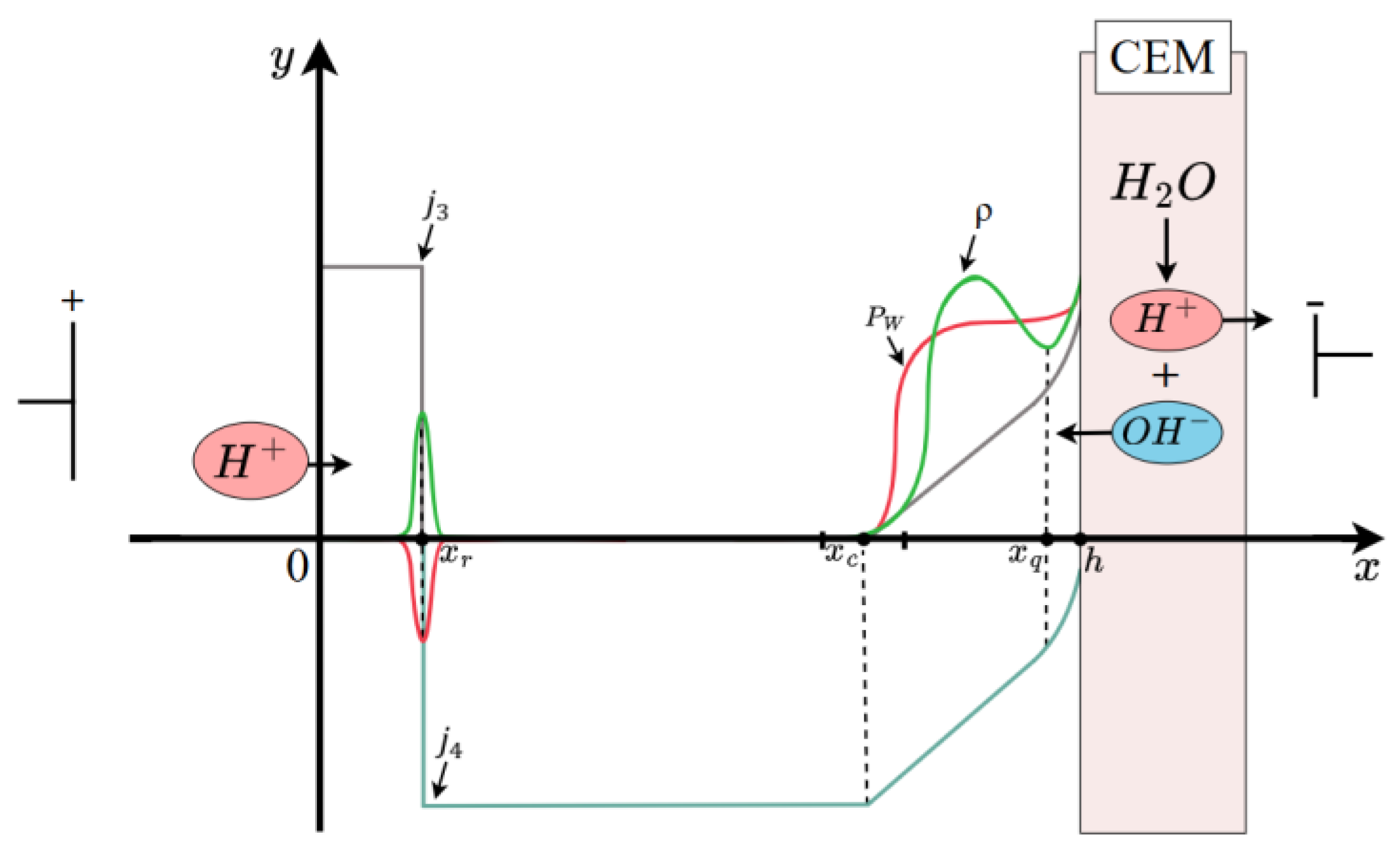
Figure 1. Diagram of the structure of the diffusion layer in a cation exchange membrane (CEM). Not to scale.

In the region

(0, x_{r} - δ_{1})

, the equilibrium is shifted (the solution is acidified) due to the generation of

H^{+}

ions (see the boundary condition). In this region, there are practically no

O H^{-}

ions (the concentration of these ions is significantly less than the concentration of

H^{+}

ions). The concentration of cations and anions is equal with high accuracy, even if they are artificially set unequal at

x = 0

, this inequality is compensated for on the artificially arising boundary layer. In the region

[0, x_{r} - δ_{1})

, the value of the space charge is sufficiently small and, as a first approximation, it can be assumed that the condition of local electroneutrality is satisfied in it (Figure 2).

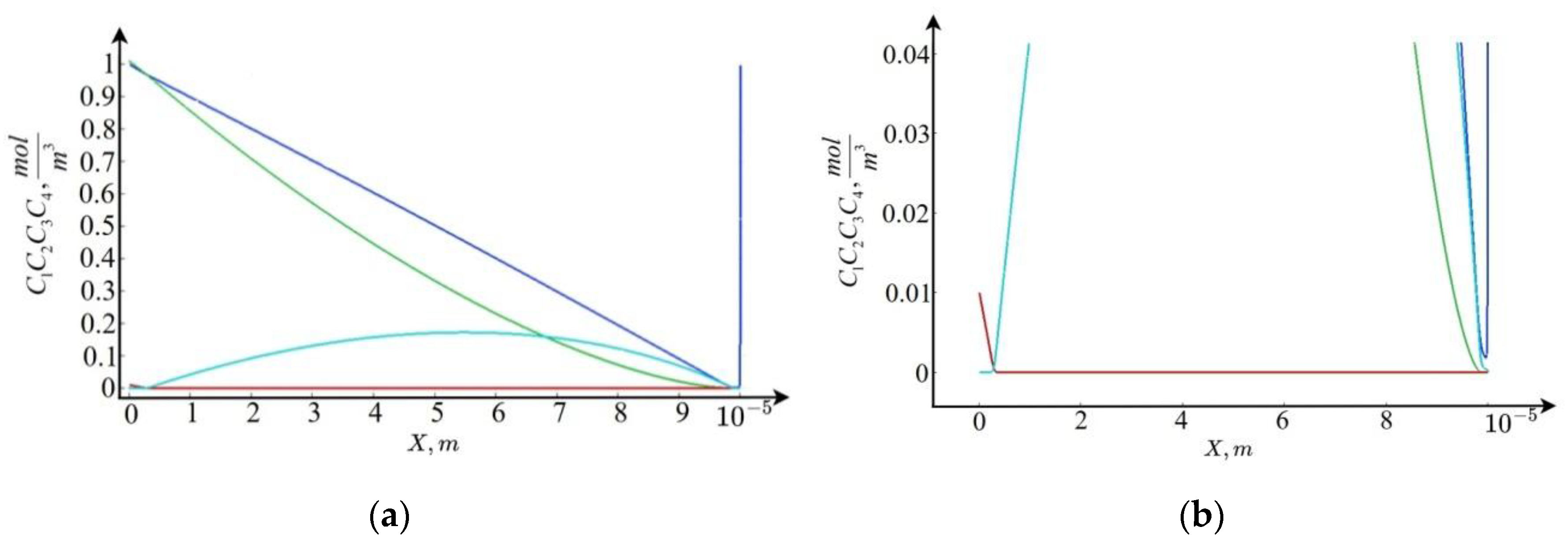
Figure 2. Concentration graphs. Blue –concentration graph, green –

C l^{-}

, red –

H^{+}

, light blue –

O H^{-}

: (a) general view, (b) enlargement.

Figure 2. Concentration graphs. Blue –concentration graph, green –

C l^{-}

, red –

H^{+}

, light blue –

O H^{-}

: (a) general view, (b) enlargement.

On the segment

(x_{r} - δ_{1}, x_{r} + δ_{1})

, there is a recombination of hydrogen ions that come from the depth of the solution towards the cation exchange membrane with hydroxyl ions that arise in the space charge region (SCR) of the cation exchange membrane. In this region, the recombination of

H^{+}

and

О H^{-}

ions dominates over the dissociation reaction of water molecules, so we will call this region the recombination region. On the interval

(x_{с} - δ_{2}, 1]

, the condition of local electroneutrality is violated, that is, this space charge region, and the interval

(x_{с} + δ_{2}, x_{q})

is an extended space charge region that occurs at currents above the limiting value,

(x_{с} - δ_{2}, x_{с} + δ_{2})

is an intermediate layer between the electroneutrality region and the extended SCR, and the interval

(x_{q}, 1]

is a quasi-equilibrium space charge region. On each interval, the solution is sought in its own way, and then they are merged, that is, the constants included in the solution are determined and the boundaries of the intervals are specified. Let us note some properties of the solutions. From the numerical analysis (Figure 2) and asymptotic estimates it follows that the cation concentration

С_{1}

changes linearly on the interval

[0, x_{с} - δ_{2})

, then slowly decreases to the point

x_{q}

, and then, exponentially increasing, satisfies the boundary condition

C_{1} (1) = C_{1 k}

at the point

x = 1

. The anion concentration

С_{2}

decreases linearly on the interval

[0, x_{с} - δ_{2})

, and then becomes practically equal to zero. The ion concentration

H^{+}

decreases linearly on the interval

[0, x_{r} + δ_{1})

, then the concentration value is practically equal to zero up to the point

x_{с}

, after which it begins to grow, reaching a local maximum at the point

x_{q}

, and then decreases. The ion concentration

О H^{-}

on the interval

[0, x_{r} - δ_{1})

is practically equal to zero, then this concentration begins to grow, reaching its maximum at some internal point

(x_{r}, x_{c})

, and then the concentration on the interval

(x_{q}, 1]

becomes practically equal to zero.

5. Analytical Solution

For the convenience of the analytical solution, we write a dimensionless boundary value problem, omitting the index "u" for simplicity of notation:

ε D_{i} \frac{d j_{i}}{d x} = a (k_{w_{0}} + β (C_{1} - C_{2} + C_{3} - C_{4}) - C_{3} C_{4}), i = 3, 4

(16)

ε \frac{d^{2} ϕ}{d x^{2}} = - (C_{1} - C_{2} + C_{3} - C_{4}),

(17)

j_{i} = - z_{i} C_{i} \frac{d ϕ}{d x} - \frac{d C_{i}}{d x}, i = 1, 2, 3, 4

(18)

I = \sum_{i = 1}^{4} z_{i} D_{i} j_{i},

(19)

I_{s} = D_{1} j_{1} - D_{2} j_{2}, I_{w} = D_{3} j_{3} - D_{4} j_{4} .

x = 0

C_{1} (0) = 1, C_{2} (0) = 1,

C_{3} (0) = C_{30}, C_{30} > > \sqrt{k_{w_{0}}},

C_{4} (0) = k_{w_{0}} / C_{30},

C_{3} (0) = 1,

C_{10} - C_{20} + C_{30} - C_{40} = 0, ϕ (1) = d .

x = h

C_{1} (1) = C_{1 m},

{(C_{2} \frac{d ϕ}{d x} - \frac{d C_{2}}{d x}) |}_{x = 1} = 0,

\frac{d C_{3} (1)}{d x} = 0,

D_{4} {(C_{4} \frac{d ϕ}{d x} - \frac{d C_{4}}{d x}) |}_{x = 1} = j_{4 k},

ϕ (1) = 0 .

The system of equations contains two small parameters

ε

and

k_{w_{0}}

, and the parameter

ε

enters the equations singularly, i.e. as a coefficient at the derivative, and the parameter

k_{w_{0}}

is regular [25,26], therefore the system of equations is simultaneously singularly and regularly perturbed.

General idea of the solution.

We divide the initial segment into six intervals:

[0, 1] = [0, x_{r} - δ_{1}) \cup [x_{r} - δ_{1}, x_{r} + δ_{1}) \cup [x_{r} + δ_{1}, x_{c} - δ_{2}) \cup [x_{с} - δ_{2}, x_{с} + δ_{2}) \cup [x_{с} + δ_{2}, x_{q}) \cup [x_{q}, 1] .

In each interval, the system of equations is simplified in its own way and a general solution is found. The constants of integration and the boundaries of the intervals are found from the condition of matching the solutions at the boundaries of the intervals.

In the intervals

[0, x_{r} - δ_{1})

[x_{r} + δ_{1}, x_{c} - δ_{2})

, in the first approximation, the condition of electroneutrality and equilibrium is satisfied, therefore we obtain the equations:

k_{w_{0}} - C_{3} C_{4} = 0

i = 3, 4

C_{1} - C_{2} + C_{3} - C_{4} = 0

\frac{d C_{i}}{d x} = - z_{i} C_{i} \frac{d ϕ}{d x} - j_{i}

i = 1, 2, 3, 4

where the flows are constant, and in

[0, x_{r} - δ_{1})

we have

j_{3} \approx \frac{I_{w}}{D_{3}}, j_{4} \approx 0

, and in

[x_{r} + δ_{1}, x_{c} - δ_{2})

, on the contrary,

j_{4} \approx - \frac{I_{w}}{D_{4}}, j_{3} \approx 0

The general solutions of these equations are found quite simply and therefore omitted here.

5.1. Analytical Solution in the Recombination Region $[x_{r} - δ_{1}, x_{r} + δ_{1})$

In the recombination region, the equilibrium is disturbed. In the first approximation, the condition of local electroneutrality is satisfied, however, in this interval

C_{1} - C_{2} + C_{3} - C_{4} = O (\sqrt{ε)}

, unlike

C_{1} - C_{2} + C_{3} - C_{4} = O (ε)

in the interval

[x_{r} + δ_{1}, x_{c} - δ_{2})

From asymptotic estimates, numerical solution and physical considerations, the following assumptions are valid:

1): the width of the recombination region is small (i.e., $δ_{1}$ is small);
2): recombination prevails over dissociation, i.e. $k_{w_{0}} < < C_{3} C_{4}$ , in $(x_{r} - δ_{1}, x_{r})$ $C_{4} \approx 0$ , and in $(x_{r}, x_{r} + δ_{1})$ $C_{3} \approx 0$ .

Using these assumptions, the system of equations (16)-(19) is simplified:

ε D_{i} \frac{d j_{i}}{d x} = a (k_{w_{0}} - C_{3} C_{4}), i = 3, 4

(20)

C_{1} - C_{2} + C_{3} - C_{4} = 0,

(21)

j_{i} = - z_{i} C_{i} \frac{d ϕ}{d x} - \frac{d C_{i}}{d x}, i = 1, 2, 3, 4

(22)

I = \sum_{i = 1}^{4} z_{i} D_{i} j_{i},

(23)

I_{s} = D_{1} j_{1} - D_{2} j_{2}, I_{w} = D_{3} j_{3} - D_{4} j_{4} .

From this system, after a number of transformations, we obtain the equation for

j_{3}

\frac{ε D_{3} D_{4}}{a} \frac{d^{2} j_{3}}{d x^{2}} = (D_{4} C_{4} + D_{3} C_{3}) j_{3} - C_{3} I_{w} .

(24)

Remark 2.

If we formally put in equation (24)

ε = 0

, we obtain the equation

(D_{4} C_{4} + D_{3} C_{3}) j_{3} - C_{3} I_{w} = 0

, whence, taking into account

C_{4} \approx 0

, we obtain

j_{3} \approx \frac{I_{w}}{D_{3}}

and

j_{4} \approx 0

. That is, the assumptions used for the solution in the interval

[0, x_{r} - δ_{1})

. Similarly, if we put

C_{3} \approx 0

, we get

j_{3} \approx 0

. That is, the assumptions used for the solution in the interval

(x_{r} + δ_{1}, x_{c} - δ_{2})

. This allows us to merge solutions in all three intervals.

1): Let's find a solution in the interval $(x_{r} - δ_{1}, x_{r}]$

Taking into account

C_{4} (x) \approx 0

we get a linear non-homogeneous equation of the second order:

\frac{ε D_{3} D_{4}}{a} \frac{d^{2} j_{3}}{d x^{2}} = D_{3} C_{3} (x) j_{3} - C_{3} (x) I_{w}

After a series of transformations, we get an approximate analytical solution:

j_{3} (x, ε) = А_{2} \exp (- \sqrt{a \frac{С_{3} (x_{r})}{D_{4}}} \frac{x_{r} - x}{\sqrt{ε}}) + \frac{I_{w}}{D_{3}}

, where

A_{2}

is the constant of integration

Let's find the value

j_{3} (x, ε)

at the point

x_{r} - δ_{1}

. The first term, regardless of

A_{2}

, should be close to zero. If we take

x = x_{r} - δ_{1}

, where

δ_{1} = - k \sqrt{ε} \ln ε

, where

k > 0

is an arbitrary constant, we get that by choosing

k

we can ensure proximity

j_{3} (x_{r} - δ_{1})

\frac{I_{w}}{D_{3}}

with any degree of

ε

. Note that

j_{3} (x_{r}, ε) = А_{2} + \frac{I_{w}}{D_{3}}

2): Let's find the solution in the interval $[x_{r}, x_{r} + δ_{1})$

Similarly to item 1), we find the solution in the interval

[x_{r}, x_{r} + δ_{1})

, using the equation

\frac{ε D_{3} D_{4}}{a} \frac{d^{2} j_{3}}{d x^{2}} = D_{4} C_{4} (x) j_{3}

j_{3} (x, ε) = B_{2} \exp (- \sqrt{a \frac{С_{4} (x_{r})}{D_{3}}} \frac{x - x_{r}}{\sqrt{ε}})

, where

B_{2}

is the constant of integration.

To merge the solutions

(x_{r} - δ_{1}, x_{r}]

and

[x_{r}, x_{r} + δ_{1})

, the condition of continuity and smoothness of the function

j_{3} (x, ε)

at the point

x_{r}

is used, which gives a system of equations that uniquely determines

А_{2}, B_{2}

А_{2} + \frac{I_{w}}{D_{3}} = B_{2}

and

А_{2} \sqrt{a \frac{С_{3} (x_{r})}{D_{4} ε}} = - B_{2} \sqrt{a \frac{С_{4} (x_{r})}{D_{3} ε}}

3): Making calculations similar to 1) and 2), it is easy to find $j_{4} (x, ε)$ and show that the relation is satisfied $D_{3} j_{3} (x, ε) - D_{4} j_{4} (x, ε) = I_{w}$ in the entire recombination region. In addition, from the solutions given above, it follows that the width of the recombination region is of the order of $O (\sqrt{ε} \ln ε)$ .

5.2. Analytical Solution in the Extended RPR

We present the solution in the extended region of space charge

(x_{c} + δ_{2}; x_{q})

. As follows from the analysis of the numerical solution in this region and the asymptotic estimates, dissociation dominates over recombination, and

C_{1}

slowly decreases, and is of the order of

C_{1} = O (\sqrt{ε})

C_{1} > C_{4} > > C_{3},

C_{2} \approx 0

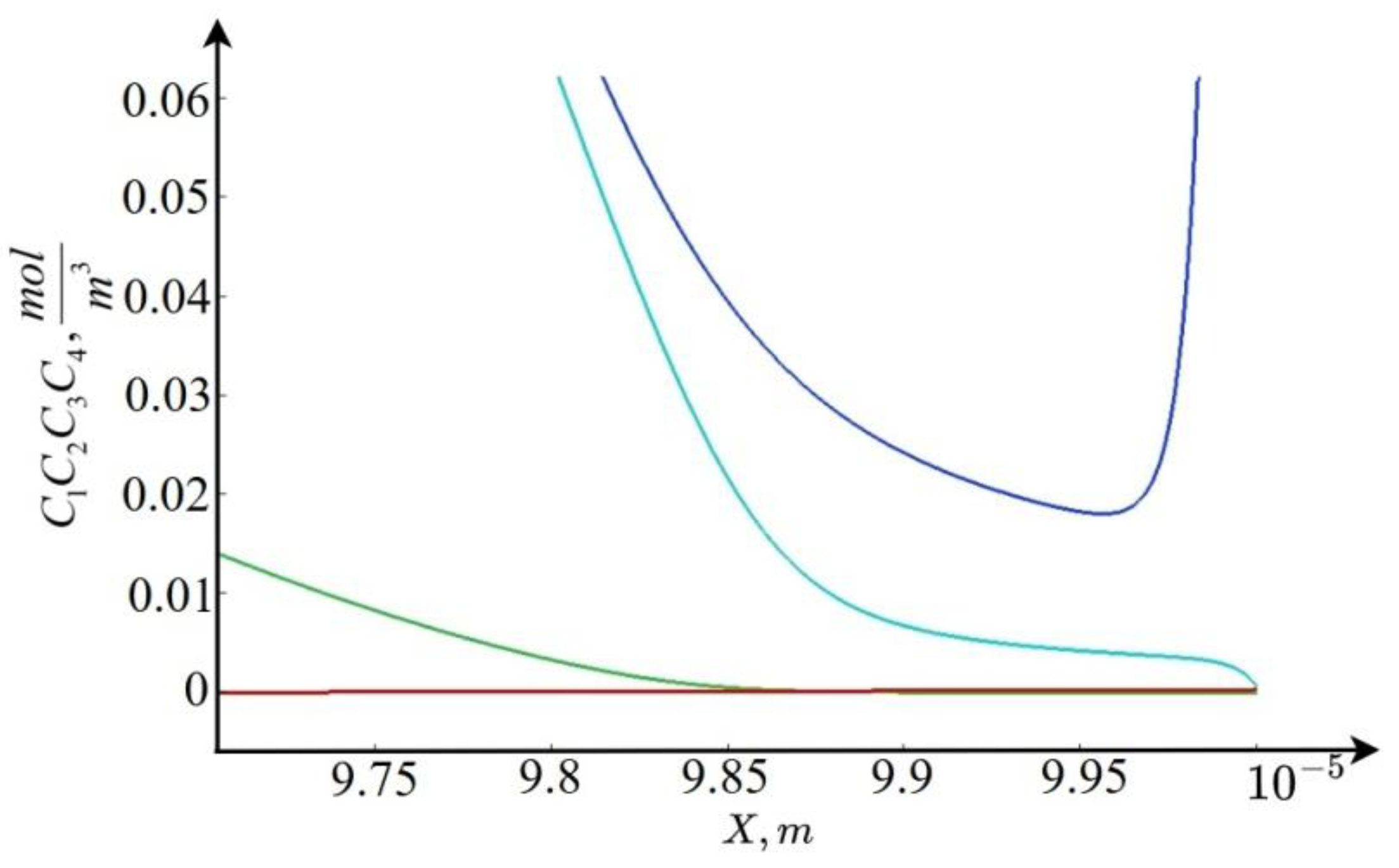
Figure 3. Graphs of concentrations in the extended space charge region: blue is the concentration of cations, light blue is the concentration of

O H^{-}

, green is the concentration of anions, red is the concentration of

H^{+}

ions.

Figure 3. Graphs of concentrations in the extended space charge region: blue is the concentration of cations, light blue is the concentration of

O H^{-}

, green is the concentration of anions, red is the concentration of

H^{+}

ions.

Using these relations, the original system of equations in the extended space charge region can be simplified:

ε \frac{d^{2} φ}{d x^{2}} = - (C_{1} - C_{4})

(25)

\frac{d C_{1}}{d x} = - C_{1} \frac{d φ}{d x} - j_{1}

(26)

\frac{d C_{4}}{d x} = C_{4} \frac{d φ}{d x} - j_{4}

(27)

ε D_{i} \frac{d j_{i}}{d x} = a (k_{w_{0}} + β (C_{1} - C_{4}))

(28)

An approximate solution to the system (25)-(28) depends on the relationship

k_{w_{0}}

and

β \sqrt{ε}

, which is determined by the value

C_{0}

. For small

C_{0}

, we have

\frac{k_{w_{0}}}{β \sqrt{ε}} > > 1

, and for large

C_{0}

, on the contrary

\frac{β \sqrt{ε}}{k_{w_{0}}} > > 1

, and for some

C_{0}

, we obtain

\frac{β \sqrt{ε}}{k_{w_{0}}} = О (1)

1) Let

\frac{k_{w_{0}}}{β \sqrt{ε}} > > 1

, then discarding the second term on the right-hand side of equation (28), we obtain the expression for the flows

j_{i} (x, ε) = j_{i} (x_{c}) + \frac{a k_{w_{0}}}{ε D_{i}} (x - x_{c})

From this formula it is clear that the effect of changing the equilibrium coefficient at

\frac{k_{w_{0}}}{β \sqrt{ε}} > > 1

in the extended region of space charge on the flows

j_{i} (x, ε)

and, accordingly, the distribution of the concentration and electric field strength is insignificant, and the flows themselves increase linearly (see Figure 4).

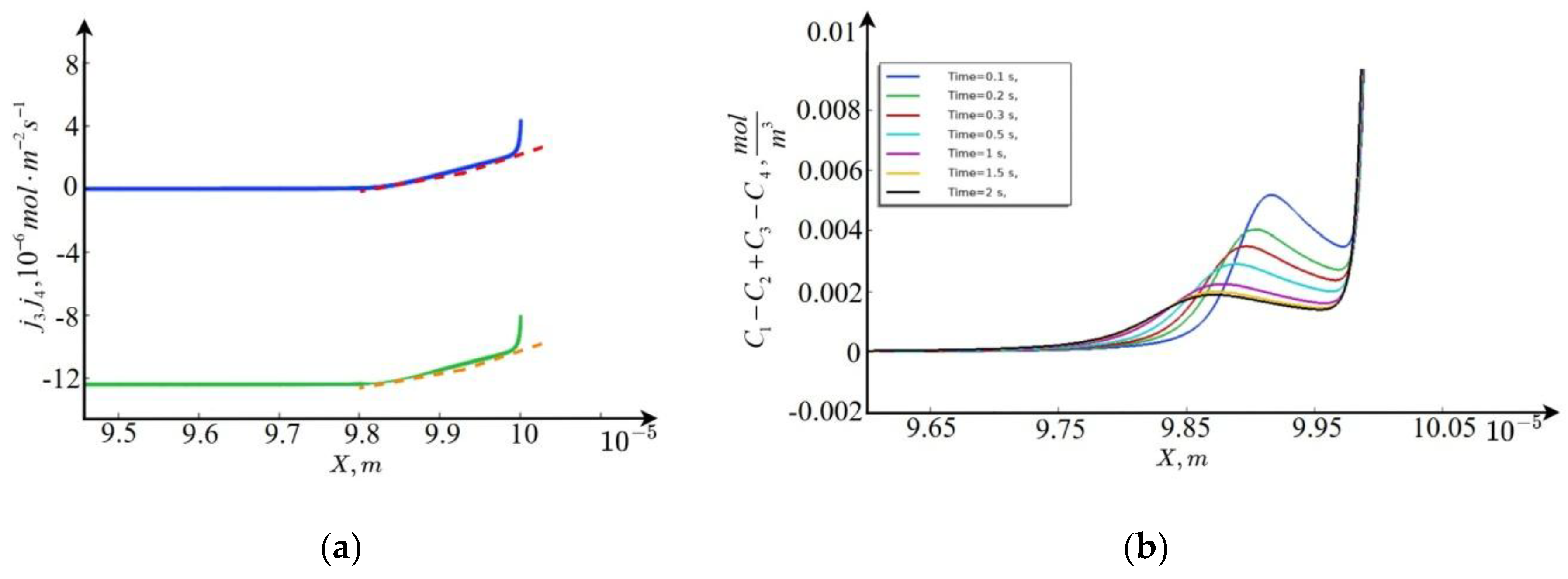
Figure 4. (a) – graphs of

j_{3}

(blue line) and

j_{4}

(green line) calculated numerically (solid line) and analytically (dashed line), (b) – graphs of space charge for different t.

Figure 4. (a) – graphs of

j_{3}

(blue line) and

j_{4}

(green line) calculated numerically (solid line) and analytically (dashed line), (b) – graphs of space charge for different t.

For an analytical solution, we derive an equation for the electric field strength independent of the remaining unknowns.

The system of equations has a first integral

C_{1} + C_{4} = \frac{ε}{2} Е^{2} - \frac{a k_{w_{0}}}{2 ε D_{4}} {(x - x_{c})}^{2} - (j_{1} + j_{4} (x_{c})) (x - x_{c}) + γ

From equations (26), (27) we have the relation

j_{1} - j_{4} = (C_{1} + C_{4}) Е - \frac{d (C_{1} - C_{4})}{d x}

Substituting into which the first integral and the value

j_{4}

, we obtain the equation:

ε \frac{d^{2} Е}{d x^{2}} = (\frac{ε}{2} Е^{2} - \frac{a k_{w_{0}}}{2 ε D_{4}} {(x - x_{c})}^{2} - (j_{1} + j_{4} (x_{c})) (x - x_{c}) + γ) Е + \frac{a k_{w_{0}}}{ε D_{4}} (x - x_{c}) - j_{1} + j_{4} (x_{c})

Using asymptotic estimates, it can be shown that the left-hand side of the equation in the extended region of the space charge is small compared to the remaining terms of the equation. As a result, to find the electric field strength, we obtain the equation

\frac{ε}{2} Е^{3} - (\frac{a k_{w_{0}}}{2 ε D_{4}} {(x - x_{c})}^{2} + (j_{1} + j_{4} (x_{c})) (x - x_{c}) - γ) Е + \frac{a k_{w_{0}}}{ε D_{4}} (x - x_{c}) - j_{1} + j_{4} (x_{c}) = 0

which has one isolated positive solution, using which, we find the remaining functions from the solution of linear equations (26), (27).

2) Let

\frac{β \sqrt{ε}}{k_{w_{0}}} > > 1

Using equations (25) and (28) we obtain the relationship

j_{4}

and

ϕ

, namely, from one equation we express

C_{1} - C_{4}

and substitute into the other, and integrating which, we obtain

D_{4} j_{4} = - a β \frac{d ϕ}{d x} + γ_{1}

, where

γ_{1}

is the integration constant. Let us write this equation using the electric field

E = - \frac{d ϕ}{d x}

strength as:

ε D_{i} \frac{d j_{i}}{d x} = a (k_{w_{0}} + β (C_{1} - C_{4}))

(29)

where we can see the linear dependence of the

H^{+}

and

O H^{-}

flows on the electric field strength

E

in the extended space charge region.

Substitute

j_{4}

into equation (27) and after a series of transformations we obtain the first integral of the system

C_{1} + C_{4} = \frac{ε}{2} {(\frac{d ϕ}{d x})}^{2} + \frac{a β}{D_{4}} ϕ - (\frac{γ_{1}}{D_{4}} + j_{1}) x + γ_{2}

, where

γ_{2}

is the integration constant.

Using the first equation and the first integral we obtain an equation for

ϕ

that does not contain other unknown functions:

- ε \frac{d^{3} ϕ}{d x^{3}} = - (\frac{ε}{2} {(\frac{d ϕ}{d x})}^{2} + \frac{a β}{D_{4}} ϕ - (\frac{γ_{1}}{D_{4}} + j_{1}) x + γ_{2}) \frac{d ϕ}{d x} - \frac{a β}{D_{4}} \frac{d ϕ}{d x} + \frac{γ_{1}}{D_{4}} - j_{1}

Asymptotic evaluation of the terms of this equation shows that the term on the left-hand side of the equation is small compared to the remaining terms, so the equation can be used to calculate the potential:

(\frac{ε}{2} {(\frac{d ϕ}{d x})}^{2} + \frac{a β}{D_{4}} ϕ - (\frac{γ_{1}}{D_{4}} + j_{1}) x + γ_{2} + \frac{a β}{D_{4}}) \frac{d ϕ}{d x} - \frac{γ_{1}}{D_{4}} + j_{1} = 0

This equation is solved analytically by introducing the parameter [27]. After determining

ϕ

, the remaining unknown functions are also found analytically from the solution of the linear equations (26), (27).

5.3. Analytical Solution in a Quasi-Equilibrium SCR on the Segment $(x_{q}; 1]$

In the case where the equilibrium coefficient does not depend on the space charge in this region, the flows of hydrogen and hydroxyl ions increase linearly, i.e. dissociation occurs with the maximum possible constant rate. However, when it depends on the space charge, the flows of hydrogen and hydroxyl ions increase with an exponential rate, i.e. the second Wien effect comes into play and the rate of dissociation of water molecules increases by many orders of magnitude.

From the analysis of the numerical solution it follows that this region is a quasi-equilibrium region of space charge,

x_{q} (ε) \to 0, ε \to 0 +

and

C_{1} (х, ε)

, exponentially increases

C_{2} (х, ε) \approx 0

C_{3} (х, ε)

, has a local maximum,

C_{4} (х, ε)

exponentially decreases to zero,

С_{3} < < C_{1},

С_{4} < < C_{1}

C_{4} C_{3} < < C_{1}

. In addition,

j_{3} (х, ε)

and

j_{4} (х, ε)

increase with the rate of the exponential.

Taking these assumptions into account, we obtain the following system of equations:

\frac{d C_{1}}{d x} = - C_{1} \frac{d ϕ}{d x},

(30)

\frac{d C_{3}}{d x} = - C_{3} \frac{d ϕ}{d x} - j_{3},

(31)

ε \frac{d j_{3}}{d x} = a (k_{w_{0}} + b_{0} С_{1}),

(32)

ε \frac{d^{2} ϕ}{d x^{2}} = - С_{1} .

(33)

Integrating (30) from point

x_{q}

to arbitrary point

x

, we obtain

С_{1} = С_{1 q} e^{- h_{0} \frac{ϕ - ϕ_{0}}{h_{0}}} = С_{1 q} e^{- h_{0} \frac{d ϕ}{d x}} = С_{1 q} e^{h_{0} E}

where

h_{0} = x - x_{q}

, and, accordingly, we have:

k_{w} (ρ) \approx k_{w_{0}} + λ С_{1 x_{0}} e^{h_{0} E} .

(34)

Thus, in a quasi-equilibrium SCR, the equilibrium coefficient exponentially depends on the electric field strength

E

It is easy to verify that the system of equations (30) – (33) has an analytical solution:

E (x, ε) = \frac{1}{\sqrt{ε}} \frac{b - b γ e^{b \frac{x - 1}{\sqrt{ε}}}}{γ e^{b \frac{x - 1}{\sqrt{ε}}} + 1}

С_{1} (х, ε) = 2 b^{2} γ^{2} \frac{e^{2 b \frac{x - 1}{\sqrt{ε}}}}{{(γ e^{b \frac{x - 1}{\sqrt{ε}}} + 1)}^{2}}

j_{3} = \frac{a}{ε} k_{w_{0}} x + \frac{b_{0}}{\sqrt{ε}} 2 b \ln | γ e^{\frac{b}{\sqrt{ε}} (x - 1)} + 1 | + \frac{b_{0}}{\sqrt{ε}} 2 b \frac{1}{γ e^{\frac{b}{\sqrt{ε}} (x - 1)} + 1}

From this solution it follows that the thickness of the quasi-equilibrium region is of the order of

O (\sqrt{ε} \ln ε)

, i.e. the same as the width of the recombination region. This confirms the conclusions obtained using the similarity theory in Section 2.2.

6. Conclusion

A mathematical model of stationary transfer of a binary electrolyte in electromembrane systems is constructed taking into account the dissociation/recombination reaction and changes in the equilibrium coefficient. A similarity theory of the transfer process in the diffusion layer of a cation-exchange membrane has been developed. Using trivial similarity criteria, it has been shown that the size of the recombination region is of the same order of magnitude as the quasi-equilibrium region of the space charge. A non-trivial similarity criterion has been found and the contribution of the dissociation/recombination reaction of water molecules to the transfer of salt ions in the diffusion layer has been clarified. It has been shown that, assuming that the thickness of the diffusion layer remains constant, the effect of the dissociation/recombination reaction of water molecules decreases with increasing initial concentration of the solution and, conversely, increases with decreasing initial concentration at a quadratic rate. The similarity theory constructed above is of great importance for engineering calculations and for scaling experimental results. With increasing initial concentration of the solution, the value of the small parameter entering singularly decreases and reaches values of the order of 10^-12 or less, which leads to computational difficulties that do not allow an exhaustive analysis of the effect of changes in the equilibrium constant on the transport of salt ions. In this regard, an analytical solution to the problem has been constructed, based on the division of the solution was divided into a number of subregions (electroneutrality regions, extended space charge region, quasi-equilibrium region, recombination region, intermediate layer), in each of which the problem was solved in its own way, and then these solutions were merged. The analytical solution was verified by comparison with the numerical solution. The advantage of the obtained analytical solution is the possibility of an exhaustive analysis of the effect of the dissociation/recombination reaction of water molecules on the transfer of salt ions over a wide range of real changes in the concentration and composition of the electrolyte solution and other input parameters. For example, it was shown that the dependence of the equilibrium coefficient on the space charge leads to a linear dependence on the electric field strength in the extended space charge region and an exponential dependence on the electric field strength in the quasi-equilibrium space charge region. This is a non-trivial generalization of the assumption of an exponential dependence of the equilibrium coefficient on the electric field strength for bipolar ion-exchange membranes to the case of monopolar membranes. The boundary value problem solved in this work is a reference for constructing asymptotic solutions for other singularly perturbed boundary value problems of membrane electrochemistry.

Author Contributions

Conceptualization, N.C. and M.U.; methodology, E.K.; software, R.N.; validation, A.K., N.C. and M.U.; formal analysis, E.K.; investigation, R.N.; resources, A.K.; data curation, N.C.; writing—original draft preparation, M.U.; writing—review and editing, E.K.; visualization, R.N.; supervision, M.U.; project administration, E.K.; funding acquisition, A.K., N.C. and M.U. All authors have read and agreed to the published version of the manuscript.

Funding

This research was funded by the Russian Science Foundation, research project No. 24-19-00648, https://rscf.ru/project/24-19-00648/. Open Access funding provided by the Open Access Publication Fund of the RheinMain University of Applied Sciences-00648, https://ror.org/0378gm372

Data Availability Statement

The data will be made available by the authors on request.

Conflicts of Interest

The authors declare no conflicts of interest.

References

Probstein, R.F. Physicochemical hydrodynamics: An introduction; John Wiley and Sons Inc.: New York, 1994; 416p. [Google Scholar]
Newman, J.; Thomas-Alyea, K. E. Electrochemical systems, John Wiley & Sons, Inc.: Hoboken, New Jersey, Canada, 2004; 672 p.
Kovalenko, S.; Kirillova, E.; Chekanov, V.; Uzdenova, A.; Urtenov, M. Analytical Solutions and Computer Modeling of a Boundary Value Problem for a Nonstationary System of Nernst–Planck–Poisson Equations in a Diffusion Layer. Mathematics 2024, 12, 4040. [Google Scholar] [CrossRef]
Kovalenko, A.V.; Nikonenko, V.V.; Chubyr, N.O., Urtenov, M.K. Mathematical modeling of electrodialysis of a dilute solution with accounting for water dissociation-recombination reactions. Desalination 2023, 550, 116398. [CrossRef]
Yaroshchuk, A. Non-stationary ion transport through charged membranes: A numerical solution. Journal of Membrane Science 2000, 167, 1–17. [Google Scholar]
Nikonenko, V.V.; Pismenskaya, N. D.; Belova, E. I.; Sistat, P.; Huguet, P.; Pourcelly, G. Intensive current transfer in membrane systems: Modelling, mechanisms and application in electrodialysis. Advances in Colloid and Interface Science 2010, 160, 101–123. [Google Scholar] [CrossRef]
Biesheuvel, P. M.; Bazant, M. Z. Nonlinear dynamics of capacitive charging and desalination by porous electrodes. Physical Review E 2010, 81, 031502. [Google Scholar] [CrossRef] [PubMed]
Kim, S. J.; Han, J. Self-assembled monolayers for electrokinetic phenomena in microfluidics. Lab on a Chip 2008, 8, 1163–1170. [Google Scholar]
Kornyshev, A.A. Double-layer in ionic liquids: Paradigm change? The Journal of Physical Chemistry B 2007, 111, 5545–5557. [Google Scholar] [CrossRef]
Bazant, M. Z.; Squires, T. M. Induced-charge electrokinetic phenomena: Theory and microfluidic applications. Physical Review Letters 2004, 92, 066101. [Google Scholar] [CrossRef]
Kumar M.; Parul. Methods for solving singular perturbation problems arising in science and engineering, Mathematical and Computer Modelling. 2011, 54, 556–575.
Shiromani, R.; Shanthi, V.; Ramos, H. Numerical Treatment of a Two-Parameter Singularly Perturbed Elliptic Problem with Discontinuous Convection and Source Terms. Differ Equ Dyn Syst 2025, 33, 303–331. [Google Scholar] [CrossRef]
Kumar, M.H.; Saini, S. Various Numerical Methods for Singularly Perturbed Boundary Value Problems. American Journal of Applied Mathematics and Statistics 2014, 2.3, 129–142. [Google Scholar] [CrossRef]
Illingworth, T.C.; Golosnoy, I.O. Numerical solutions of diffusion-controlled moving boundary problems which conserve solute. Journal of Computational Physics 2005, 209, 207–225. [Google Scholar] [CrossRef]
Martín, J.; Rodríguez-Mateos, F.; Company, R. Analytic solution of mixed problems for thegeneralized diffusion equation with delay. Mathematical and Computer Modelling 2004, 40, 361–369. [Google Scholar] [CrossRef]
Krol, J. J.; Wessling, M.; Strathmann, H. Concentration polarization with monopolar ion exchange membranes: Current-voltage curves and water dissociation. Journal of Membrane Science 1999, 162, 145–154. [Google Scholar] [CrossRef]
Rubinstein, I.; Zaltzman, B. Electro-osmotic slip of the second kind and instability in concentration polarization at electrodialysis membranes. Mathematical Modelling and Numerical Analysis 2000, 34, 263–281. [Google Scholar] [CrossRef]
Bazant, M. Z.; Thornton, K.; Ajdari, A. Diffuse-charge dynamics in electrochemical systems. Physical Review E 2004, 70(2), 021506. [Google Scholar] [CrossRef]
Zholkovskij, E. K.; Masliyah, J. H. Electrokinetic phenomena in concentrated suspensions: Theory and experiment. Advances in Colloid and Interface Science 2004, 112, 59–83. [Google Scholar]
Manzanares, J. A.; Murphy, W. D. Electrokinetic phenomena in porous membranes: From ion transport to energy conversion. Journal of Membrane Science 2003, 212, 1–15. [Google Scholar]
Nikonenko V., V.; Pis’menskaya N., D.; Volodina E., I. Rate of Generation of Ions H+ and OH− at the Ion-Exchange Membrane/Dilute Solution Interface as a Function of the Current Density. Russ J Electrochem 2005, 41, 1205. [Google Scholar] [CrossRef]
Bard, A.J.; Faulkner, L.R. Electrochemical Methods: Fundamentals and Applications. Wiley: N-Y, USA, 2000; 864 p.
Urtenov, M.K.; Kovalenko, A.V.; Sukhinov, A.I.; Chubyr, N.O.; Gudza, V.A. Model and numerical experiment for calculating the theoretical current-voltage characteristic in electro-membrane systems. IOP Conference Series: Materials Science and Engineering 2019, 680, 012030. [Google Scholar] [CrossRef]
Uzdenova, A.M.; Kovalenko, A.V.; Urtenov, M.K.; Nikonenko, V.V. Theoretical Analysis of the Effect of Ion Concentration in Solution Bulk and at Membrane Surface on the Mass Transfer at Overlimiting Currents. Russian Journal of Electrochemistry 2017, 53, 1254–1265. [Google Scholar] [CrossRef]
Vasil’eva, A.B.; Butuzov, V.F. Singularly Perturbed Equations in Critical Cases; Moscow University: Moscow, Russia, 1978; p. 106. [Google Scholar]
Gudza, V. A.; Chubyr, N. O.; Kirillova, E. V.; Urtenov M. Kh . Numerical and asymptotic study of non-stationary mass transport of binary salt ions in the diffusion layer near the cation exchange membrane at prelimiting currents. Appl. Math. Inf. Sci. 15, 4, 411–422.
Boyce, W. E.; DiPrima, R. C., Elementary Differential Equations and Boundary Value Problems, 8th Edition, Wiley, New York, 2004. 625 p.

Disclaimer/Publisher’s Note: The statements, opinions and data contained in all publications are solely those of the individual author(s) and contributor(s) and not of MDPI and/or the editor(s). MDPI and/or the editor(s) disclaim responsibility for any injury to people or property resulting from any ideas, methods, instructions or products referred to in the content.

© 2025 by the authors. Licensee MDPI, Basel, Switzerland. This article is an open access article distributed under the terms and conditions of the Creative Commons Attribution (CC BY) license (http://creativecommons.org/licenses/by/4.0/).

Copyright: This open access article is published under a Creative Commons CC BY 4.0 license, which permit the free download, distribution, and reuse, provided that the author and preprint are cited in any reuse.

Downloads

Views

Comments

Subscription

Notify me about updates to this article or when a peer-reviewed version is published.

MDPI Initiatives

Important Links

Choose an area of interest and we will send you notifications of new preprints at your preferred frequency.

Disclaimer

Investigation Of The Boundary Value Problem For An Extended System Of Stationary Nernst-planck-poisson Equations In The Diffusion Layer

Abstract

Keywords:

Subject:

1. Introduction

2. Mathematical Model of the Influence of the Dependence of the Dissociation Coefficient on the Space Charge Value on the Stationary Transport of Salt Ions in the Diffusion Layer

2.1. System of Equations

2.2. Boundary Conditions

3. Trivial and Non-Trivial Similarity Criteria

3.1. Characteristic Quantities and Transition to Dimensionless Form

3.2. Physical Meaning of Similarity Criteria

4. Analysis of Numerical Solution and Algorithm of Analytical Solution

5. Analytical Solution

5.1. Analytical Solution in the Recombination Region [ x r − δ 1 , x r + δ 1 )

5.2. Analytical Solution in the Extended RPR

5.3. Analytical Solution in a Quasi-Equilibrium SCR on the Segment ( x q ; 1 ]

6. Conclusion

Author Contributions

Funding

Data Availability Statement

Conflicts of Interest

References

MDPI Initiatives

Important Links

Subscribe

5.1. Analytical Solution in the Recombination Region $[x_{r} - δ_{1}, x_{r} + δ_{1})$

5.3. Analytical Solution in a Quasi-Equilibrium SCR on the Segment $(x_{q}; 1]$