
Submitted:
18 March 2025
Posted:
18 March 2025
You are already at the latest version
Abstract
Buckled Rings, also known as Pressurized Elastic Circles, were first studied by Maurice Lévy , and then by Halphen and Greenhill . These planar curves can be described as critical points for a variational problem, namely the integral of a quadratic polynomial in the geodesic curvature of a curve. Thus they are a generalization of elastic curves, and they are solitary wave solutions to a flow in the (three-dimensional) filament hierarchy. An example of such a curve is the Kiepert Trefoil, which has three leaves meeting at a central singular point. Such a variational problem can be considered for curves in other surfaces. In particular, a recent paper of I. Castro et al found many examples of such curves in the unit sphere. In this article, which is in part an extension of that paper, we consider a new family of such curves, having a discrete dihedral symmetry about a central singular point. That is, these are spherical analogues of the Kiepert curve. We determine such curves explicitly using the notion of a Killing field, which is a vector field along a curve which is the restriction of an isometry of the sphere. The curvature k of each such curve is given explicitly by an elliptic function. If the curve is centered at the south pole of the sphere and has minimum value ρ, then k−ρ is linear in the height above the pole.
Keywords:
buckled ring
; filament equation
; soliton
1. Introduction
The classical elastica or elastic curve is a curve which is critical for the total squared curvature , where k is the (geodesic) curvature of the curve in the plane or space , and is a Lagrange multiplier acting to constrain the length of the curve. This is essentially the model of an elastic rod in equilibrium proposed by Daniel Bernoulli in 1743 in a letter to Euler. Using his newly developed Calculus of Variations, Euler was able to find a good qualitative description of all planar elastic curves.
In 1884, Maurice Lévy [1] developed a model of an elastic circle under uniform normal pressure, which was relevant to consideration of the stability of boiler tubes and flues and of the buckling of steel plates of a ship. Such a curve, known as a buckled ring or pressurized elastic circle is the solution to the variational problem of the elastica with an additional constraint corresponding to the area enclosed. Such closed curves tend to have n-fold rotational symmetry. In recent years, they have been of interest to cell biologists (see e.g. [5,6]), and as solitary wave solutions to an integrable system known as the planar filament equation (see e.g. [7,8]). The curvature of a solution curve satisfies a first order differential equation of the form , where is a polynomial of degree 4. Thus such curves have curvature given by elliptic functions.
The notion of a buckled ring can be extended to curves living on surfaces. These curves are solutions to variational problems of the form where is a quadratic polynomial in k. We will consider the case where the surface is the unit sphere. The quadratic term corresponds to the elastic energy and the constant term corresponds to the length constraint. The linear term corresponds to the area constraint; this is a consequence of the Gauss-Bonnet formula relating the area enclosed by a curve to the geodesic curvature of the boundary curve. In the planar case, the linear term does not play such a role; the integral of k around a simple closed curve is always . Nevertheless, the same curvature functions arise in the spherical case as the planar case. Solution curves are solitary wave solutions to the spherical version of the filament equation.
A recent paper of I. Castro et al [4] found many examples of buckled rings on the unit sphere. In this article, we consider a family of solutions having discrete dihedral symmetry about a singular central point. We explicitly solve the equation for the curvature. The resulting elliptic functions are periodic with two parameters and q, corresponding to the minimum value and the maximum value q. For specified value of , we find the ’rationality’ condition for the curve to close up in the desired way. The key tool for this construction is the use of a Killing field J, a vector field along the curve which is the restriction of a rotation field on the sphere, a notion introduced in [9]. The existence of such a field is a consequence of the integrability of the Hamiltonian system underlying the geometry.
2. Materials and Methods
Our jumping-off place is the notion of a spherical curve whose curvature depends on distance to a great circle, as discussed by Castro et al [4]. Consider curves on the unit sphere in with coordinates , where , is latitude and is longitude. Assume a curve on the unit sphere has curvature k satisfying . Let . According to [4], page 26, is a critical curve for the functional
and k satisfies the differential equation
Integrating, we have
A vector field J along the curve is a Killing field if it is the restriction of an infinitesimal isometry. Such a vector field can be recognized as satisfying the condition that it preserves the length and curvature of the curve. The first condition is , where T is the unit tangent vector. The second condition is , where N is the unit normal and is the Gauss curvature of the sphere. (See [9], page 8, for the proof of this statement.)
If we define along , then
So J is a Killing field along . Assume J vanishes when (the south pole). This implies when . So and
Eliminating a gives
Then since and when , we have
So we can rewrite the formula for as
Define q by the formula:
Then Equation 5 becomes
We choose q to be the other real root of with ; so the real solution satisfies . The quadratic discriminant is . When this is so for this is negative. Now we can solve 7 using formula 259.00 in [10], with their notation (so in particular, a and b from the formula are different from a and b elsewhere in this article):
and plugging into the formula, we get
is the Jacobi Elliptic Cosine function with modulus m. The curvature is periodic with period and satisfies .
We can choose coordinates on the sphere such that J vanishes at the north and south poles. Then we have given by equation 2. The curve passes through the south pole with curvature each period t tangent to a meridian . In order for the curve to have the proper form, we need to equal , where n is the number of leaves.
3. Results
The z coordinate of a buckled ring is given explicitly in terms of the Jacobi elliptic cosine. The coordinate can not in general be given in closed form, but it can be found by one quadrature. Since Mathematica 14 has built in routines for Jacobi elliptic functions, we are able to determine the precise values of the parameters corresponding to closed curve solutions such as the one shown in Figure 1.
Numerical investigations establish the existence of three-leaf buckled spherical rings for a significant range of values of . These curves are the spherical counterparts of the Kiepert trefoil, a buckled ring in the plane. In the planar case, such buckled rings are all related by similarity. Of course, no such relation can exist on the sphere. Even allowing the curvature at the vertex to be slightly negative results in such a curve. Figure 2 shows some examples of buckled rings.
For a given choice of the minimum curvature of the buckled ring, we may find the precise values of the maximum curvature q corresponding to solutions with n leaves. The following Table 1 gives some representative examples of such parameters.
4. Discussion
Buckled rings can be thought of as being created from closed curves of fixed perimeter containing fixed area, which minimize bending energy while subject to uniform external pressure. When the pressure is very great the curves are known to buckle into curves with n-fold dihedral symmetry. The curves studied in this article may be thought of as limit curves of this process, in which the curves make self-contact at a central point. While these may not be physically achievable, the curves are nevertheless natural as mathematical limits. Indeed, curves with multiple self-crossings, which would require the curve passing through itself, are still solutions to the buckled ring equation. (Examples may be found in [3] and in [7], Fig. 9.) From the point of view of soliton theory, all closed curve solutions are of interest.
The goal of this research has been to establish the existence of a family of such limit curves in the case where the ambient space has positive curvature. A natural extension of this to the case of negative ambient curvature is an area for future research.
Funding
This research received no external funding.
Institutional Review Board Statement
Not applicable.
Informed Consent Statement
Not applicable.
Data Availability Statement
Not applicable.
Conflicts of Interest
The author declares no conflicts of interest.
Abbreviations
The following abbreviations are used in this manuscript:
| MDPI | Multidisciplinary Digital Publishing Institute |
References
- Lévy, M. Mémoire sur un nouveau cas intégrable du problème de l’élastique et l’une de ses applications. Journal de Mathematiques Pures et Appliquees série 1884, 10, 5–42. [Google Scholar]
- Halphen, G. Traité des fonctions elliptiques et de leurs applications; Deuxième partie, Chap. V; Gauthier-Villars et fils: Paris, France, 1888. [Google Scholar]
- Greenhill, A. The elastic curve under uniform normal pressure. Math. Ann. 1889, LII, 465–500. [Google Scholar] [CrossRef]
- Castro, I., Castro-Infantes, I., & Castro-Infantes, J. (2023). Spherical curves whose curvature depends on distance to a great circle. In New Trends in Geometric Analysis: Spanish Network of Geometric Analysis 2007-2021 (pp. 19-42). Cham: Springer Nature Switzerland. [CrossRef]
- W. Helfrich, Elastic Properties of Lipid Bilayers: Theory and Possible Experiments, Z. Naturforsch. 28c (1973) 693-703. [CrossRef]
- S. Svetina, B. Žekš, Membrane bending energy and shape determination of phospholipid vesicles and red blood cells, Eur. Biophysics J 17 (1989), 101-111. [CrossRef]
- Arreaga, G., Capovilla, R., Chryssomalakos, C. and Guven, J. Area-constrained planar elastica, Phys. Rev. E 65, 031801. [CrossRef]
- G. Bor, M. Levi, R. Perline, S. Tabachnikov, Tire track geometry and integrable curve evolution, arxiv: 1705.06314. [CrossRef]
- Langer, J.; Singer, D.A. The total squared curvature of closed curves. J. Differential Geometry 1984, 20, 1–22. [Google Scholar] [CrossRef]
- Byrd, P. and Friedman, M. Handbook of elliptic integrals for engineers and physicists, Springer-Verlag, Berlin-Göttingen-Heidelberg, 1954. [CrossRef]
Figure 1.
(a) buckled ring; (b)vertical projection of the buckled ring to
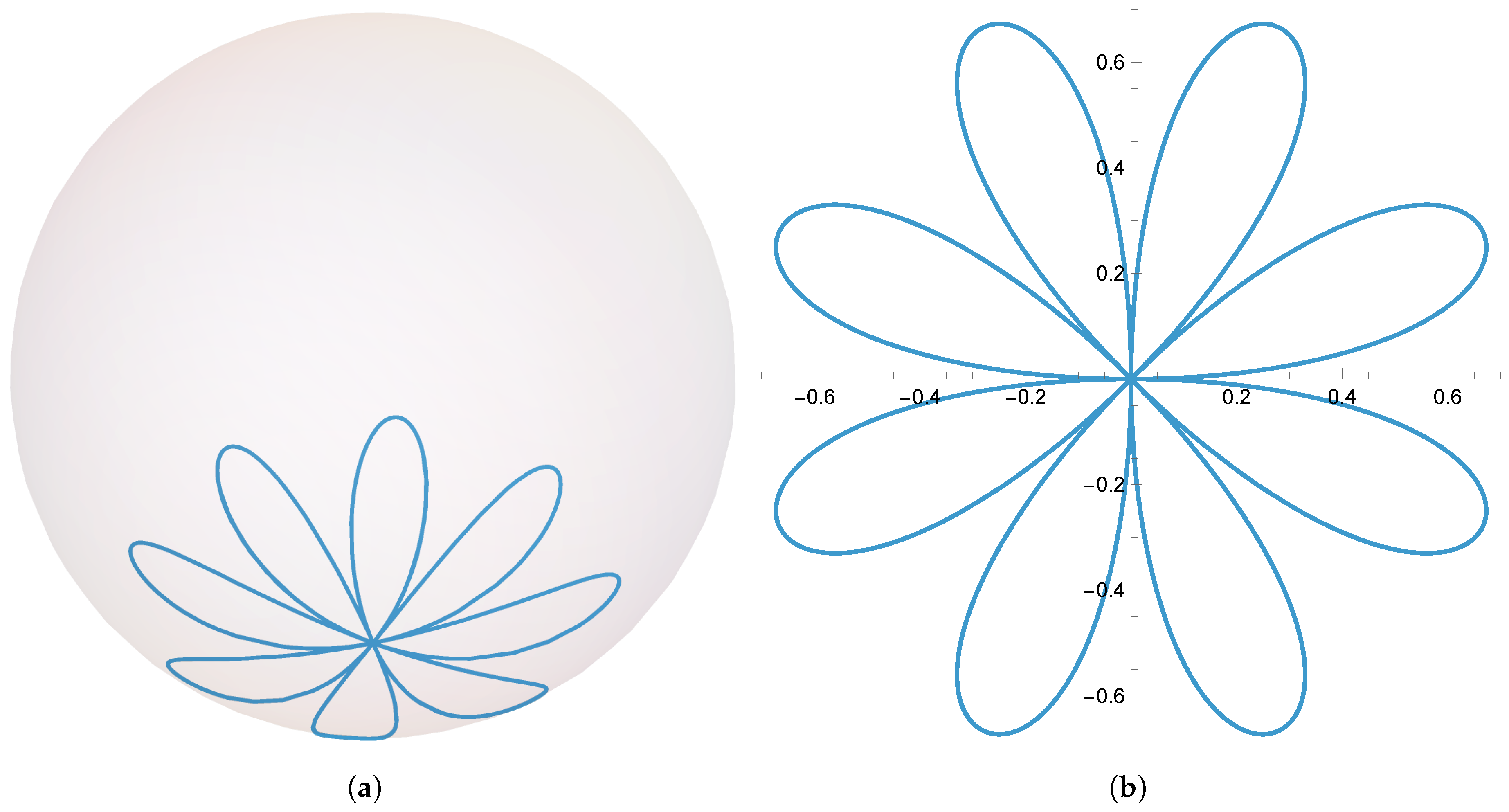
Figure 2.
(a) Three-leaf ring, . (b) Four-leaf ring, . (c) Three-leaf ring, . (d) - (f) Horizontal projections to the plane. (g)Three leaf ring with . (h). (i).
Figure 2.
(a) Three-leaf ring, . (b) Four-leaf ring, . (c) Three-leaf ring, . (d) - (f) Horizontal projections to the plane. (g)Three leaf ring with . (h). (i).
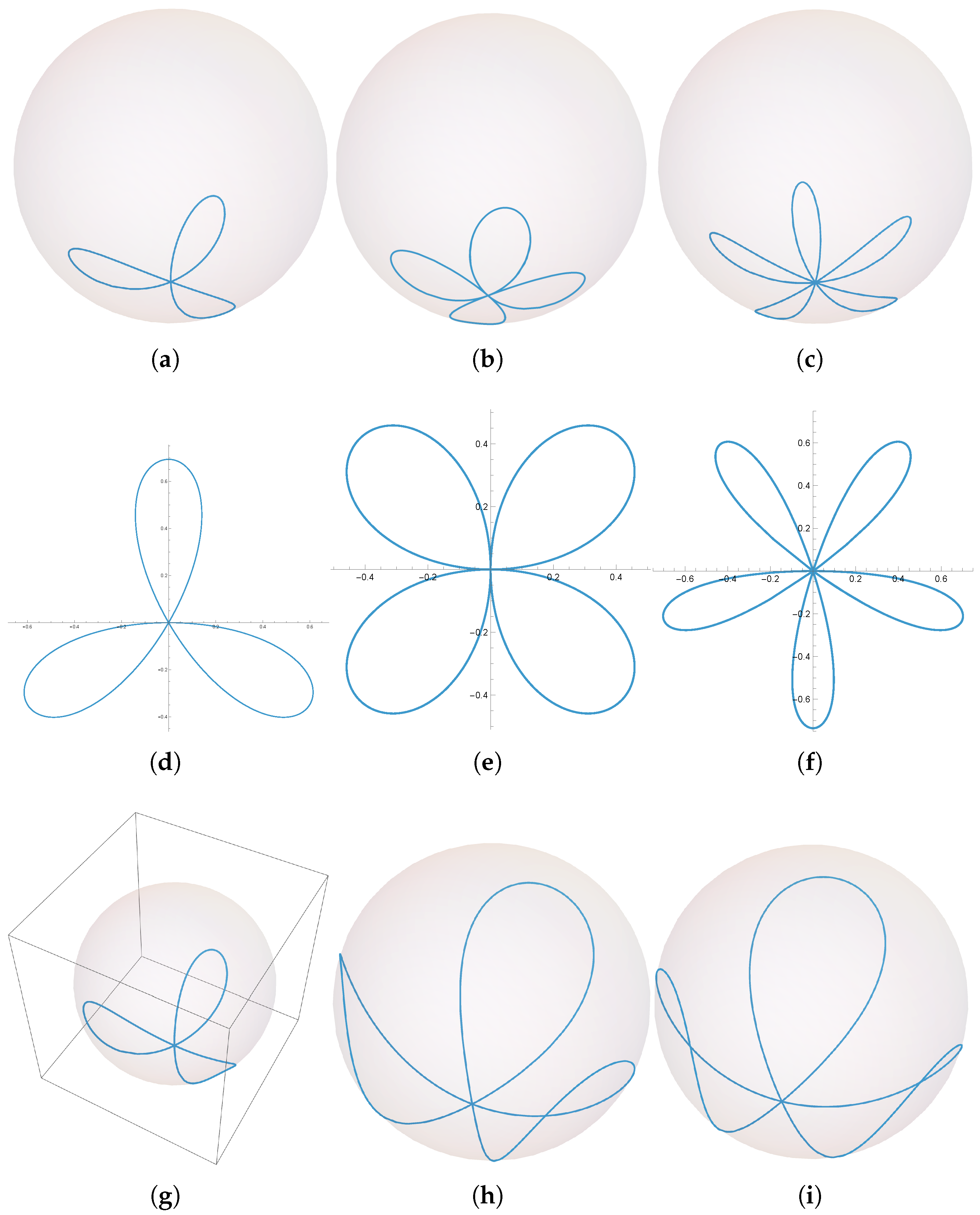

Table 1.
Examples of parameter values for closed curves.
| q | number of leaves | |
|---|---|---|
| 1.2455061500613556 | 1 | 4 |
| 1.4263123428252 | 1 | 3 |
| 1.5125430973168356 | 1 | 8 |
| 1.56315419238342057 | 1 | 5 |
| 1.29893522750021006565 | .5 | 3 |
| 1.4768833847622324 | .01 | 3 |
| 1.4846434986989393 | 0 | 3 |
Disclaimer/Publisher’s Note: The statements, opinions and data contained in all publications are solely those of the individual author(s) and contributor(s) and not of MDPI and/or the editor(s). MDPI and/or the editor(s) disclaim responsibility for any injury to people or property resulting from any ideas, methods, instructions or products referred to in the content. |
© 2025 by the authors. Licensee MDPI, Basel, Switzerland. This article is an open access article distributed under the terms and conditions of the Creative Commons Attribution (CC BY) license (http://creativecommons.org/licenses/by/4.0/).
Copyright: This open access article is published under a Creative Commons CC BY 4.0 license, which permit the free download, distribution, and reuse, provided that the author and preprint are cited in any reuse.


