

Submitted:
14 March 2025
Posted:
17 March 2025
You are already at the latest version
Abstract
In digital 3D reconstruction of shapes and surface reflectance of ancient paintings and drawings using Photometric Stereo (PS) techniques, normal integration is a key step. However, difficulties in locating light sources, non-Lambertian surfaces, and shadows make the results of this step inaccurate for such artworks. This paper presents a solution for PS to overcome this problem based on some enhancement of the normal integration process and the accurate measurement of Points of Interest (PoIs). The mutual positions of the LED lights, the camera sensor, and the acquisition plane in two custom-designed stands, are measured in laboratory as system calibration of the 3D acquisition workflow. After an introduction to the requirements and critical issues arising from the practical application of PS techniques to artworks, and a description of the newly developed PS solution, the measurement process is explained in detail. Finally, results are presented showing how normal maps and 3D meshes generated using the measured PoIs’ positions, and further minimized using image processing techniques, significantly limits the outliers and improves the visual fidelity of digitized artworks.
Keywords:
equipment measurement
; photometric stereo
; digital photogrammetry
; laser scanner
; painting 3D acquisition
; ancient drawing 3D acquisition
1. Introduction
Since 2010, our research team has developed a solution for the digitization, visualization of and interaction with ancient drawings and paintings addressed to various stakeholders engaged in paintings and ancient drawings’ knowledge, preservation, conservation and communication activities: museum visitors, art historians, restorers, professional operators and other figures. While the initial research was focused on the ancient drawings (mainly by Leonardo da Vinci) resulting in the successful application ISLe - InSight Leonardo [1], the approach was later extended to manuscripts as well as ancient paintings with the applications AnnunciatiOn App [2] and the recent GigaGuercino App. These outcomes follow a different trajectory from the usual answer given by the scientific community to the related issues, based on 2D outputs following two paths:
- Digital representations based on images with very high density of spatial content (i.e., the so-called gigapixel images). This solution is well illustrated by the Rijksmuseum’s 2019 gigantic Operation Night Watch project, which was able to reproduce Rembrandt’s painting with a resolution of 5 µm using 717 billion pixels [3].
- Images from Dome Photography (DP) that can be used in three ways: (1) visualization of the surface behavior of the artwork by interactive movement of a virtual light source over the enclosing hemisphere, i.e. the Reflectance Transformation Images (RTI) [4]; (2) 3D reconstruction of the object surface; (3) modelling of the specular highlights from the surface and hence realistic rendering.
These representations of paintings or drawings are generally accurate in resolution but limited to the simple reproduction of the apparent color and able to show the artwork just from a single, predefined point of view, missing the three dimensionality and reflectance properties. Paintings and drawings, instead, represent complex artistic creations, whose faithful knowledge though a copy implies the reproduction of the thickness and reflectance of brushstrokes, pens, and pencils (which provide insights into the techniques employed by painters), the subtle nuances of their surfaces, the presence of craquelures (valuable for determining the preservation state) and the optical properties of the papers and painting materials [5].
To meet these requirements, the solution developed by our team is 3D-based and rendered in real-time, allowing:
- the visualization of the artwork in a digital context that simulates the three-dimensional environment in which it is placed;
- the free exploration of the painting or drawing, allowing users to zoom in on details, to observe surface behaviors under changing lighting conditions and at different angles, and manipulate the artifact in real-time ‘as in your hands’ [6];
- the reproduction of the shape and the optical properties of the materials that make up the artwork, i.e., their total appearance [7].
In practice, the artwork is represented as a 3D model in a virtual space, and the optical behavior of its surface are modeled by tracing it back to phenomena belonging to three different scales: the microscopic scale, which can be summarized for artworks as their color (diffuse albedo), brilliance, and transparency/translucency; the mesoscale, which describes the roughness of the surface (what can be called 3D texture or topography); and finally the macroscopic scale, which can be described as the whole shape of the artefact [8].
Based on this modelling ranking, some software and techniques have been developed to return each scale correctly: nLights, a software based on Photometric Stereo (PS) [9], handles the mesostructure components; an analytically approximated Bidirectional Reflectance Distribution Function (BRDF) derived from the Cook-Torrance physical model and implemented via a shader allows to reproduce the microstructure [10,11]; and the SHAFT (SAT & HUE Adaptive Fine Tuning) program enable a faithful replica of the color [12]. Finally, macrostructure has been obtained from time to time using different techniques. In some cases, it was assimilated to a simple plane [13]; in others, a PS-based solution was used, exploiting computer graphics techniques to correct outliers [14]; and for the paintings, photogrammetric techniques were used as an efficient solution, as literature confirms [15].
Recently, we planned to merge all these solutions to have all-inclusive software, allowing a workflow, simple, accessible and economically viable for institutions of varying sizes and resources, accurate and to be used not only by expert researchers, but also by professionals of the Cultural Heritage (CH) sector for mass digitization operations of artworks [16]. A main goal of the new hardware/software system, with the aim to minimize the complexity of the process and the negatives effects of prolonged exposure of the artwork to the light, is the removal of double data collection techniques to reproduce surfaces and their optical behavior: photogrammetry techniques for the shape, and PS to extract optical reflectance properties [17]. Despite the well-known limitations of the PS techniques in shape reproduction, we based the whole process on these methods for their superior ability to accurately reproduce surface reflections. Custom-developed software and independently designed and manufactured repro stands [18] allows accurate results and a quick process from acquisition to visualization (Figure 1).
This paper delves into the solution developed for 3D reconstruction using PS techniques only, explaining problems and fixes, mainly focusing on the solution of the critical issues in the quantitative determination of surface normals. The assumption that the whole object is lit from the same illumination angle with the same illumination intensity across the entire field of view and the correct localization of the light sources, is a requirement rarely reached for a mismatch between the lighting model and real-world experimental conditions. When the surface normals are integrated, these inconsistencies result in incorrect surface normal estimations, where the shape of a plane becomes a so-called “potato-chip” shape [19,20,21]. In practice, as literature shows [22], calibrated PS with n ≥ 3 images is a well posed problem without resorting to integrability, but an error in the evaluation of the intensity of one light source is enough to cause a bias [23], and outliers may appear in shadow regions, thus providing normal fields that can be highly nonintegrable. To remove dependence on this far light assumption various techniques were developed but, in our opinion, not accurate enough for the art conservation where an accurate quantitative determination of surface’s normals is crucial.
The proposed solution is based on an accurate localization of the lights position through their measurement, and in some other enhancement to delete the residuals outliers. This solution has its rationale in the design of the hardware/software system that allows a single acquisition condition (artifacts larger than the framed field are reproduced by stitching multiple images), and hardware that keeps geometries and dimensions constant. Determining the mutual position of components can be considered a system calibration operation and can be done only once. In the following, the entire PS process is illustrated, as well as the refinements to eliminate noise due to non-Lambertian surfaces, shadows, approximate evaluation of light intensity, and its attenuation. Mainly the measurement process of the two different repro stands designed for capturing drawings and paintings (positioned horizontally and vertically) is presented.
The paper is organized in five main sections. After the Introduction, Section 2 begins with a state-of-the-art review of relevant techniques in PS, followed by the description of the PS software developed. Specifications and features of the developed stands conclude the paragraph. In Section 3 the metrological context is introduced, and it is illustrated the measurement approach for the ‘as built’ stands. Section 4 presents the results and Section 5 sums up the key points and findings of the research and examines possible future works.
2. The Photometric Stereo Framework
2.1. State of the Art
Originally introduced by Woodham [9] in the context of computer-based image interpretation, PS is a well-known computer vision approach frequently used to recover surface shape from image intensity. According to the principle that the intensity of the reflected light depends on the angle of incidence of the light on the surface, the technique estimates the surface orientation at any point of the object’s surface as a normal vector. The original formulation assumed lights infinitely far away, the camera orthographic, and the object surface Lambertian and convex (i.e. no shadows or inter-reflections). With a perfect Lambertian surface and in the absence of noise, three intensity values from non-coplanar light sources are sufficient to solve for both normal direction and surface albedo. In practice, for noisy image data, better results are obtained by taking the median of results for many triplets of light sources [24]. Traditional approaches [25,26,27] extract geometry from surface normals using gradient fields and three out of four lighting directions, where surfaces appear more Lambertian [28,29,30].
From the original introduction of PS, several researchers have attempted to generalize the technique for more realistic cameras, surfaces, and lighting models [31]. Belhumeur et al. [32] found that with an orthographic camera model and uncalibrated lighting, the surface of the object could be uniquely determined to within a bas-relief ambiguity. Papadhimitri and Favaro et al. [33] later suggested that this ambiguity is resolved under the perspective camera model. New techniques have been introduced based on non-Lambertian reflectance models [34,35,36,37] or sophisticated statistical methods to automatically filter out non-Lambertian effects [38,39]. The ‘bounded regression’ method [40], and the least median of squares for the regression joint with Gaussian radial basis functions are used to handle effects such as specular highlights and shadows [41].
Although often overlooked, issues relating to illumination are almost always the most important aspect to be considered in designing PS solutions. A 1% uncertainty in the intensity estimation will produce a 0.5-3.5-degree deviation in the surface normal orientation calculation [42]. Assumptions about parallel light and orthogonal projection often cause global shape deformation [43,44]. This deviation varies with surface properties and object dimensions. Several researchers [45,46] investigated removing the far-light assumption to improve the accuracy of PS. Others [47] consider further non-isotropic illuminations. Another direction of research on PS is in the study of more realistic lighting models, to simplify the acquisition of data. E.g., methods have been developed to handle images acquired under nearby point light illumination [48], which finds a natural application in LED-based PS [49]. PS can be ill-posed when lighting is unknown (uncalibrated PS). The problem must be reformulated globally, and the integrability constraint must be imposed. But even then, a low-frequency ambiguity known as the generalized bas-relief ambiguity remains [32]: it is necessary to introduce additional priors, a problem for which various approaches have been proposed [43].
While PS can capture fine details even on non-collinear objects [50,51,52], a common objection to PS is that it is prone to a low-frequency bias that can distort the global geometry [53]. Such a bias usually results from a contradiction between the assumptions behind the image formation model and the actual experiments, e.g., assuming a directional light source instead of a nearby point source. From a practical point of view, it is easier to remove the low-frequency bias by coupling PS with another 3D reconstruction method, such as shape-from-silhouette [54], multi-view stereo [26], or depth sensing [55]. In such work, PS provides the fine-scale geometric details that are combined with the coarse geometry provided by the alternative technique. A complete review of the literature coupled with a clear illustration of the PS framework is in [56].
2.2. The Adopted PS Solution
The software solution developed for PS, is a customization of the MATLAB PSBox by Ying Xiong [57] designed to be coupled with the two custom stands built for the image capture phase. While the initial version of nLights was based on four intensity values, the most recent version accommodates 8 different light directions (N, S, E, W, at 45° and 15° relative to the acquisition plane), maintaining a fixed camera position perpendicular to the artwork’s surface. Redundant conditions are used to refine the results by progressively discarding the closest values. nLights produces as outcomes:
- albedo map;
- normal map;
- depth map, by integration of estimated normal vector field;
- reflection map generated as difference of the apparent color with the albedo;
- mesh with a resolution of a vertex for each pixel (i.e., 40 mm) exploiting the MATLAB functions surfaceMesh and meshgrid. In practice for each pixel is generated a vertex with coordinates x,y. The z depth is derived from the depth map and finally a Delaunay triangulation generates the mesh. Mesh spatial density parameters can be adjusted through quadric decimation.
PSBox implements PS through a defined sequence of steps based on two series of images captured under the same sequence of illumination: the first set of images is a picture of a sphere; the second the object to be digitized. The sequence is:
- Circle fitting from manually selected points on a chrome sphere image;
- Light direction determination using the chrome sphere image;
- Light strength estimation and lighting matrix refinement through nonlinear least squares optimization;
- PS computation to generate albedo and normal maps;
- Depth map reconstruction by integration of estimated normal vector field.
In detail, PSBox calculates light source directions by analyzing specular highlights on a chrome sphere under the same light conditions of the artwork to be replicated, assuming an orthographic camera model. The function requires three key inputs: an image I of a specular chrome sphere, circle parameters defined by a 3x1 vector containing the sphere’s center coordinates and radius, and a threshold value that identifies specular highlights (e.g., 250 for 8-bit images). The algorithm processes these inputs to output a unit vector (3x1) representing the light source direction. This approach to the estimation of the light direction is the major drawback of the software. The parallel and uniform condition is violated using commonly available light sources, because it is impossible to have a distant lighting setup that implicitly requires a large space for the whole system. Moreover, since the radiance from the source at the surface falls off in accordance with the inverse square law, a longer working distance will tend to cause the radiance to drop rapidly, correspondingly decreasing the signal/noise ratio of the whole system. Secondly the evaluation of the light position and direction using the sphere is usually inaccurate (2–3-degree errors are common). All these lacks determine the configuration for the representation of a flat surface resembling a “potato-chip”.
Light strength in PSBox is estimated by solving a nonlinear least squares problem from M images that are indexed by i, and each image has N pixels that are indexed by j. The intensity of j-th pixel in i-th image is therefore denoted as Iij. At j-th pixel, denote nj the surface normal, j the albedo, and bj = ρjnj the scaled normal. Since each of the M images comes from different lighting directions li, the rendering function considering directional light plus the ambient component α can be expressed as:
So that the estimation of the whole scene property is an optimization problem that can be solved with:
The PS technique is integrated in PSBox by grouping pixels with similar shadow patterns in different images, then solving a least squares system for each group to find scaled normal vectors and finally separating results into albedo (surface reflectivity) and unit normal vectors. The code handles shadows through the mask input with numerical stability when at least 3 valid measurements per pixel are found.
Normal integration from gradient fields exploits the Frankot and Chellappa method [58] based on Fourier transforms, to regularize (i.e., to enforce integrability of) the gradients in the frequency domain. PSBox presents then all the problems of this solution:
- lack of precision at the border of rectangular domains, if the boundaries are not constrained;
inaccuracies for very low frequencies although the photometric gradients give a good representation of the spatial frequencies in the surface, right up to the Nyquist frequency. Errors can result in ‘curl’ or ‘heave’ in the base-plane [59].
Moreover, in the PSBox pipeline, the surface normals are estimated at first and then integrated into a height map. This strategy is, however, suboptimal, since any error in the normal estimation step will propagate during the subsequent normal integration one.
To solve the problems in the PSBox implementation, the following improvements have been introduced:
- A.
-
A nearby light source model is used so they can be modeled as a distant point light (this is possible when the working distance of an illuminator to an object surface is more than five times the maximum dimension of the light emitting area) [60]. The light position and direction are found trough measurement of the mutual position of the camera, lights and acquisition plane. This geometric constraint provides a robust and deterministic approach, as the spatial relationships between points are predetermined by the physical setup rather than relying on potentially error-prone manual fitting operations. We evaluated the required accuracy of the measurement of the components’ mutual position through a series of tests aiming to evaluate the maximum error possible. At the end of the PS process the maximum errors need to be as follows:
- 1.
- pixel in the final normal map (maximum angular difference of 0.5° in the evaluation of the direction of the normal);
- 2.
- 1 mm in the mesh.
In practice, we measured the distance between a synthetic plane and a plane as obtained from the PS solution developed by virtually changing the position of LED lights. Figure 2 demonstrates that the maximum error allowed in the measurement is 5 mm.
- B.
- Frankot and Chellappa’s method for normal integration failures is corrected following a series of observations. As noted in [22] the accuracy of Frankot and Chellappa’s method ‘relies on a good input scale’ and a big improvement could be achieved exploiting solutions able to run non-periodic surfaces (“The fact that the solution [of Frankot and Chellappa] is constrained to be periodic leads to a systematic bias in the solution” [61]) and to manage non-rectangular domain. The latter condition is negligible in our case because paintings and drawings usually have a rectangular domain or - if not - can be easily inscribed into a rectangle anyway. We made an improvement for the other conditions exploiting the solution suggested by Simchony et al. [62] that consists in solving the discrete approximation of the Poisson equation using the discrete Fourier transform, instead of discretizing the solution of the Poisson.
- C.
- The most common solution for the problem of wrong representation of the surface at low frequencies is to replace the inaccurate low frequencies of the photometric normal by the more accurate low frequencies of a surface constructed from a few known heights measured with a laser scanner, or a probe, or a photogrammetric process [20,63]. We developed a different process, similar to that proposed by [21] allowing also to minimize problems caused by other factors: shadows, irregularity of light sources and their position, different brightness of each light source, lack of perfect parallelism of light beams. We use the distribution of light irradiance sampled from a flat reference surface. The non-uniformity of the radiance distribution is compensated using the reference images. In practice a flat surface is measured covering the whole light field and the normal field is calculated. Different normal values are qualified as systematic distortions and their value is subtracted to the normal field of the represented object. With this solution, there is no additional significant time cost required to solve the PS problem, as the procedure remains a linear problem. Finally, a surface deformation correction is applied by a 3 x 3 three-dimensional parabolic fitting algorithm, exploiting the MATLAB function fit minimizing the error at the least squares through all the points of the surface [64].
2.3. The Hardware Solutions
The hardware part of the solution consists of two distinct repro stands, each one optimized for different scenarios and artwork positions: a horizontal repro stand with a mobile acquisition plane for movable artworks and a vertical robotized one for automatic acquisition of paintings and drawings hanging from walls or not movable.
2.3.1. The Horizontal Stand
The horizontal repro stand is sized 1,470 x 1,470 x 1,992 mm and it features an acquisition plane of 700 x 880 mm. Its structure includes two main elements (Figure 3), each independently transportable and assembled:
- 3.
- a lower frame with a capture surface (Figure 4, left), consisting of a sliding base equipped with rails for translation along both the axes of the acquisition plane.
- 4.
- a vertical frame system (Figure 4, right), designed to house lights and camera, composed of four uprights made from square aluminum profiles, held in place by components manufactured through 3D rapid prototyping.
The support frames for the surface feature four ground contact points, whose height can be adjusted using screws with the aim of precise leveling the acquisition plan. The vertical frame consists of a profile system topped by a truncated pyramidal box element, inside which the camera is positioned on a constrained slide.
This pyramidal system is designed to stand on four inclined vertical uprights, which also provide housing for the 32 LED lights manufactured by Relio Labs [65]. These lights feature a 4000 K Correlated Color Temperature (CCT), and an illuminance of 40,000 lux at 0.25 m, not generate any potentially harmful Ultra-Violet (UV) or Infra-Red (IR) emissions and adopt a TIR (Total Internal Reflection) lens type mounted on the photoemitting diode with an emission angle of 25°. With this lens, the luminance drops to less than 50% of the maximum value.
2.3.2. The Vertical Stand
The vertical repro stand is sized 2,625 x 1,572 x 2,447 mm and consists of three elements (Figure 5):
- a lower frame (1,800 x 1,100 x 400 mm), consisting of a raisable base equipped with a rail for translation along the horizontal axis of the entire structure. The raisable base comprises a lifting frame that can be disassembled into individual arms (300 or 600 mm long) (Figure 6, left);
- a vertical frame system composed of four carbon fiber uprights held in place by two lightweight aluminum cross-braces (Figure 6, middle);
- a trapezoidal frame (850 x 850 x 1,200 mm) to which Relio2 LED illuminants and the mounting system for the camera are secured (Figure 6, right).
The lower frame is constructed from aluminum profiles, assembled through joints secured by bolt connections. Through an electric stepper motor, the lower frame hosts two linear actuators able to translate the upper structure horizontally. The upper vertical frame assembly is made of four carbon tubes placed vertically into their circular seats in both the top and bottom aluminum custom cross-braces. A darkening system consisting of a black jersey fabric cover, shaped around the trapezoidal frame, completes the stand (Figure 7).
3. The Measurement Methodology
3.1. Metrological Context and Approach
A key step of our workflow is the measurement of the relative positions among: the camera, considered as the central point of its sensor plane; the capture plane, where drawings and paintings are placed; the light sources, corresponding to the weighted centroids of the different groups of four LED lamps. This includes not only their 3D digital representation according to the measurement [66], but also the processing algorithm capable of transforming the dataset into calibrated coordinates that can be visualized and analyzed and the metrological characteristics of the instrument. Metrological aspects directly influence the ‘raw’ data produced by spatial measurement and their evaluation is then important because of its role in defining and optimizing the entire measurement process [67].
The term metrics quality [68], well qualified by an extensive literature (e.g., [69,70,71,72,73,74]), is used to quantify how much aspects related to a measurement deviate from a predefined dimension. Metrics quality is typically evaluated using quantities such as a priori knowledge of the 3D imaging device for surface measurement capability (calibration and characterization), uncertainty (i.e., the superposition of trueness or accuracy (the mean of the measurement) and precision of the measurement (i.e., the standard deviation of the measurement)), and, finally, the traceability of the measurement process (i.e., “A property of a measurement result whereby the result can be related to a reference through a documented unbroken chain of calibrations, each of which contributes to the measurement uncertainty” [75]), taking into account the object material and local surface features.
In detail, the measured coordinates produced by a 3D imaging system must then be accompanied by a quantitative statement of their uncertainty. Existing standards and geometric features drive this evaluation. Figure 8, after [76,77] summarizes the main factors that affect the uncertainty in a 3D imaging system.
In this context, according to the International Vocabulary of metrology – Basic and general concepts and associated terms (VIM), resolution is “the smallest change in a measured quantity that causes a noticeable change in the corresponding display”, i.e., for 3D imaging systems, the minimum geometric detail that the rangefinder is capable of capturing. Obviously, this value represents the maximum resolution allowed by the 3D sensor. It can be divided into two components: the axial resolution, along the optical axis of the device (usually specified as z), and the lateral resolution, on the xy plane [78].
For 3D sensors, accuracy needs then to be evaluated in both the axial and lateral directions. In general, the depth accuracy is the most important. In literature, setting the resolution level of the range camera is not yet extensively codified. Usually, this parameter is qualitatively adjusted to generate a 3D model that visually contains details of interest. This general visual rule is a geometric transposition of Nyquist’s sampling theorem, according to which an analog signal can be reconstructed exactly from its sampled version if the sampling frequency is at least double the signal’s variation frequency [79]. In the geometric case, it is therefore assumed that detail is correctly acquired with a sampling step of at least half the size of the minimum detail of interest. As [80] points out this criterion gives a “rule of thumb” for estimating a minimum geometric sampling step below which it is certain that the smaller geometric detail will be lost.
While accuracy is affected by systematic errors, precision is mostly affected by random errors, resulting in a certain degree of unpredictability of the measured value. In the case of laser-based devices, the main source is the laser speckle effect [81]. In the photogrammetric process, precision defines the statistical noise of an adjustment, i.e., it models the internal correctness of a system [82]. As the Structure-from-Motion (SfM) methods [83] used for camera localization and orientation provide only limited information about the internal quality of the Bundle Adjustment (BA) process [84] (i.e., only the final reprojection error), this can be improved starting from the orientation results obtained in the free-network approach, by adding constraints linked to a set of targets measured with more than five times higher uncertainty. After a similarity transformation, these 3D coordinates could be compared with those previously measured with laser scanners. Residuals and corresponding statistics can then be derived [73].
For an active 3D sensor, uncertainty estimation can be done by acquiring the range map of a target whose shape is known in advance, such as a plane, and evaluating the standard deviation of each 3D point with respect to the ideal shape [85]. Since a range map can easily be generated from millions of points, statistical significance is implicit. For modeling applications, the uncertainty of the range sensor should not exceed a fraction of the resolution step to avoid topological anomalies in the final mesh [86]. A good guideline is to avoid a resolution level smaller than the measurement uncertainty of the instrument.
For the photogrammetry, usually, the uncertainty assessment is performed by comparing the achieved results to a ground truth, which should theoretically be two or three times more accurate than the expected results. Although this general approach may be seen as reasonable, to achieve better metrological traceability a geometric artefact with known form and size is frequently used and its measurement is compared with another made with another instrument, e.g. a laser scanner.
In practice, in our case, the measurement process follows the workflow shown in Figure 9. The metrics quality was evaluated starting from a reduced version of the German guidelines DIN VDI/VDE 2634 [87] and the VDI/VDE 2617 6.1 [88]. After a calibration/characterization step, the measurement of the lights/camera/plane system was made through a photogrammetric process with a Hasselblad X2D-100C camera. This measurement was compared with a laser scanning capture with a Leica RTC360 Time-of-Flight (ToF) Terrestrial Laser Scanner (TLS) system to assess the metric quality of the 3D model. The inter-comparison of laser scanner data used as a reference with dense stereo generated 3D data is a well-consolidated approach. Several papers illustrate problems and solutions, methods and best practices [89,90]. As metric reference to scale the photogrammetry data from a Scantech iReal M3 laser scanner ensuring measurement results more than five times accurate than the expected results as per ISO 14253 [76] are used.
3.2. The Instruments Used for Measurements
3.2.1. Scantech iReal M3 Laser Scanner
The Scantech iReal M3 laser scanner is a 3D handheld system that uses triangulation technology based on a dual infrared laser light source, one of which is a Vertical Cavity Surface Emitting Laser (VCSEL). At its core, the handheld scanner projects seven parallel infrared laser beams onto the scanned object whose reflected beam is analyzed and localized by two sets of calibrated industrial cameras. Operatively, the handheld system works with a positioning mechanism based on retroreflective targets, similar to stickers, which can be easily applied to various surfaces and create a Positioning Model (PM). This PM serves to orient the scanner within 3D space and establishes a coordinate system for measurement reporting. From the PM, a second scan with VCSEL light reconstructs the surface. The two cameras simultaneously detect both retroreflective targets using invisible infrared backlight, which can improve marker recognition and adaptability to black materials, and VCSEL-projected laser lines. The corresponding spatial coordinates (X, Y, Z) of points on the object detected by the laser beams can be calculated based on the parallax of the image obtained from the cameras. Measuring uncertainty essentially depends on the size of the distance between emitted laser and sensor, the diffraction of the light source, and the speckle effect. Technical specifications are in Table 3.
3.2.2. Laser Scanner Leica RTC360 Tof TLS System
The Leica RTC360 TLS system for the measurement exploits the Wave Form Digitizer Technology (WFD). WFD combines the ToF technique (where is measured the round-trip flight time of a laser beam emitted by a light source relative to a point on the object to be measured) and the phase shift (where the distance is calculated based on the time interval between a start and stop pulse, which is digitized from the received signal) (Figure 10). Compared to a pure ToF measurement system, WFD technology enables better overall measurement performance thanks to rapid distance measurements, reduced laser spot size, increased measurement accuracy. The measurement uncertainty depends on the signal-to-noise ratio and the pulse rise time. Technical specifications are in Table 4.
3.2.3. Hasselblad X2D-100C Camera
The photogrammetric measurement of both repro stands was carried out using a Hasselblad X2D-100C camera, whose technical specifications are in Table 1 of Section 2.3.1. As lens system was used a Hasselblad XCD 38mm f/2.5 V lens, whose technical specifications are in Table 5.
3.3. Calibration and Characterization of Measurement Instruments
System calibration/characterization plays a key role in ensuring metrics quality (i.e., for calibrated devices, precision and uncertainty coincide), and the system measurement accuracy is largely dependent on the calibration accuracy. The instrument calibration/characterization was then the first step of our measurement process.
For the two laser scanners used (see paragraph 3.2.1 and 3.2.2), the calibration certification of the manufacturer was used as first reference, but then the instruments were characterized through a planar artifact. As demonstrated by Russo et al. [92], the 3D analysis of a reference plane allows for simultaneous estimation of uncertainty and accuracy. The best-fitting plane is used as an approximation of the actual position of the physical plane, while the point-to-point distance of each 3D point belonging to the range map can be measured and characterized. Since the plane is constructed as the best fit of the original data, the average distance is automatically zero, and therefore no absolute precision error can be evaluated. The standard deviation provides an estimate of the distribution of values around the ideal plane and allows for the evaluation of measurement uncertainty. Furthermore, even though the mean is zero, the chromatic map of the deviation between point and plane allows to identify any non-random pattern due to error accumulation in specific areas and any errors arising from systematic causes (precision).
For photogrammetry, the self-calibration process was used [93,94]. The solution of a self-calibrating BA leads to the estimation of all internal parameters and Additional Parameters (APs), beginning with a set of manually measured image correspondences (tie points). The overall network geometry, particularly the configuration of the camera stations, is critical to the accuracy of the process.
All measurements were done in an environmentally controlled laboratory with a temperature of 20 ° ± 0.1 °∆C and a relative humidity of ∼50%. During measurement activities, access to the laboratory was strictly controlled and limited to authorized personnel only, to ensure the reliability of the measurements (the floor was prevented against undesired movements). Before proceeding with the measurement operations careful attention to the operator’s manual guidelines, combined with extensive experimentation, was paid. A diffused and controlled ambient light (LED) provides an illumination without cast shadows.
3.3.1. Calibration and Characterization of the Scantech iReal M3 Laser Scanner
At first, the system was calibrated using a plate provided by the manufacturer in combination with the iReal 3D software (version r2023) that assists the user for the correct procedure. The scanner characterization was then performed through the acquisition of a reference test field consisting of a laminated glass panel (dimensions: 600 x 700 mm, thickness: 12 mm, planarity guaranteed within 10 µm across the entire surface) coated with a matte white PolyVinyl Chloride (PVC) film (Figure 11). The acquisition of the plane was performed maintaining a constant distance of 400 mm from the plane and a sampling resolution of 0.10 mm, i.e. accurate more than five times of the resolution of the photogrammetry. Results are in Table 6 and Figure 12.
3.3.2. Characterization of the Leica RTC360 ToF TLS System
The characterization of the Leica RTC360 ToF TLS system was carried out through the acquisition of a reference test field consisting of the laminated glass panel described in section 3.3.1. In this case, the acquisition was performed maintaining a constant distance of 790 mm from the plane and a sampling resolution as that of the photogrammetric measurement of the stands (0.40 mm). Results are in Table 7 and Figure 13, which show that the distribution of measured values is well within the expected threshold.
3.3.3. Camera Calibration
The geometric calibration of a camera is defined as the determination of deviations of the physical reality from a geometrically ideal imaging system based on the collinearity principle: the pinhole camera. The measurement of parameters for the acquisition system (see Section 3.2.3) was carried out following guidelines from experimental studies [95] through the self-calibration process using Colmap software (version 3.8) [96]. As camera model, the Brown’s formula including 10 parameters was used [97]:
- Focal length (f): expressed in pixels
- Principal point coordinates (Cx, Cy): defined as the coordinates of the intersection point of the optical axis with the sensor plane, expressed in pixels
- Affinity and non-orthogonality coefficients (b1, b2): expressed in pixels
- Radial distortion coefficients (k1, k2, k3): dimensionless
- Tangential distortion coefficients (p1, p2): dimensionless
3.4. Description of the Measurement Processes
The measurement process covered:
- The acquisition of a series of coded RAD targets using the Scantech iReal M3 3D laser scanner to provide a metric reference to scale the model in the photogrammetric process (Section 3.4.1);
- The acquisition of the stands by the Leica RTC360 ToF TLS system (section 3.4.2);
- The acquisition of the stands by photogrammetry (Section 3.4.3);
- The comparison of the photogrammetric data with the Leica RTC360 ToF TLS system data (Section 3.4.4).
The required measurement uncertainty of the mutual positions among the camera image sensor plane, the acquisition plane, and the light sources to address correctly the PS process is 2 mm (see Section 2.2), but we decided to define as goal the double of this value, i.e., 1 mm and a reference uncertainty of 0.1 mm.
3.4.1. Target Acquisition Through Scantech iReal M3 3D Laser Scanner
16 reference markers consisting of coded Ringed Automatically Detected (RAD) targets, each 5 mm in diameter, were placed across one plane positioned horizontally for the measurement of the horizontal stand and vertically for the vertical one (Figure 15). Both the arrangement and number of targets followed the scanner manufacturer’s recommendations. Specifically, the targets were positioned to maintain distances between 20 and 100 mm from each neighboring target. The measurement lateral resolution was 0.1 mm. The measurement process begins by creating the PM. During this phase, the scanner must acquire all the targets on the planar surface to achieve stable target array position. Once the PM is established, the VCSEL light is activated, and surface data collection is performed at a constant distance of approximately 400 mm over the plane, maintaining a perpendicular orientation to the planar surface, even if the measurement angle could be modified to allow non-perpendicular scanning without compromising the accuracy of the distances, since the reference PM was already defined [69]. The acquired data set was subsequently processed using the iReal 3D software (version r2023) and exported in .E57 format, also preserving the RGB chromatic information collected by the device allowing to check the target centroid position visually.
3.4.2. Stands Acquisition with Leica RTC360 ToF TLS System
A point cloud was captured with a single station, both for the horizontal and vertical stands maintaining a medium distance of 790 mm from the stands and a sampling resolution as that of the photogrammetric measurement of the stands (1 mm). This resolution was reached setting the instrument to the maximum level of lateral resolution, checking that the output distance between the points was the established (i.e., 1 mm).
3.4.3. Stands Acquisition with Photogrammetry
To perform the measurement on both repro stands the conventional automatic photogrammetric pipeline was followed: image acquisition, camera calibration (see paragraph 3.3.3), image orientation, and dense image matching [98] to extract dense cloud points. Taking in account the maximum uncertainty in the measurement required by the PS algorithm for the Points of Interest (PoI), the Ground Sample Distance (GSD) is 0.20 mm (i.e., using the Nyquist sample theorem 0.4 mm) corresponding to a distance camera-to-object of ≈1000 mm as in:
where:
- D is the distance in mm from the acquisition plane;
- Sw is the camera sensor width expressed in mm (equal to 43.8 mm for the Hasselblad X2D-100C);
- imW is the image width expressed in pixels (equal to 11,656 pixels for the Hasselblad X2D-100C output);
- Fr is the focal length of the adopted lens expressed in mm (equal to 38 mm for the Hasselblad XCD 38mm f/2.5 V lens).
A second camera network parameter that influence a lot the accuracy of the process is the distance/baseline ratio. As demonstrated by Guidi et al. [99] for SfM-based processes best results are achieved for a range of 4.7–6.2. We adopted a medium ratio of 5.5 to fill this requirement. The image acquisition does not used rigidly connected cameras on a stable structure, but all the images were captured using a tripod remotely controlling the camera through Hasselblad Phocus to avoid direct physical interaction and motion blur effects. All photos were shot with the same photographic parameter setup, i.e. focus fixed at infinity, aperture f16, shutter 1 sec, and ISO 400. The shots were stored in Hasselblad’s raw .FFF format and processed in the Hasselblad Phocus software environment to get 8-bit .TIFF format rendered images in the sRGB color space for later use in photogrammetric alignment. Unsharp mask and denoise filters were applied according to the manufacturer’s specifications for that combination of lens, camera, exposure, ISO, and aperture.
For the needs of the vertical repro stand only, all the positions of the PoI were measured considering two distinct configurations: without the assembled occlusion system and with the assembled occlusion system, to evaluate displacements due to its installation.
The photogrammetric measurement was performed through multi-image capture of both systems from different camera positions, acquired following a convergent camera network surrounding the stand structures and their reference planes (Figure 16). The number of captures is as follows:
- n. 132 for the horizontal acquisition stand;
- n. 133 for the vertical robotic stand without darkening occlusion;
- n. 102 for the vertical robotic stand with darkening occlusion.
Each point of the stands is visible from a minimum of 8 cameras (Figure 17) and a constant overlap of 60% between successive shots was maintained, with a maximum angular deviation not exceeding 20 degrees. This camera network configuration selected, characterized by convergent shots capable of closing the capture ring, ensures robustness in camera positioning and alignment compared to a parallel camera arrangement, as documented in various works published in scientific literature [100,101,102].
Image alignment was performed with the open-source Colmap using images downscaled by a factor of 4 (2 times by each side) and limiting the number of key points to 20,000.
As in [99] we used the tie points’ reprojection error for checking the quality of the calibration and orientation steps. The processing workflow includes the following steps:
- Running the alignment procedure on the full set of images captured;
- Checking the reprojection error on the resulting tie points. If below 0.5 pixels, stop here, otherwise proceed with the next step;
- Deleting about the 10% of the tie points providing the higher reprojection error;
- Rerunning the BA step on the cleaned set of tie points and go back to step 2.
Results of the camera’s orientation and calibration were then imported in the Agisoft Metashape Professional software [103] to scale the cameras positions through the 16 coded RAD targets present in the scenes. Finally, the dense point clouds were generated at Ultra High quality, meaning that the original images were processed at their full resolution without any preliminary downscaling.
3.4.4. Comparison of the Photogrammetric and TLS Data
The last step of the process concerns the comparison of the data captured by photogrammetry and laser scanner in the open-source software CloudCompare version 2.13.2) [104]. The photogrammetric models were aligned with the laser scanner point clouds using CloudCompare’s implementation of the Iterated Closest Point (ICP) algorithm [105,106]. After the subsampling of the photogrammetric point clouds to get models with the same GSD of the ToF TLS models (1 mm). Residual deviation of the 3D coordinates gathered with photogrammetry from the reference point cloud was statistically analyzed to calculate the Root Mean Square (RMS) error, mean error, and histogram error. We made sure that the orientation step was iterated until the mean value was less than 0.5 mm, for each dense cloud. This allowed us to confirm that the alignment process was performed correctly, influencing this way the random error estimation with a systematic factor.
4. Results
The following section presents the results concerning the measurements of the stands, the comparison between the photogrammetric and the laser scanner measurements, and the improvement in the performances of the nLights software exploiting measured localizations of the lights and algorithmic refinements described in Section 2.2.
4.1. As-Built Measurement of the Horizontal Repro Stand
4.1.1. Measurement Using Scantech iReal M3 Laser Scanner
The Scantech iReal M3 laser scanner was employed to measure the position of the spatial coordinates of the centroids the 16 coded RAD targets used to scale the photogrammetric dense point cloud. These coordinates were exported in .CSV format. In Table 9 are the positions of coded targets.
4.1.2. Measurement Using Leica RTC360 ToF TLS System
The Leica RTC360 ToF TLS system was employed to get a measurement to compare with the photogrammetric’s one. A scan was acquired using the Cyclone Register 360+ software (version 2024.0.2.r26474). Then, to facilitate further processing, the raw data was exported in the .E57 format. The data exceeding the stands shape were erased within CloudCompare. The TLS yielded a dataset made of 88,732,868 points which, after the cleaning process of the elements outside the stand, remained 10,294,639 points.
4.1.3. Measurement with Photogrammetry
The photogrammetric measurement was employed to get a dense point cloud of the stand, scaled through the 16 coded RAD targets measured with the Scantech iReal M3 laser scanner. Data exceeding the stand’s shape, were cleaned within CloudCompare. The results are in Table 10:
4.1.4. Comparison Between ToF TLS and Photogrammetry
4.1.5. Measurement of Points of Interest (PoIs) for the Horizontal Repro Stand
The coordinates of the Points of Interest (PoIs), representing the camera sensor plane, the capture plane, and the light sources were extracted as 3D coordinates from the dense cloud generated by Agisoft Metashape Professional (Figure 19), through vector graphic interpolation. These values were exported to AutoCAD version 2024 in .DXF interchange format to describe all the points in a new reference system and the sensor position along a straight directrix perpendicular to the acquisition plane and having its trace coinciding with origin of the Cartesian axis.
In AutoCAD, numerical tolerances were set to the fifth decimal place to avoid missing data. with the origin positioned at the center of the framed rectangle on the stand base (500 x 375 mm). The extracted and transformed coordinate values of PoI are in Table 12.
4.2. As-Built Measurement of the Robotic Vertical Repro Stand
4.2.1. Measurement Using Scantech iReal M3 Laser Scanner
The Scantech iReal M3 laser scanner was employed to measure the position of the spatial coordinates of the centroids the 16 coded RAD targets used to scale the photogrammetric dense point cloud. These coordinates were exported in .CSV format. In Table 13 are the positions of coded targets.
4.2.2. Measurement Using Leica RTC360 ToF TLS System
The Leica RTC360 ToF TLS system was employed to get a measurement to compare with the photogrammetric’s one. A scan was acquired using the Cyclone Register 360+ software (version 2024.0.2.r26474). Then, to facilitate further processing, the raw data was exported in the .E57 format. The data exceeding the stands shape were erased within CloudCompare. The TLS yielded a dataset made of 165,536,379 points which, after the cleaning process of the elements outside the stand, remained 11,378,129 points for the repro stand with darkening fabric occlusion and a dataset made of 166,253,743 points which, after the cleaning process of the elements outside the stand, remained 11,419,578 points for the repro stand without darkening fabric occlusion.
4.2.3. Measurement with Photogrammetry
4.2.4. Comparison Between ToF TLS and Photogrammetry
To compare the two datasets, the point cloud from photogrammetry were resampled to have an average image GSD of ~1 mm. The comparison between the point cloud obtained from the ToF TLS and the dense cloud obtained through photogrammetry (Figure 20 and Figure 21) produced the following results (Table 16 and Table 17):
4.2.5. Measurement of Points of Interest (PoIs) for the Vertical Repro Stand
The coordinates of the Points of Interest (PoIs), representing the camera sensor plane, the capture plane, and the light sources were extracted as 3D coordinates from the dense cloud generated by Agisoft Metashape Professional (Figure 22), through vector graphic interpolation. These values were exported to AutoCAD version 2024 in .DXF interchange format to describe all the points in a new reference system and the sensor position along a straight directrix perpendicular to the acquisition plane and having its trace coinciding with origin of the Cartesian axis. In AutoCAD, numerical tolerances were set to the fifth decimal place to avoid missing data, with the origin positioned at the center of the framed rectangle on the stand base (500 x 375 mm). The extracted and transformed coordinate values are in Table 18 and Table 19, while PoI variations after assembling the darkening fabric occlusion are in Table 20.
4.3. Results in the Performance Optimization of PS Techniques Adopted
The acquired measurements were integrated into the nLights software to generate albedo, specular, and normal maps. The comparation to approaches that determine light source directions based on reflections from a sphere the method developed produces more detailed results, as illustrated in Figure 23 and Figure 24. The real-time rendering of the XVIII Century drawing of Figure 1 shows a significant visual enhancement (Figure 25).
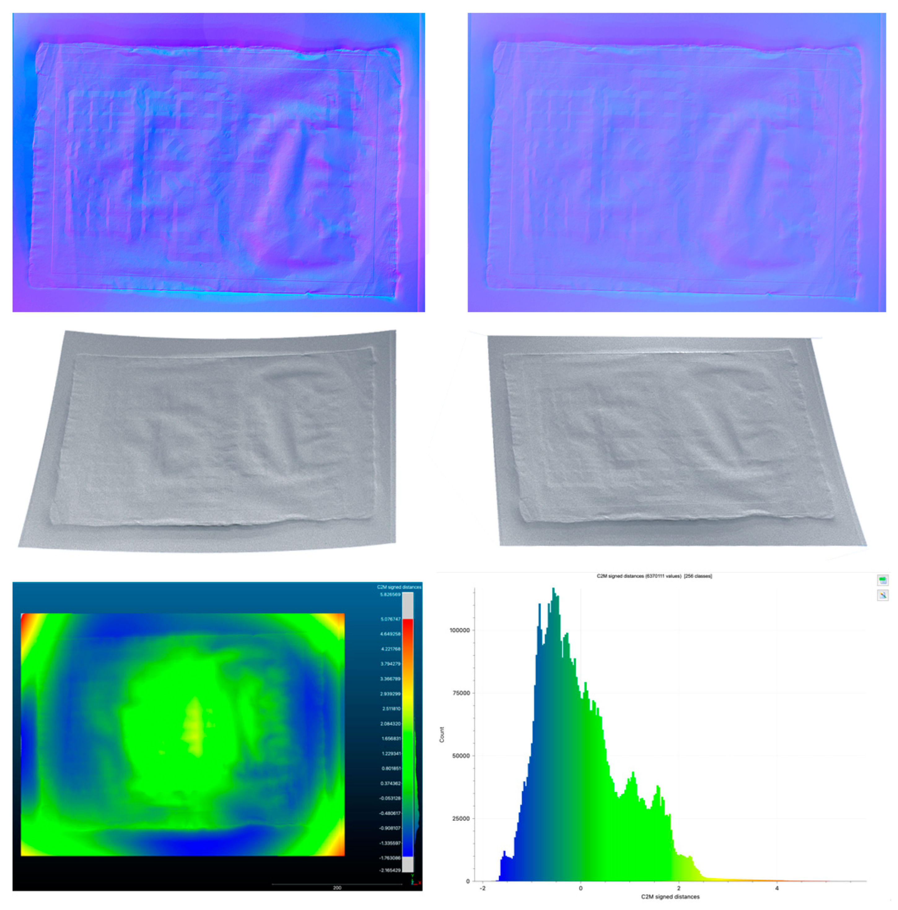
Finally, the results of the solution we developed to minimize problems caused by shadows, irregularity of light sources and their position, different brightness of each light source, and lack of perfect parallelism of light beams are presented. In Figure 26 are the normal maps and the meshes of a plane without and with correction. Normals’ colors are exaggerated for better visibility. The meshes are fitted against a reference plane. In Figure 27 are the results of the developed solution for the drawing in Figure 1 with both PoIs measured, and residuals of inaccurate low frequencies of the photometric normal minimized as illustrated in Section 2.2: normal maps with and without errors (top), meshes with and without outliers (middle), comparison between meshes with and without residuals (bottom). These results demonstrate strong improvements in the global shape representation.
5. Conclusions
This paper presents a solution for a PS technique able to overcome difficulties in normal integration, i.e. mainly issues in locating light sources, non-Lambertian surfaces, and shadows, to properly reconstruct in 3D the surfaces of artworks such as paintings and ancient drawings.
The solution, based on two key features (i.e., the use of image processing techniques to minimize residuals, and the measurement of the mutual positions of light sources, camera position and acquisition plane), proved to be successful in managing the mentioned criticalities.
Figure 27.
Results of the developed solution for the drawing of Figure 1, with and without outliers: normal maps with and without errors (top), meshes with and without outliers (middle), comparison between meshes with and without residuals (bottom).
Figure 27.
Results of the developed solution for the drawing of Figure 1, with and without outliers: normal maps with and without errors (top), meshes with and without outliers (middle), comparison between meshes with and without residuals (bottom).
In detail, the description of the complete processes of calibration, characterization and measurement of the two stands to find the PoIs, lets us substantiate the procedure and explain its efficiency.
In fact, despite its complexity, since the stands remain unchanged throughout their lifetime and are built with extremely low-deformation materials, once the entire measurement process is completed the end user is exempt from solving its problems by performing complex measurements, which are difficult to understand for most professional users working in the art world, for whom this solution is intended.
Future works may include the simplification of the measurement process to foster higher flexibility, allowing quick but accurate changes of parts in the hardware system (i.e., the lights, the camera and the stand).
Furthermore, more accurate techniques for the elimination of residuals for each specific stand will allow easy use of the whole technical solution for 3D acquisition and visualization of paintings and ancient drawings, which will enable greater involvement of professional operators working in the art reference field.
Author Contributions
Conceptualization, M.G. and S.G.; methodology, M.G.; software, M.G.; formal analysis, M.G. and S.G.; investigation, M.G., S.G. E.A.; data curation, E.A. and S.G.; writing—original draft preparation, E.A., M.G. and S.G.; writing—review and editing, E.A., M.G. and S.G.; visualization, E.A., and S.G.; supervision, M.G. All authors have read and agreed to the published version of the manuscript.
Funding
This research received no external funding.
Data Availability Statement
Upon a reasonable request from the corresponding author.
Acknowledgments
Authors would like to thank Giovanni Bacci for the support in the design and production of the stands’ prototypes and Andrea Ballabeni for the software development in all its stages.
Conflicts of Interest
The authors declare no conflicts of interest.
References
- Apollonio, F.I.; Bacci, G.; Ballabeni, A.; Foschi, R.; Gaiani, M.; Garagnani, S. InSight Leonardo – ISLE. In Leonardo, anatomia dei disegni; Marani, P., Ed.; Sistema Museale di Ateneo Università di Bologna: Bologna, Italia, 2019; pp. 31–45. [Google Scholar]
- Gaiani, M.; Garagnani, S.; Zannoni, M. Artworks at our fingertips: A solution starting from the digital replication experience of the Annunciation in San Giovanni Valdarno. Digital Applications in Archaeology and Cultural Heritage 2024, 33, 1–17. [Google Scholar] [CrossRef]
- Operation Night Watch at Rijks Museum. Available online: https://www.rijksmuseum.nl/en/stories/operation-night-watch/story/ultra-high-resolution-photo (accessed on 9 January 2025).
- Malzbender, T.; Gelb, D.; Wolters, H. Polynomial texture maps. In Proceeding of the 28th Annual Conference on Computer Graphics and Interactive Techniques (SIGGRAPH ‘01), ACM, New York, USA, 2001, pp. 519–528.
- Gaiani, M.; Apollonio, F.I.; Ballabeni, A.; Bacci, G.; Bozzola, M.; Foschi, R.; Garagnani, S.; Palermo, R. Vedere dentro i disegni. Un sistema per analizzare, conservare, comprendere, comunicare i disegni di Leonardo. In Leonardo a Vinci, Alle origini del genio, Barsanti, R. Ed.; Giunti Editore: Milano, 2019; pp. 207–240. [Google Scholar]
- Apollonio, F.I.; Gaiani, M.; Garagnani, S.; Martini, M.; Strehlke, C.B. Measurement and restitution of the Annunciation by Fra Angelico in San Giovanni Valdarno. Disegnare Idee Immagini 2023, 34, 32–47. [Google Scholar] [CrossRef]
- Eugène, C. Measurement of “total visual appearance”: A CIE challenge of soft metrology. In 12th IMEKO TC1 & TC7 Joint Symposium on Man, Science & Measurement proceedings, 2008, pp. 61–65. Available online: https://www.imeko.org/publications/tc7-2008/IMEKO-TC1-TC7-2008-006.pdf (accessed on 9 January 2025).
- Anderson, B.L. Visual perception of materials and surfaces. Current Biology 2011, 21, 978–983. [Google Scholar] [CrossRef] [PubMed]
- Woodham, R.J. Photometric method for determining surface orientation from multiple images. Opt. Eng. 1980, 19, 139–144. [Google Scholar] [CrossRef]
- Cook, R.L.; Torrance, K.E. A reflectance model for computer graphics. ACM Transactions on Graphics 1982, 1, 7–24. [Google Scholar] [CrossRef]
- Sole, A.; Farup, I.; Nussbaum, P.; Tominaga, S. Bidirectional reflectance measurement and reflection model fitting of complex materials using an image-based measurement setup. Journal of Imaging 2018, 4, 136. [Google Scholar] [CrossRef]
- Gaiani, M.; Ballabeni, A. SHAFT (SAT & HUE Adaptive Fine Tuning), a new automated solution for target-based color correction. In Colour and Colorimetry Multidisciplinay Contributions; Marchiafava,V.; Luzzatto, L., Eds.; Milan, Italy: Gruppo del Colore - Associazione Italiana Colore, 2018, XIVB, pp. 69–80.
- Gaiani, M.; Apollonio, F.I.; Clini, P. Innovative approach to the digital documentation and rendering of the total appearance of fine drawings and its validation on Leonardo’s Vitruvian Man. Journal of Cultural Heritage 2015, 16, 805–812. [Google Scholar] [CrossRef]
- Apollonio, F.I.; Foschi, R.; Gaiani, M.; Garagnani, S. How to Analyze, Preserve, and Communicate Leonardo’s Drawing? A Solution to Visualize in RTR Fine Art Graphics Established from “the Best Sense”. ACM J. Comput. Cult. Herit. 2021, 14, 1–30. [Google Scholar] [CrossRef]
- MacDonald, L.W.; Nocerino, E.; Robson, S.; Hess, M. 3D Reconstruction in an Illumination Dome. In Proceedings Electronic Visualisation and the Arts (EVA), London, UK, 9-13 July 2018, pp. 18–25.
- Apollonio, F.I.; Gaiani, M.; Garagnani, S. Visualization and Fruition of Cultural Heritage in the Knowledge-Intensive Society: New Paradigms of Interaction with Digital Replicas of Museum Objects, Drawings, and Manuscripts. In Handbook of Research on Implementing Digital Reality and Interactive Technologies to Achieve Society 5.0; Ugliotti, F.M., Osello, A., Eds.; IGI Global: Hershey, PA, USA, 2022, pp. 471–495.
- Karami, A.; Menna, F.; Remondino, F. Combining Photogrammetry and Photometric Stereo to Achieve Precise and Complete 3D Reconstruction. Sensors 2022, 22, 8172. [Google Scholar] [CrossRef]
- Bacci, G.; Bozzola, M.; Gaiani, M.; Garagnani, S. Novel Paradigms in the Cultural Heritage Digitization with Self and Custom-Built Equipment. Heritage 2023, 6, 6422–6450. [Google Scholar] [CrossRef]
- Huang, X.; Walton, M.; Bearman, G.; Cossairt, O. Near light correction for image relighting and 3D shape recovery. In Proceedings of Digital Heritage, Granada, Spain, 2015, 215-222.
- Macdonald, L.W. Representation of Cultural Objects by Image Sets with Directional Illumination. In Proceedings of the 5th Computational Color Imaging Workshop - CCIW, Saint Etienne, France, 24-26 March 2015, pp. 43–56.
- Sun, J.; Smith, M.; Smith, L.; Farooq, A. Sampling Light Field for Photometric Stereo. International Journal of Computer Theory and Engineering 2013, 5, 14–18. [Google Scholar] [CrossRef]
- Quéau, Y.; Durou, J.D.; Aujol, J.F. Normal Integration: A Survey. J Math Imaging Vis 2018, 60, 576–593. [Google Scholar] [CrossRef]
- Horovitz, I.; Kiryati, N. Depth from gradient fields and control points: Bias correction in photometric stereo. Image Vis. Comput. 2004, 22, 681–694. [Google Scholar] [CrossRef]
- MacDonald, L.W.; Robson, S. Polynomial texture mapping and 3D representation. In Proceedings of the ISPRS Comm. V Symposium Close Range Image Measurement Techniques, Newcastle, UK, 21-24 June 2010.
- Antensteiner, D.; Štolc, S.; Pock, T. A review of depth and normal fusion algorithms. Sensors 2018, 18, 431. [Google Scholar] [CrossRef]
- Li, M.; Zhou, Z.; Wu, Z.; Shi, B.; Diao, C.; Tan, P. Multi-View Photometric Stereo: A Robust Solution and Benchmark Dataset for Spatially Varying Isotropic Materials. IEEE Transactions on Image Processing 2020, 29, 4159–4173. [Google Scholar] [CrossRef]
- Rostami, M.; Michailovich, O.; Wang, Z. Gradient-based surface reconstruction using compressed sensing. In Proceedings of the 2012 19th IEEE International Conference on Image Processing (ICIP), Orlando, FL, USA, 30 September–3 October 2012; pp. 913–916.
- Solomon, F.; Ikeuchi, K. Extracting the shape and roughness of specular lobe objects using four light photometric stereo. IEEE Trans. Pattern Anal. Mach. Intell. 1996, 18, 449–454. [Google Scholar] [CrossRef]
- Barsky, S.; Petrou, M. The 4-source photometric stereo technique for three-dimensional surfaces in the presence of high-lights and shadows. IEEE Trans. Pattern Anal. Mach. Intell. 2003, 25, 1239–1252. [Google Scholar] [CrossRef]
- Cox, B.; Berns, R. Imaging artwork in a studio environment for computer graphics rendering. In Proceedings of SPIE-IS&T Measuring, Modeling, and Reproducing Material Appearance, San Francisco, California, USA, 2015.
- Ackermann, J.; Goesele, M. A survey of photometric stereo techniques. Foundations and Trends in Computer Graphics and Vision 2015, 9, 149–254. [Google Scholar] [CrossRef]
- Belhumeur, P.N.; Kriegman, D.J.; Yuille, A.L. The Bas-Relief Ambiguity. Int. J. Comput. Vision 1999, 35, 33–44. [Google Scholar] [CrossRef]
- Papadhimitri, T.; Favaro, P. A new perspective on uncalibrated photometric stereo. In Proceedings of the IEEE Computer Society Conference on Computer Vision and Pattern Recognition, Portland, OR, USA, 2013, pp. 1474–1481.
- Hertzmann, A.; Seitz, S. Shape and materials by example: A photo- metric stereo approach. In Proceedings of the IEEE Computer Society Conference on Computer Vision and Pattern Recognition, Madison, WI, USA, 2003.
- Alldrin, N.; Zickler, T.; Kriegman, D. Photometric stereo with non- parametric and spatially-varying reflectance. In Proceedings of the 26th IEEE Conference on Computer Vision and Pattern Recognition, Anchorage, AK, USA, 2008, pp. 1–8.
- Goldman, D.B.; Curless, B.; Hertzmann, A.; Seitz, S.M. Shape and spatially-varying BRDFs from photometric stereo. IEEE Transactions on Pattern Analysis and Machine Intelligence 2010, 32, 1060–1071. [Google Scholar] [CrossRef]
- Ren, J.; Jian, Z.; Wang, X.; Mingjun, R.; Zhu, L.; Jiang, X. Complex surface reconstruction based on fusion of surface normals and sparse depth measurement. IEEE Trans. Instrum. Meas. 2021, 70, 1–13. [Google Scholar] [CrossRef]
- Wu, L.; Ganesh, A.; Shi, B.; Matsushita, Y.; Wang, Y.; Ma, Y. Robust photometric stereo via low-rank matrix completion and recovery. In Proceedings of the 10th Asian Conference on computer Vision, Computer Vision – ACCV, Queenstown, New Zealand, November 2010; pp. 703–717. [Google Scholar]
- Ikehata, S.; Wipf, D.; Matsushita, Y.; Aizawa, K. Robust photometric stereo using sparse regression. In Proceedings of the IEEE Computer Society Conference on Computer Vision and Pattern Recognition, Providence, Ri, USA; 2012; pp. 318–325. [Google Scholar]
- MacDonald, L.W. Colour and directionality in surface reflectance. In Proceedings of the Conf. on Artificial Intelligence and the Simulation of Behaviour (AISB), London, UK, April 2014; pp. 223–229. [Google Scholar]
- Zhang, M.; Drew, M.S. Efficient robust image interpolation and surface properties using polynomial texture mapping. EURASIP Journal on Image and Video Processing 2014, 1, 1–19. [Google Scholar] [CrossRef]
- Sun, J.; Smith, M.; Smith, L.; Abdul, F. Examining the uncertainty of the recovered surface normal in three light photometric Stereo. Journal of Image Computing and vision 2007, 25, 1073–1079. [Google Scholar] [CrossRef]
- Shi, B.; Mo, Z.; Wu, Z.; Duan, D.; Yeung, S.; Tan, P. A Benchmark Dataset and Evaluation for Non-Lambertian and Uncalibrated Photometric Stereo. IEEE Transactions on Pattern Analysis and Machine Intelligence 2019, 41, 271–284. [Google Scholar] [CrossRef]
- Fan, H.; Qi, L.; Wang, N.; Dong, J.; Chen, Y.; Yu, H. Deviation correction method for close-range photometric stereo with nonuniform illumination. Opt. Eng. 2017, 56, 170–186. [Google Scholar] [CrossRef]
- Wetzler, A.; Kimmel, R.; Bruckstein, A.M.; Mecca, R. Close-Range Photometric Stereo with Point Light Sources. In Proceedings of the 2nd International Conference on 3D Vision, Tokyo, Japan; 2014; pp. 115–122. [Google Scholar]
- Papadhimitri, T.; Favaro, P.; Bern, U. Uncalibrated Near-Light Photometric Stereo. In Proceedings of the British Machine Vision Conference, Nottingham, UK; 2014; pp. 1–12. [Google Scholar]
- Quéau, Y.; Durou, J.D. Some Illumination Models for Industrial Applications of Photometric Stereo. In Proceedings of the SPIE 12th International Conference on Quality Control by Artificial Vision, Le Creusot, France; 2015. [Google Scholar]
- Mecca, R.; Wetzler, A.; Bruckstein, A.; Kimmel, R. Near field photometric stereo with point light sources. SIAM Journal on Imaging Sciences 2014, 7, 2732–2770. [Google Scholar] [CrossRef]
- Quéau, Y.; Durix, B.; Wu, T.; Cremers, D.; Lauze, F.; Durou, J.D. LED-based photometric stereo: Modeling, calibration and numerical solution. Journal of Mathematical Imaging and Vision 2018, 60, 313–340. [Google Scholar] [CrossRef]
- Zheng, Q.; Kumar, A.; Shi, B.; Pan, G. Numerical reflectance compensation for non-lambertian photometric stereo. IEEE Trans. Image Process. 2019, 28, 3177–3191. [Google Scholar] [CrossRef]
- Wang, X.; Jian, Z.; Ren, M. Non-lambertian photometric stereo network based on inverse reflectance model with collocated light. IEEE Trans. Image Process. 2020, 29, 6032–6042. [Google Scholar] [CrossRef]
- Wen, S.; Zheng, Y.; Lu, F. Polarization guided specular reflection separation. IEEE Trans. Image Process. 2021, 30, 7280–7291. [Google Scholar] [CrossRef]
- Nehab, D.; Rusinkiewicz, S.; Davis, J.; Ramamoorthi, R. Efficiently combining positions and normals for precise 3D geometry. ACM Transactions on Graphics 2005, 24, 536–543. [Google Scholar] [CrossRef]
- Vogiatzis, G.; Hernández, C.; Cipolla, R. Reconstruction in the round using photometric normals and silhouettes. In Proceedings of the IEEE Conference on Computer Vision and Pattern Recognition, New York, USA; 2006; pp. 1847–1854. [Google Scholar]
- Peng, S.; Haefner, B.; Quéau, Y.; Cremers, D. Depth super-resolution meets uncalibrated photometric stereo. In Proceedings of the IEEE International Conference on Computer Vision Workshops, Venice, Italy; 2017; pp. 2961–2968. [Google Scholar]
- Durou, J.D.; Falcone, M.; Quéau, Y.; Tozza, S. A Comprehensive Introduction to Photometric 3D-reconstruction. In Advances in Photometric 3D-Reconstruction; Durou, JD., Falcone, M., Quéau, Y., Tozza, S. Eds; Springer Nature, Switzerland, 2010.
- PSBox – A Matlab toolbox for photometric stereo. Available online: https://github.com/yxiong/PSBox (accessed on 9 January 2025).
- Frankot, R.T.; Chellappa, R. A method for enforcing integrability in shape from shading algorithms. IEEE Trans. Pattern Anal. Mach. Intell. 1988, 10, 439–451. [Google Scholar] [CrossRef]
- MacDonald, L.W. Surface Reconstruction from Photometric Normals with Reference Height Measurements. Optics for Arts, Architecture, and Archaeology V 2015, 9527, 7–22. [Google Scholar]
- Ashdown, I. Near-Field photometry: Measuring and modeling complex 3-D light sources. ACM SIGGRAPH 95 Course Notes - Realistic Input for Realistic Images 1995, 1–15.
- Harker, M.; O’Leary, P. Least squares surface reconstruction from measured gradient fields. In Proceedings of the IEEE Conference on Computer Vision and Pattern Recognition; Anchorage, Alaska, USA, 2008.
- Simchony, T.; Chellappa, R.; Shao, M. Direct analytical methods for solving Poisson equations in computer vision problems. IEEE Trans. Pattern Anal. Mach. Intell. 1990, 12, 435–446. [Google Scholar] [CrossRef]
- Tominaga, R.; Ujike, H.; Horiuchi, T. Surface reconstruction of oil paintings for digital archiving. In Proceedings IEEE Southwest Symp. on Image Analysis and Interpretation, Austin, TX, USA, 2010, pp. 173–176.
- MATLAB fitpoly33 function. Available online: https://it.mathworks.com/help/curvefit/fit.html (accessed on 9 January 2025).
- Relio2. Available online: https://www.relio.it/ (accessed on 9 January 2025).
- Marrugo, A.G.; Gao, F.; Zhang, S. State-of-the-art active optical techniques for three-dimensional surface metrology: A review. Journal of the Optical Society of America 2020, 37, B60–B77. [Google Scholar] [CrossRef]
- Beraldin, J.A.; Blais, F.; El-Hakim, S.F.; Cournoyer, L.; Picard, M. Traceable 3D Imaging Metrology: Evaluation of 3D Digitizing Techniques in a Dedicated Metrology Laboratory. In Proceedings of the 8th Conference on Optical 3D Measurement Techniques, Zurich, Switzerland; 2007; pp. 310–318. [Google Scholar]
- MacKinnon, D.; Aitken, V.; Blais, F. Review of measurement quality metrics for range imaging. Journal of Electronic Imaging 2008, 17, 033003-1-033003-14. [Google Scholar] [CrossRef]
- Givi, M.; Cournoyer, L.; Reain, G.; Eves, B.J. Performance evaluation of a portable 3D imaging system. Precision Engineering 2019, 59, 156–165. [Google Scholar] [CrossRef]
- Beraldin, J.A.; Mackinnon, D.; Cournoyer, L. Metrological characterization of 3D imaging systems: Progress report on standards developments. In Proceedings of the 17th international congress of metrology, Paris, France; 2015. [Google Scholar]
- Beraldin, J.A. Basic theory on surface measurement uncertainty of 3D imaging systems. Three-dimensional imaging metrology 2009, 723902-1-723902-12.
- Vagovský, J.; Buranský, I.; Görög, A. Evaluation of measuring capability of the optical 3D scanner. Procedia Eng 2015, 100, 1198–1206. [Google Scholar] [CrossRef]
- Toschi, I.; Nocerino, E.; Hess, M.; Menna, F.; Sargeant, B.; MacDonald, L.W.; Remondino, F.; Robson, S. Improving automated 3D reconstruction methods via vision metrology. In Proceedings of the SPIE Optical Metrology, Munich, Germany; 2015. [Google Scholar]
- Guidi, G. Metrological characterization of 3D imaging devices. In Proceedings of the SPIE Optical Metrology, Munich, Germany; 2013. [Google Scholar]
- JCGM 200:2012. International Vocabulary of metrology – Basic and general concepts and associated terms (VIM), 3rd ed.; BIPM: Sèvres, France, 2012.
- ISO 14253-2:2011. Guidance for the estimation of uncertainty in GPS measurement, in calibration of measuring equipment and in product verification. International Organization for Standardization, 2011.
- Beraldin, J.A. Digital 3D Imaging and Modeling: A metrological approach. Time Compression Technologies Magazine 2008, 33–35. [Google Scholar]
- MacKinnon, D.; Beraldin, J.A.; Cournoyer, L.; Blais, F. Evaluating Laser Spot Range Scanner Lateral Resolution in 3D Metrology. In Proceedings of the 21st Annual IS&T/SPIE Symposium on Electronic Imaging, San Jose, CA, USA, 18-22 January 2008. [Google Scholar]
- Nyquist, H. Thermal Agitation of Electric Charge in Conductors. Phys. Rev. 1928, 32, 110–113. [Google Scholar] [CrossRef]
- Guidi, G.; Remondino, F. 3D Modelling from Real Data. In Modeling and Simulation in Engineering, Springer: Berlin, Germany, 2012, pp. 69–102.
- Baribeau, R.; Rioux, M. Influence of speckle on laser range finders. Applied Optics 1991, 30, 2873–2878. [Google Scholar] [CrossRef] [PubMed]
- Luhmann, T. 3D imaging: How to achieve highest accuracy. In Proceedings of the SPIE Optical Metrology, Videometrics, Range Imaging, and Applications XI, Munich, Germany, 2011.
- Ullman, S. The interpretation of structure from motion. Proc. R. Soc. Lond. 1979, 203, 405–426. [Google Scholar] [CrossRef] [PubMed]
- Triggs, B.; McLauchlan, P.F.; Hartley, R.I.; Fitzgibbon, A.W. Bundle adjustment—A modern synthesis. In International Workshop on Vision Algorithms; Springer: Berlin/Heidelberg, Germany, 1999; pp. 298–372. [Google Scholar]
- Guidi, G.; Russo, M.; Magrassi, G.; Bordegoni, M. Performance Evaluation of Triangulation Based Range Sensors. Sensors 2010, 10, 7192–7215. [Google Scholar] [CrossRef] [PubMed]
- Guidi, G.; Bianchini, C. TOF laser scanner characterization for low-range applications. In Proceedings of the Videometrics IX—SPIE Electronic Imaging, San Jose, CA, USA, 29–30 January 2007. [Google Scholar]
- DIN VDI/VDE 2634. Optical 3D measuring systems: Imaging systems with point-by-point probing. Association of German Engineers (VDI), 2010.
- DIN VDI/VDE 2617 6.1. Accuracy of Coordinate Measuring Machines: Characteristics and Their Testing—Code of Practice to the Application of DIN EN ISO 10360-7 for Coordinate Measuring Machines Equipped with Image Processing Systems. Association of German Engineers (VDI), 2021.
- Remondino, F.; Del Pizzo, S.; Kersten, T.P.; Troisi, S. Low-cost and open-source solutions for automated image orientation – A critical overview. In Proceedings EuroMed. Conference, Springer, Berlin, Heidelberg, 2012, pp. 40–54.
- Toschi, I.; Capra, A.; De Luca, L.; Beraldin, J.A.; Cournoyer, L. On the evaluation of photogrammetric methods for dense 3d surface reconstruction in a metrological context. ISPRS Annals of the Photogrammetry, Remote Sensing and Spatial Information Sciences 2014, 2, 371–378. [Google Scholar] [CrossRef]
- Leica WFD – Wave Form Digitizer technology white paper. Available online: https://leica-geosystems.com/it-it/about-us/content-features/wave-form-digitizer-technology-white-paper (accessed on 9 January 2025).
- Russo, M.; Morlando, G.; Guidi, G. Low-cost characterization of 3D laser scanners. In Proceedings of SPIE - The International Society for Optical Engineering, Videometrics IX, 6491, San Jose, CA, USA, 2007.
- Gruen, A.; Beyer, H.A. System calibration through self-calibration. In Calibration and Orientation of Cameras in Computer Vision; Eds. Grun, A., Huang, T.S. Springer, Berlin, 2001; 34, pp. 163–193.
- Luhmann, T.; Robson, S.; Kyle, S.; Boehm, J. Close-Range Photogrammetry and 3D Imaging. Walter de Gruyter GmbH, Berlin/Boston, 2023, pp. 154–158.
- Remondino, F.; Fraser, C.S. Digital camera calibration methods: Considerations and comparisons. The International Archives of the Photogrammetry, Remote Sensing and Spatial Information Sciences 2006, 36, 266–272. [Google Scholar] [CrossRef]
- Schönberger, J.L.; Frahm, J.M. Structure-from-Motion Revisited. In Proceedings of the Conference on Computer Vision and Pattern Recognition, Las Vegas, NV, USA; 2016; pp. 4104–4113. [Google Scholar]
- Brown, D.C. Close-Range Camera Calibration. Photogrammetric Engineering 1971, 37, 855–866. [Google Scholar]
- Remondino, F.; Spera, M.; Nocerino, E.; Menna, F.; Nex, F. State of the art in high density image matching. The Photogrammetric Record 2014, 29, 144–166. [Google Scholar] [CrossRef]
- Guidi, G.; Malik, U.S.; Micoli, L.L. Optimal Lateral Displacement in Automatic Close-Range Photogrammetry. Sensors 2020, 20, 6280. [Google Scholar] [CrossRef]
- Beraldin, J.A. Integration of Laser Scanning and Close-Range Photogrammetry - The Last Decade and Beyond. In Proceedings of the 20th ISPRS Congress, Istanbul, 12-23 July 2004. [Google Scholar]
- Remondino, F.; El-Hakim, S. Image-based 3D modelling: A review. The Photogrammetric Record 2006, 21, 269–291. [Google Scholar] [CrossRef]
- Nocerino, E.; Menna, F.; Remondino, F. Accuracy of typical photogrammetric networks in cultural heritage 3D modeling projects. The International Archives of the Photogrammetry, Remote Sensing and Spatial Information Sciences 2014, XL-5, 465–472. [Google Scholar] [CrossRef]
- Agisoft LCC Agisoft Metashape User Manual - Professional Edition, Version 2.1.1. Available online: https://www.agisoft.com/pdf/metashape-pro_2_1_en.pdf (accessed on 9 January 2025).
- CloudCompare. Available online: www.cloudcompare.org (accessed on 9 January 2025).
- Besl, P.J.; McKay, N.D. A Method for Registration of 3-D Shapes. IEEE Trans. on Pattern Analysis and Machine Intelligence 1992, 14, 239–256. [Google Scholar] [CrossRef]
- Masuda, T.; Sakaue, K.; Yokoya, N. Registration and Integration of Multiple Range Images for 3-D Model Construction. In Proceedings of the 13th International Conference on Pattern Recognition, Vienna, Austria; 1996; pp. 879–883. [Google Scholar]
- Unity Real-Time Development Platform. Available online: www.unity.com/ (accessed on 9 January 2025).
Figure 1.
The maps (albedo, normals, and reflections) reproducing the surface optical reflectance properties of ancient drawings (top) and the resulting real-time rendering visualization (bottom) (St. Peter’s Basilica in Rome plan, ca. 1785, 444 x 294 mm).
Figure 1.
The maps (albedo, normals, and reflections) reproducing the surface optical reflectance properties of ancient drawings (top) and the resulting real-time rendering visualization (bottom) (St. Peter’s Basilica in Rome plan, ca. 1785, 444 x 294 mm).
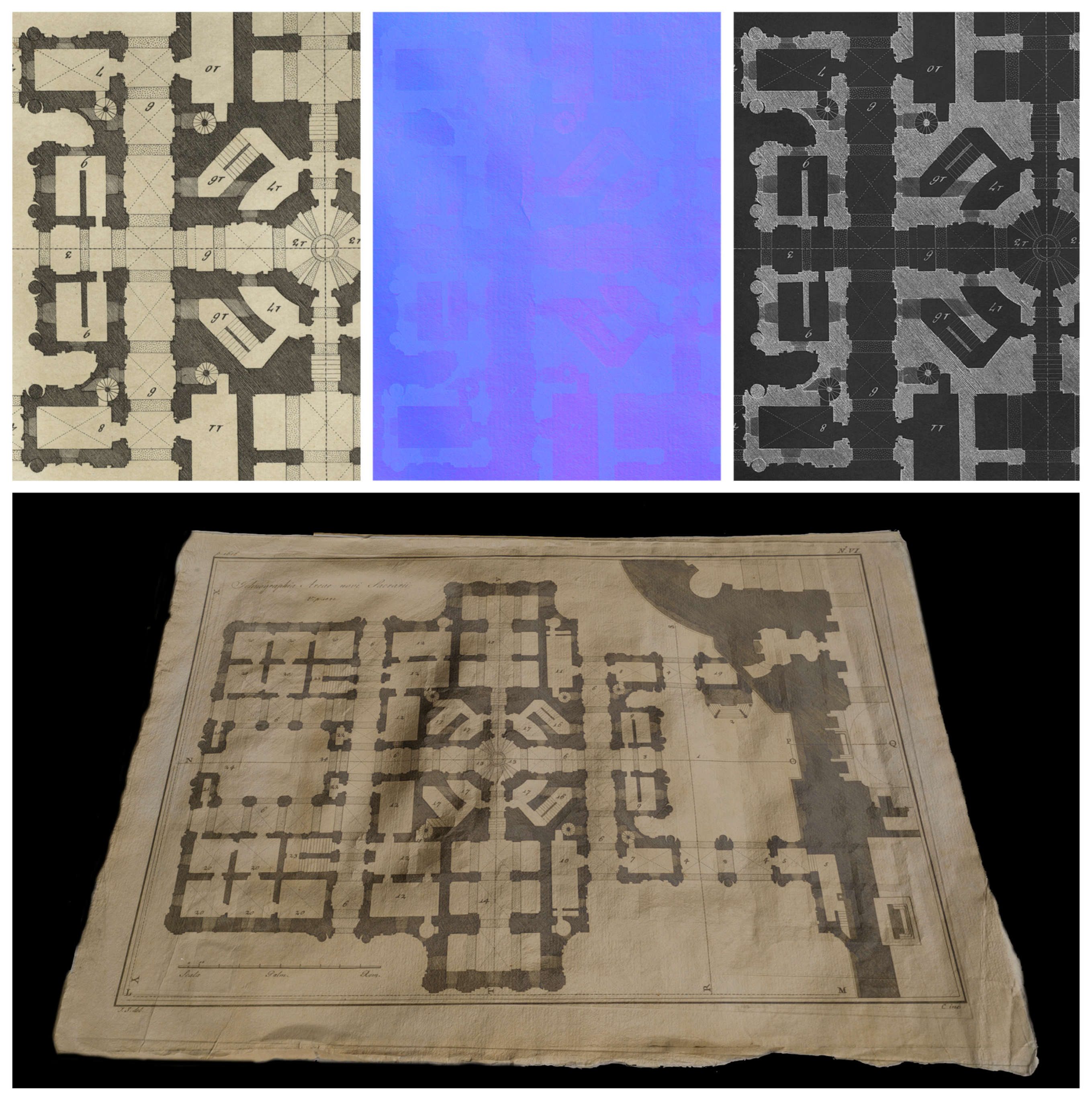
Figure 2.
The mean intensity values (blue) and the standard deviation (red) in the normal map (top) and the mean distances (blue) and the standard deviation (red) of the mesh from a fitting plane (bottom), changing the error in the measurement of the position of the lights along the Z-axis (towards the camera). Both graphs are represented in logarithmic scale.
Figure 2.
The mean intensity values (blue) and the standard deviation (red) in the normal map (top) and the mean distances (blue) and the standard deviation (red) of the mesh from a fitting plane (bottom), changing the error in the measurement of the position of the lights along the Z-axis (towards the camera). Both graphs are represented in logarithmic scale.
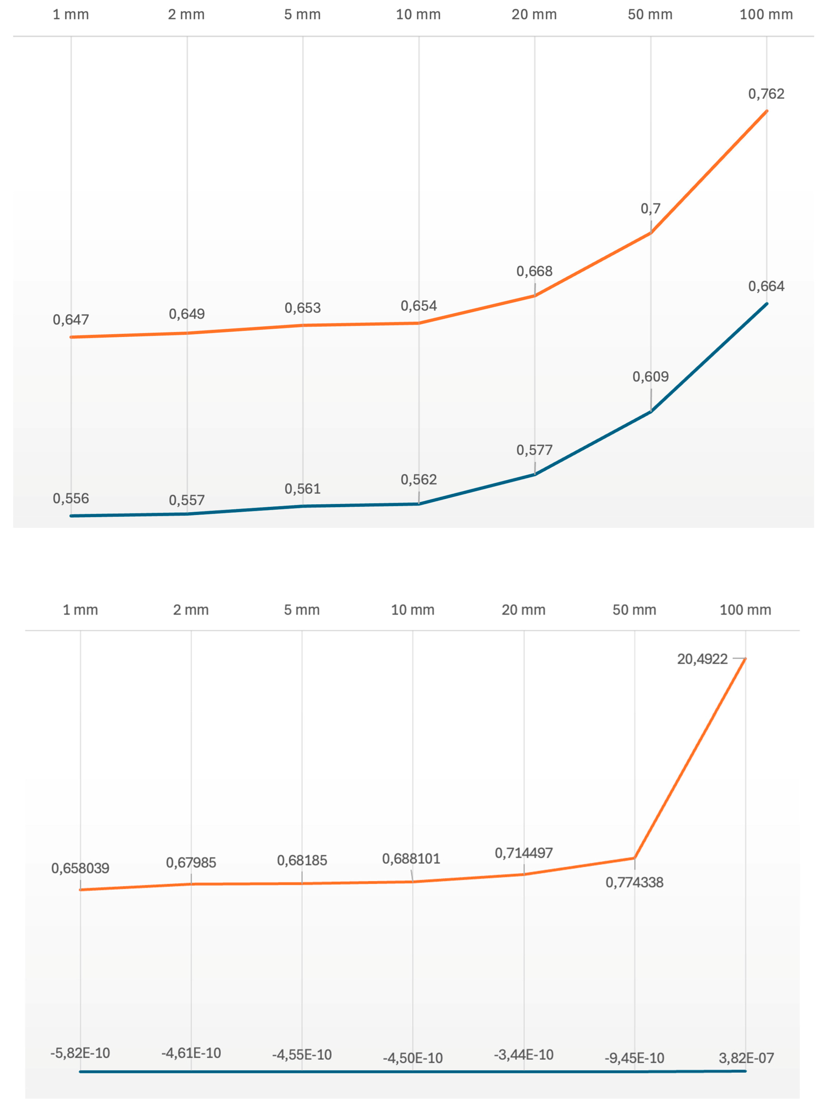
Figure 3.
The horizontal repro stand.
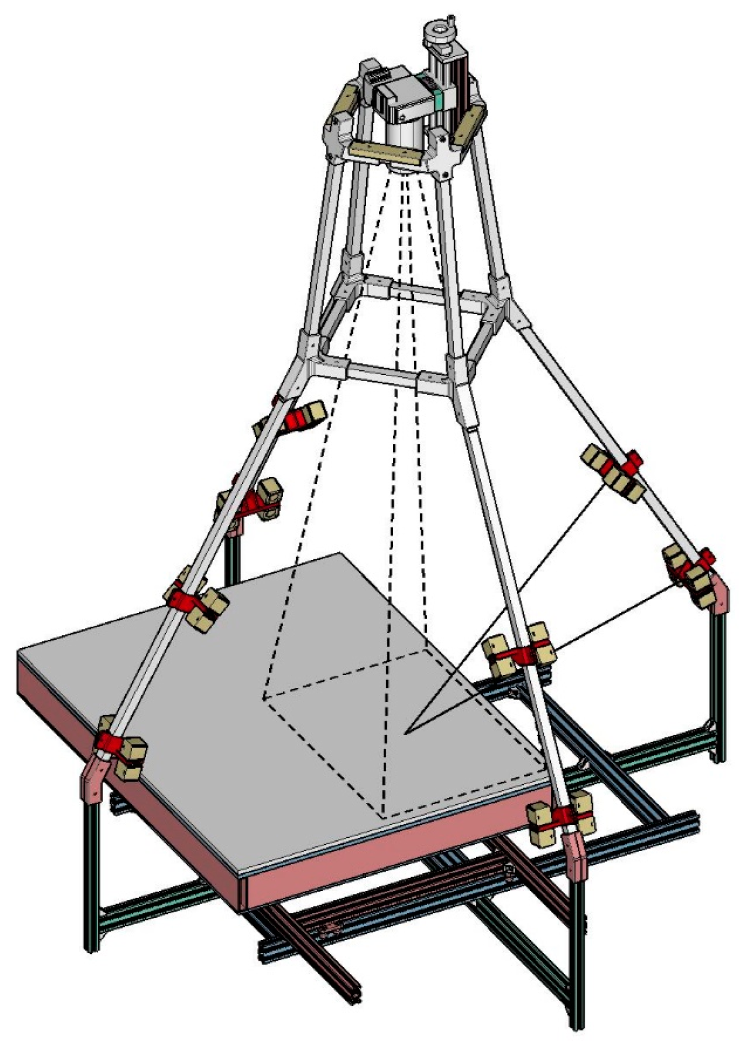
Figure 4.
The elements of the horizontal repro stand: the lower frame (left) and the upper vertical frame (right).
Figure 4.
The elements of the horizontal repro stand: the lower frame (left) and the upper vertical frame (right).
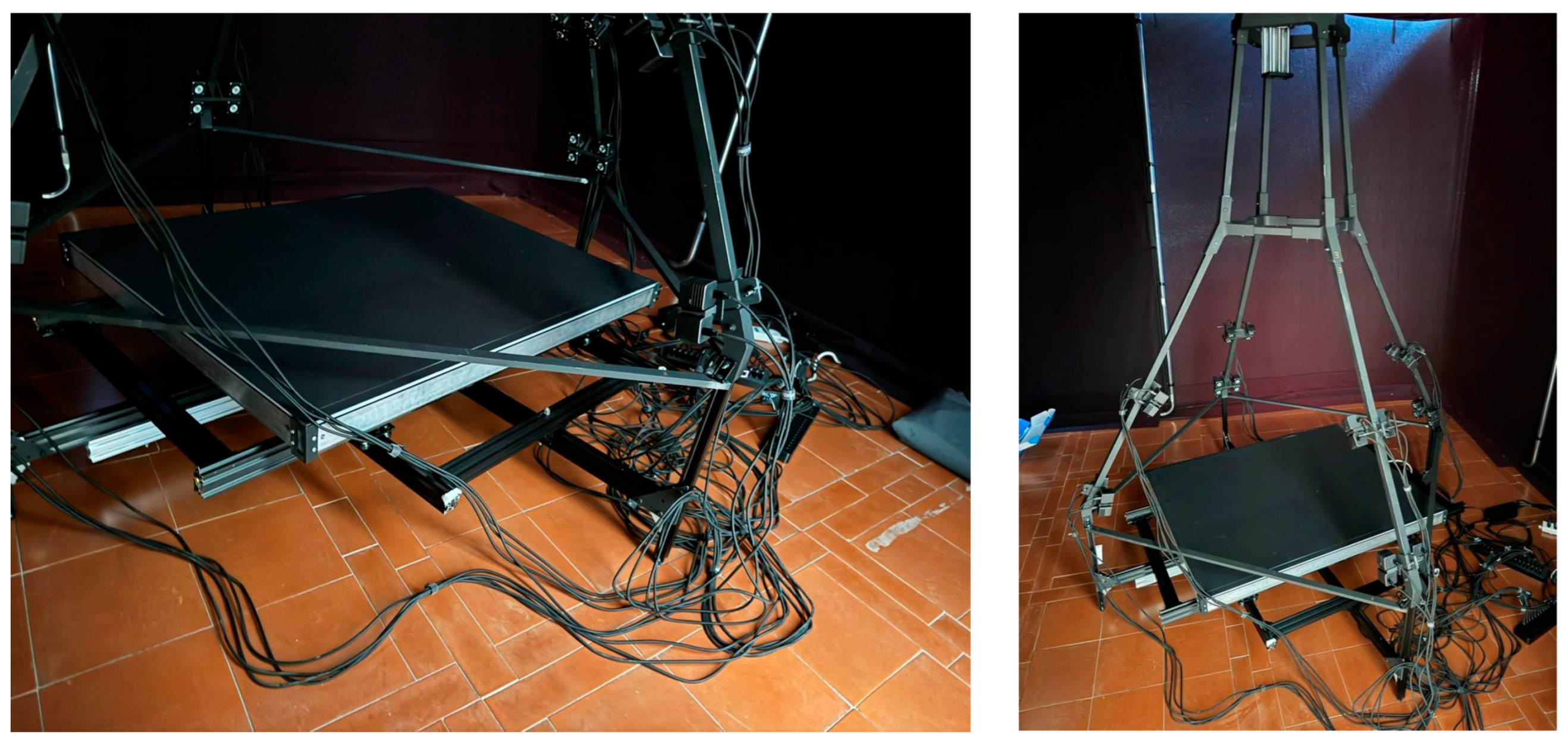
Figure 5.
The robotized vertical repro stand.
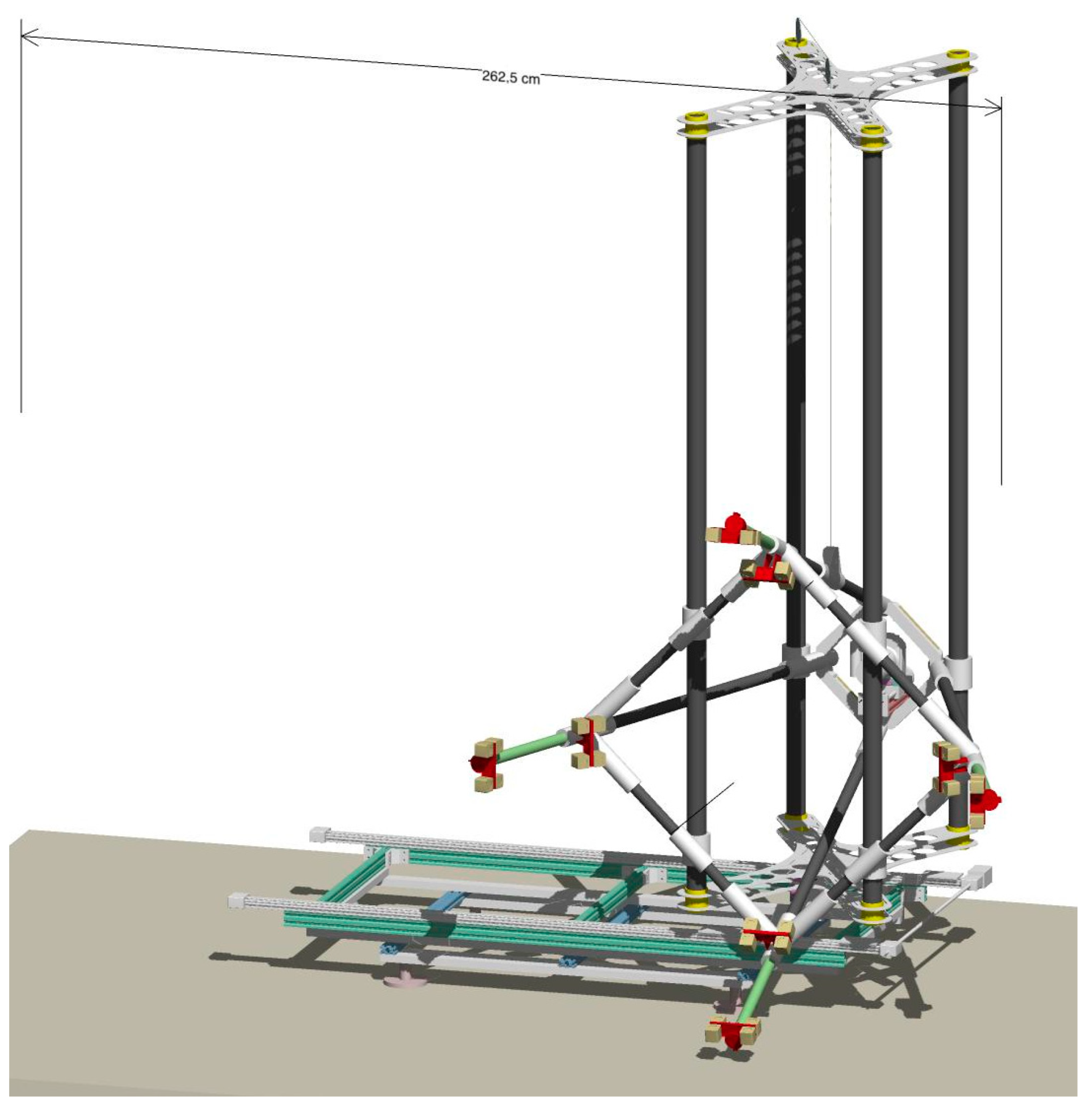
Figure 6.
The elements of the vertical stand main structure: lower frame (left), vertical frame (middle), trapezoidal frame (right).
Figure 6.
The elements of the vertical stand main structure: lower frame (left), vertical frame (middle), trapezoidal frame (right).
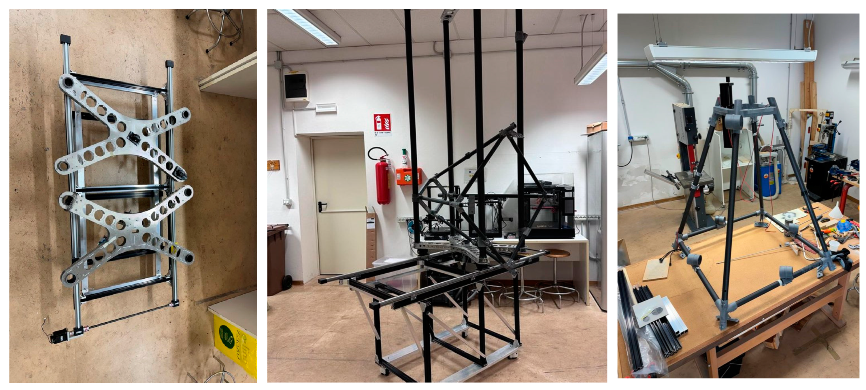
Figure 7.
The darkening occlusion system of the vertical stand.
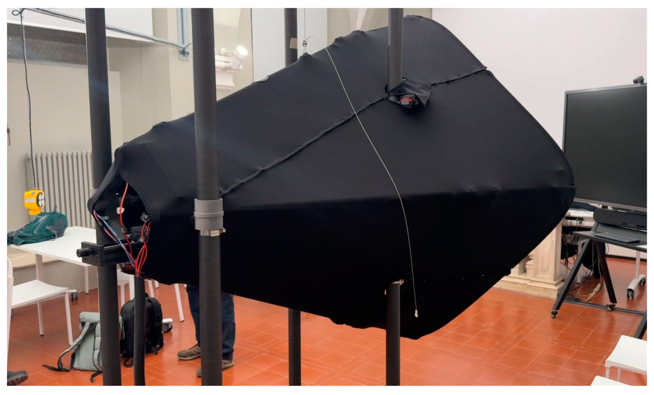
Figure 8.
Origin of typical uncertainties in optical 3D imaging systems.
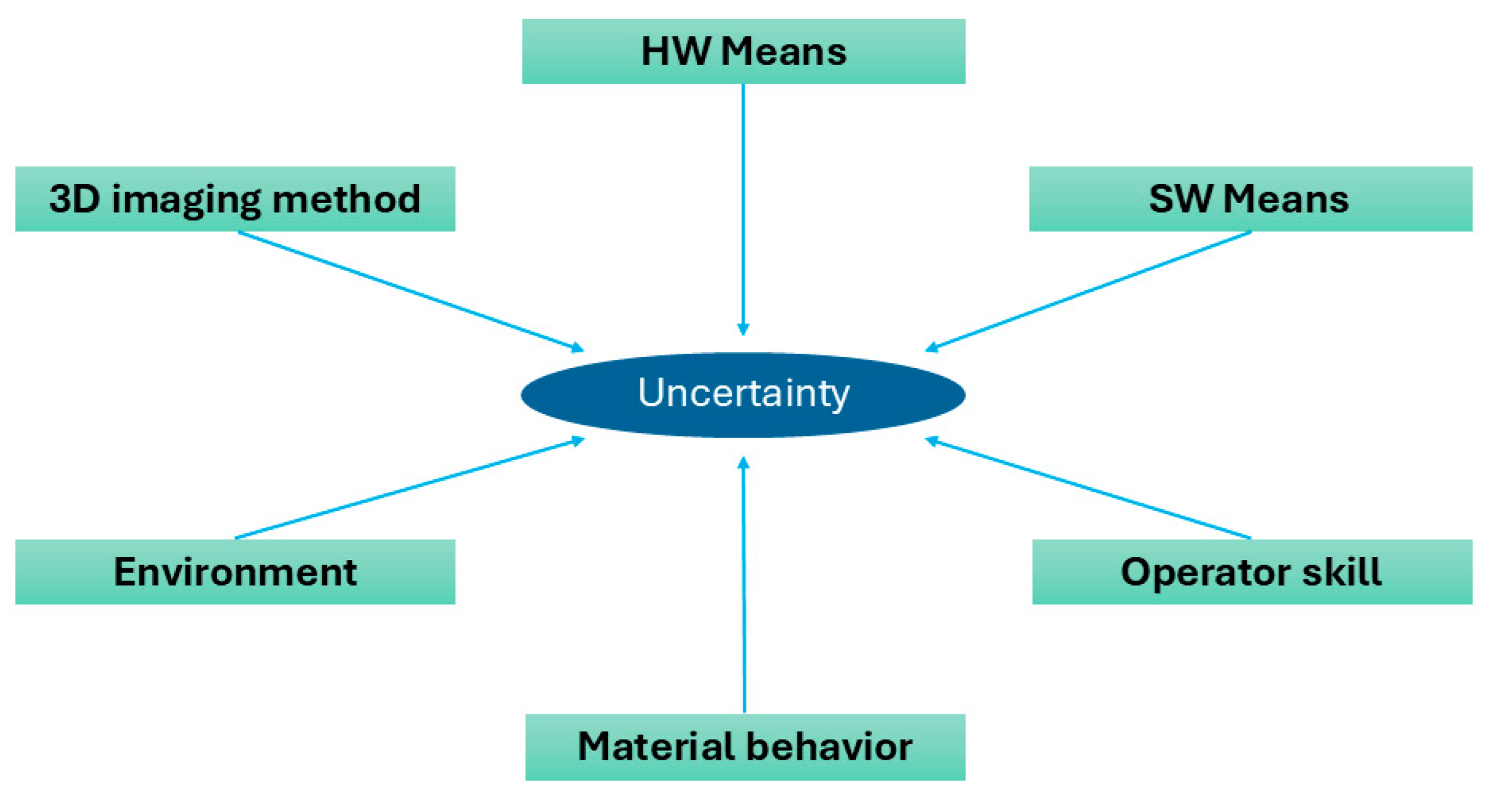
Figure 9.
Workflow of the measurement process.
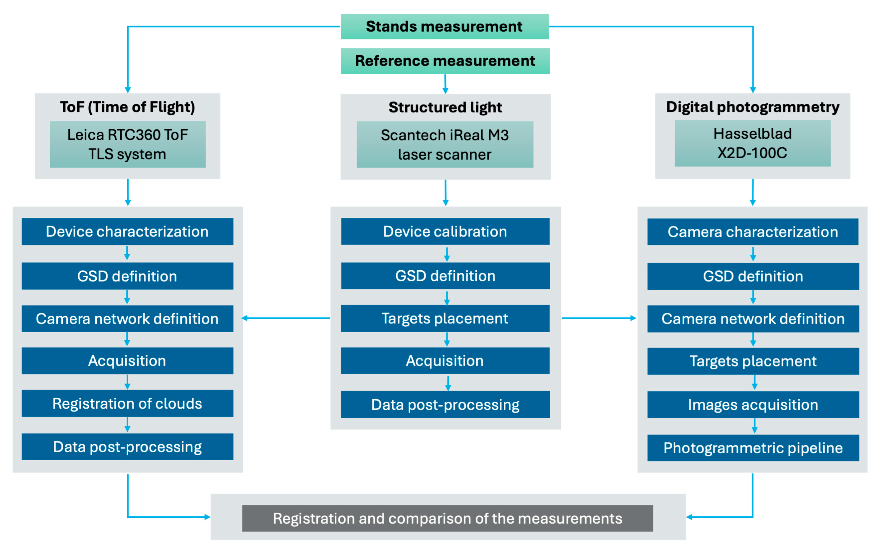
Figure 10.
Schematics for WFD technology [91].
Figure 10.
Schematics for WFD technology [91].
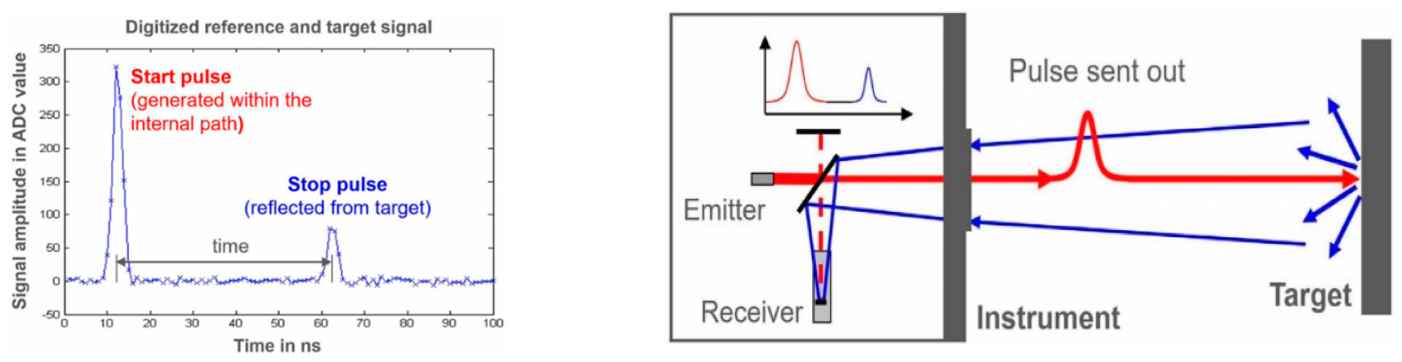
Figure 11.
The glass panel used for the laser scanner characterization.
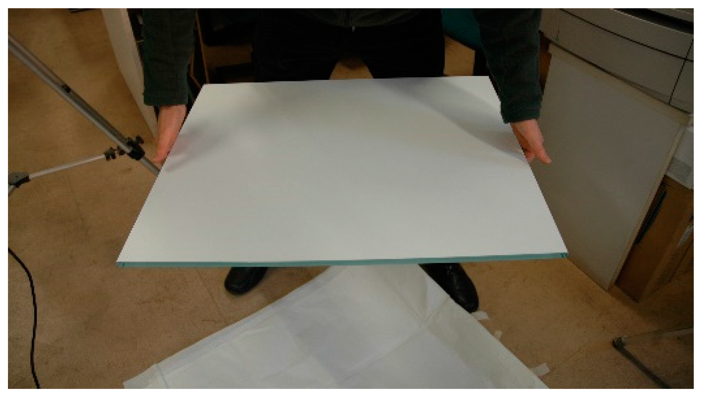
Figure 12.
Point distribution errors of the cloud-to-fitting plane distances of the Scantech iReal M3 (distances are in mm).
Figure 12.
Point distribution errors of the cloud-to-fitting plane distances of the Scantech iReal M3 (distances are in mm).
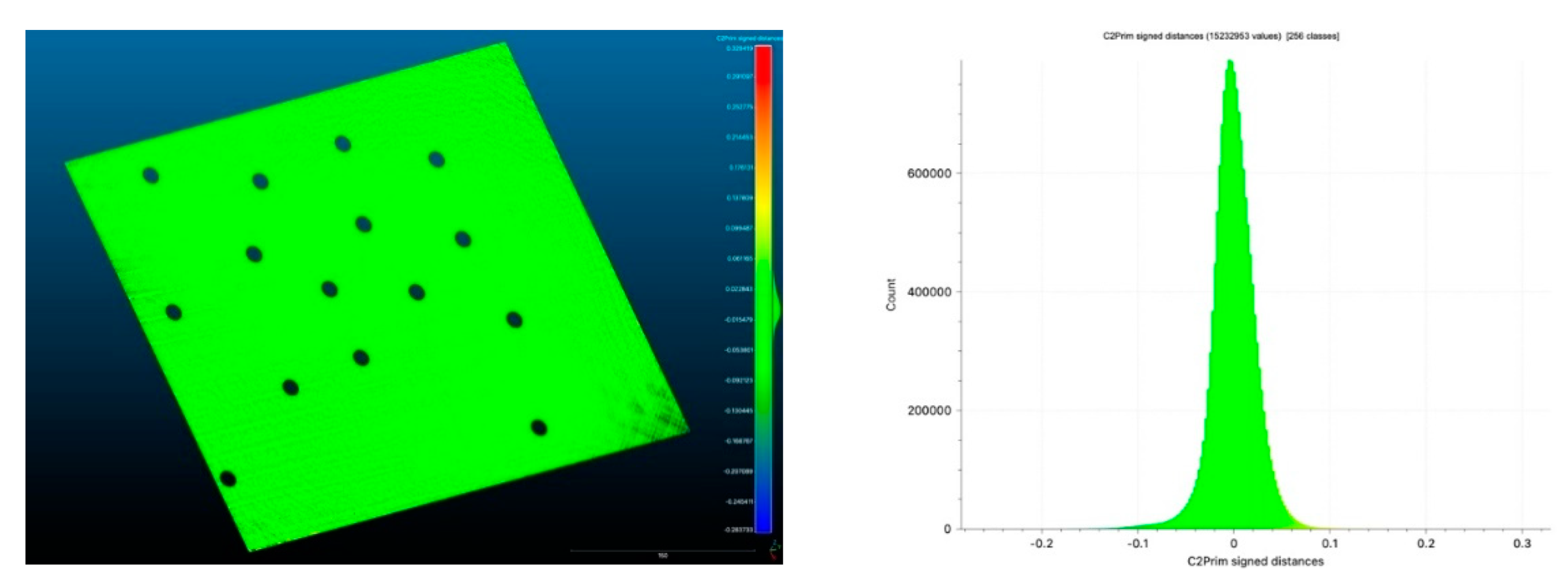
Figure 13.
Point distribution errors of the cloud-to-fitting plane distances of the Leica RTC360 (distances are in mm).
Figure 13.
Point distribution errors of the cloud-to-fitting plane distances of the Leica RTC360 (distances are in mm).
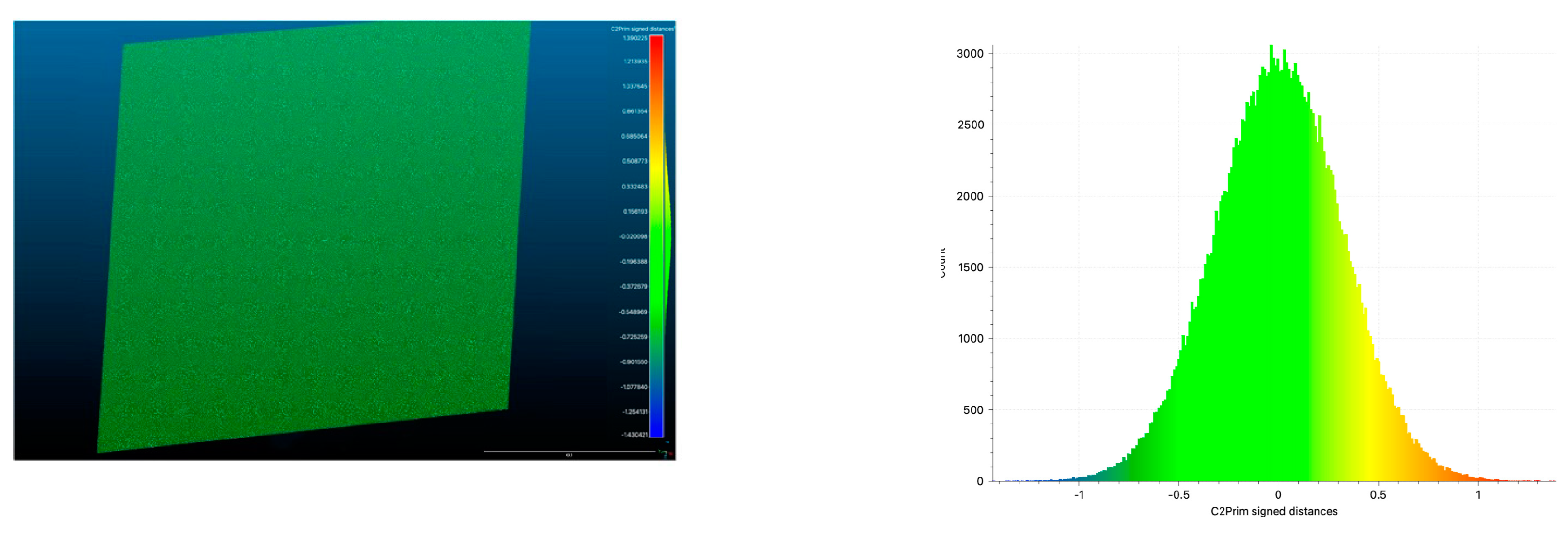
Figure 14.
Image residuals for used Hasselblad X2D-100C camera with XCD 38mm f/2.5 V lens.
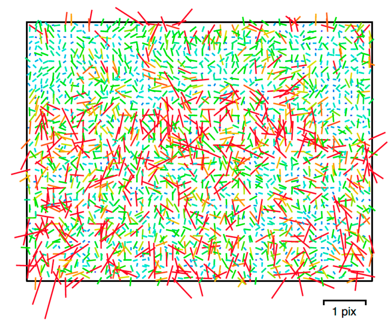
Figure 15.
Vertical plane with the coded RAD targets.
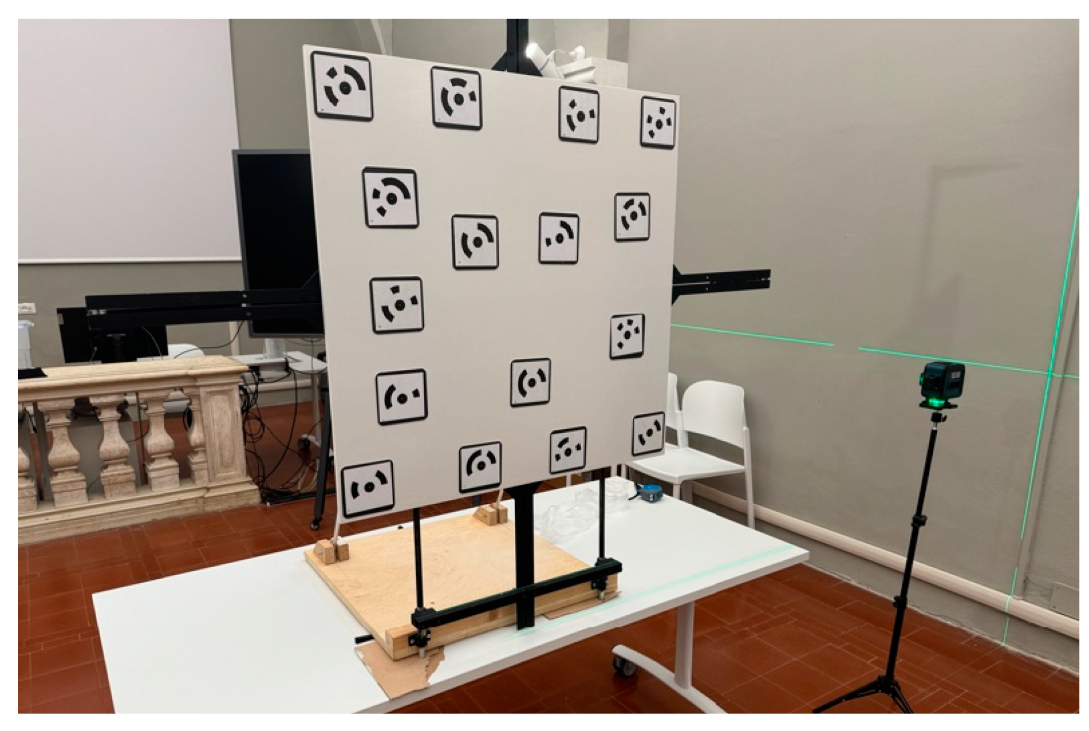
Figure 16.
Radial camera network for the horizontal (left) and vertical (right) repro stands.
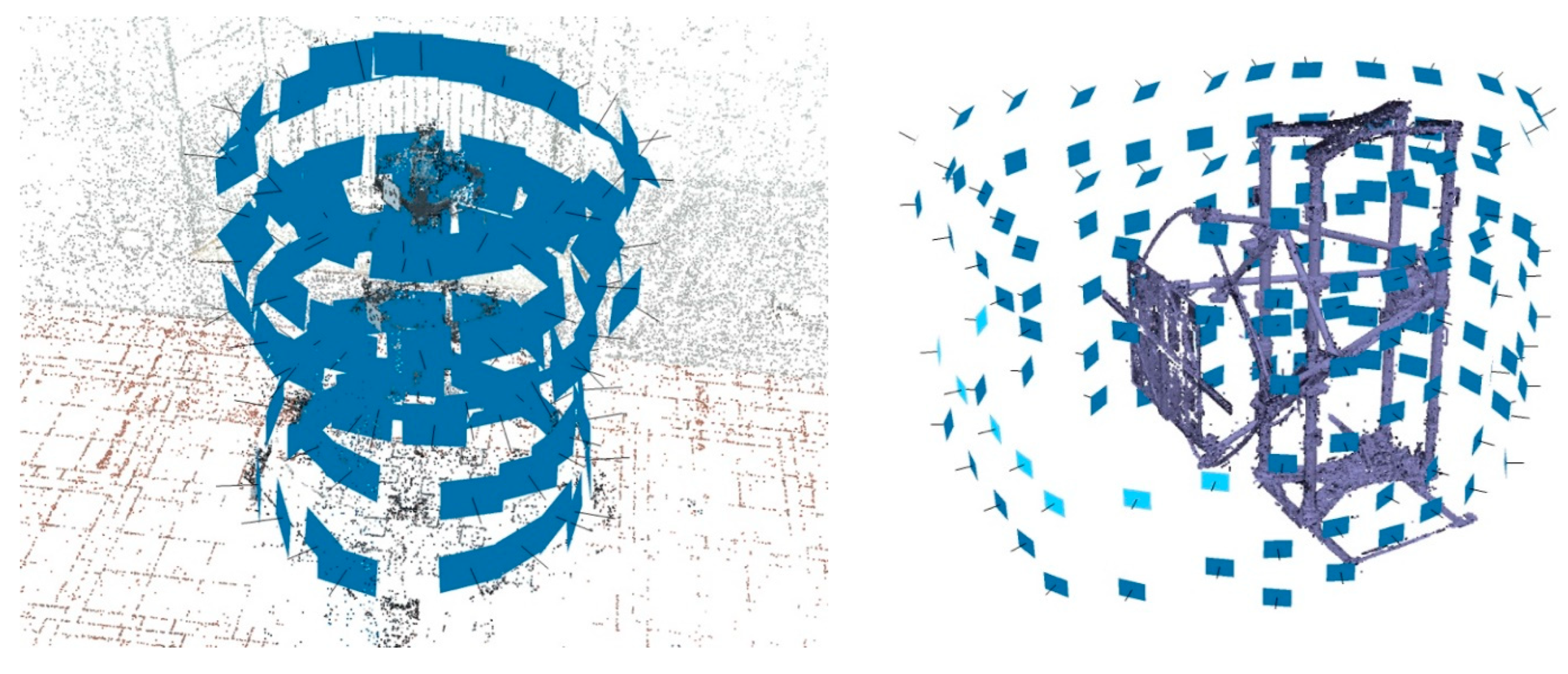
Figure 17.
Shots coverage for the horizontal (left) and vertical (right) repro stands.
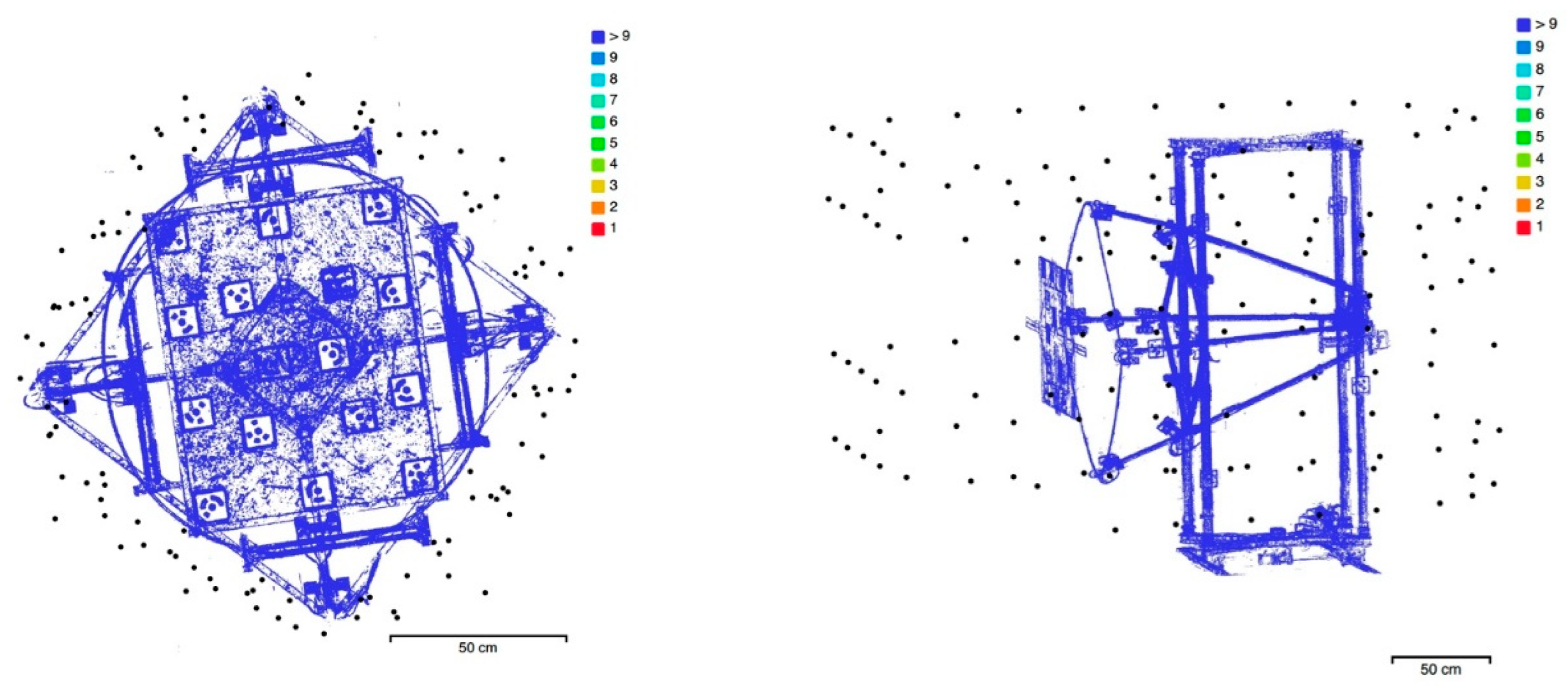
Figure 18.
Point distribution errors of the cloud-to-cloud distances between ToF TLS system and photogrammetry (distances are in mm).
Figure 18.
Point distribution errors of the cloud-to-cloud distances between ToF TLS system and photogrammetry (distances are in mm).
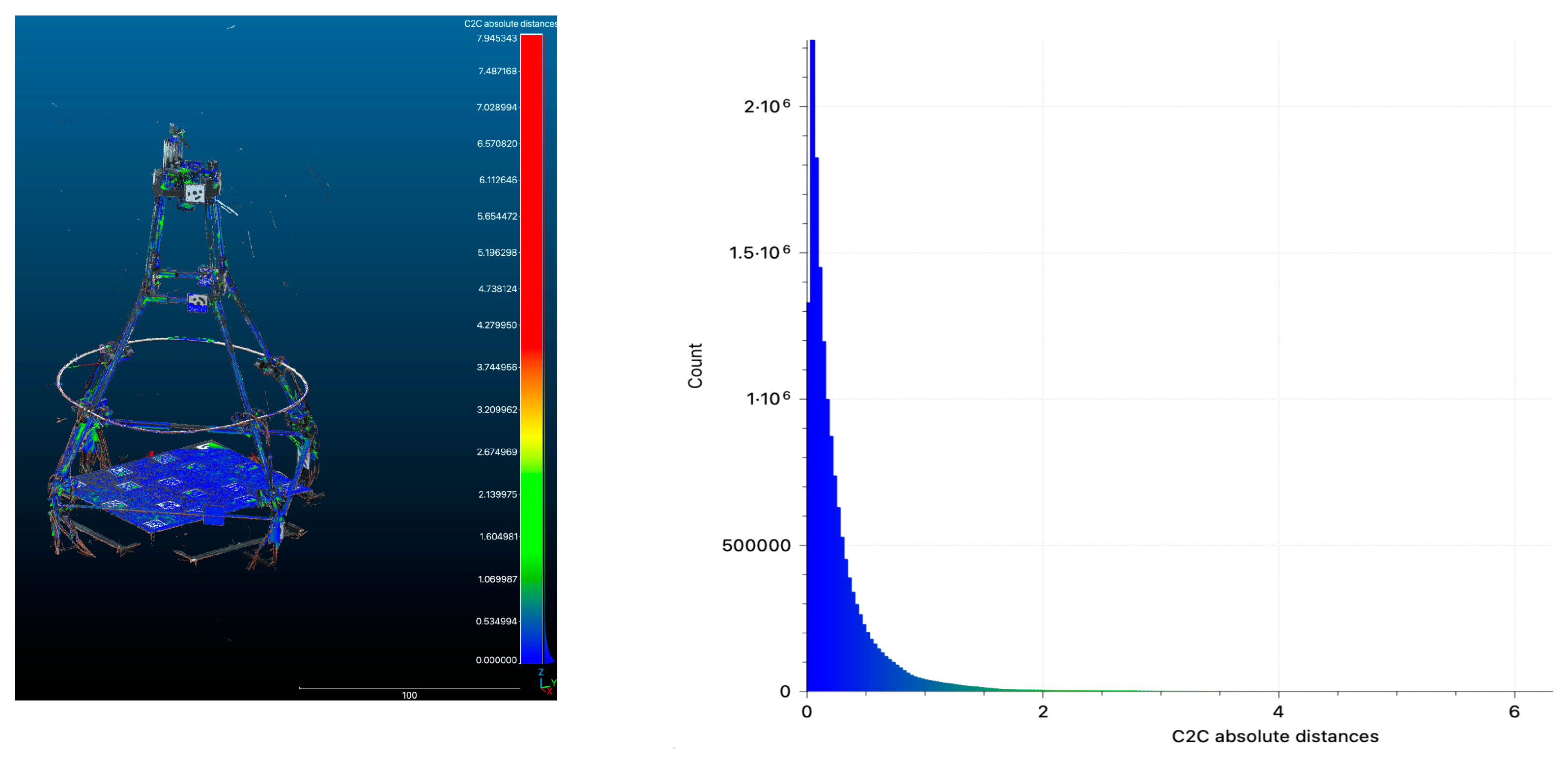
Figure 19.
PoI identification through vector construction on dense cloud points.
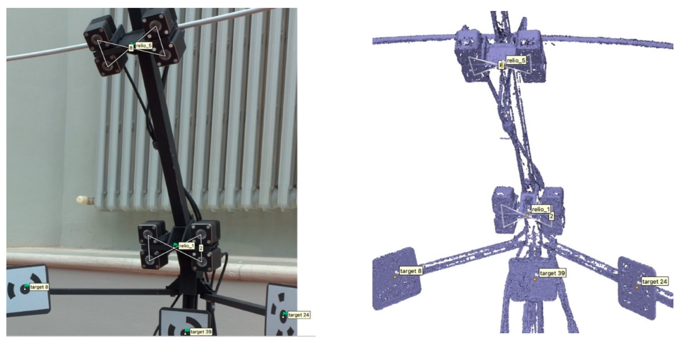
Figure 20.
Point distribution errors of the cloud-to-cloud distances between the ToF TLS system and photogrammetry (distances are in m).
Figure 20.
Point distribution errors of the cloud-to-cloud distances between the ToF TLS system and photogrammetry (distances are in m).
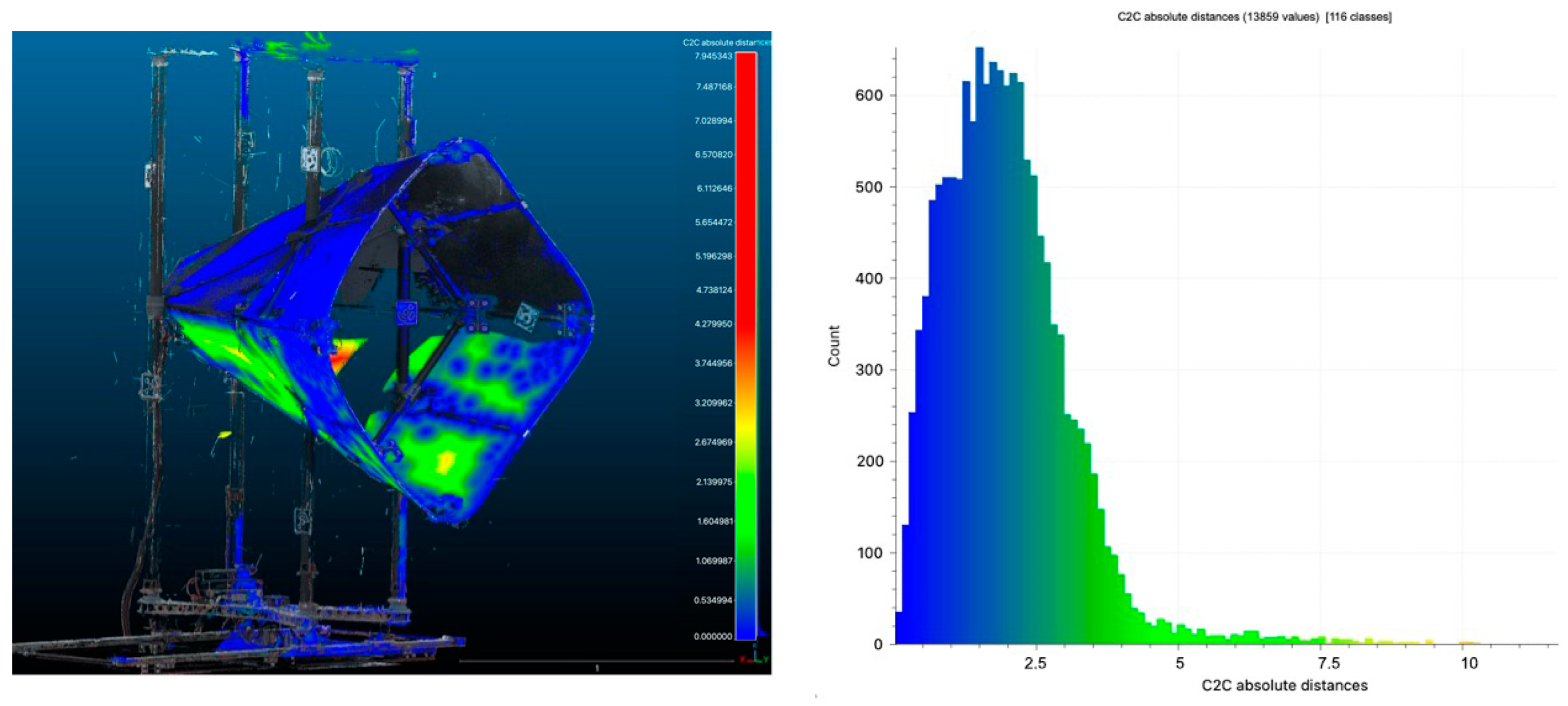
Figure 21.
Point distribution errors of the cloud-to-cloud distances between ToF TLS system and photogrammetry (distances are in mm).
Figure 21.
Point distribution errors of the cloud-to-cloud distances between ToF TLS system and photogrammetry (distances are in mm).
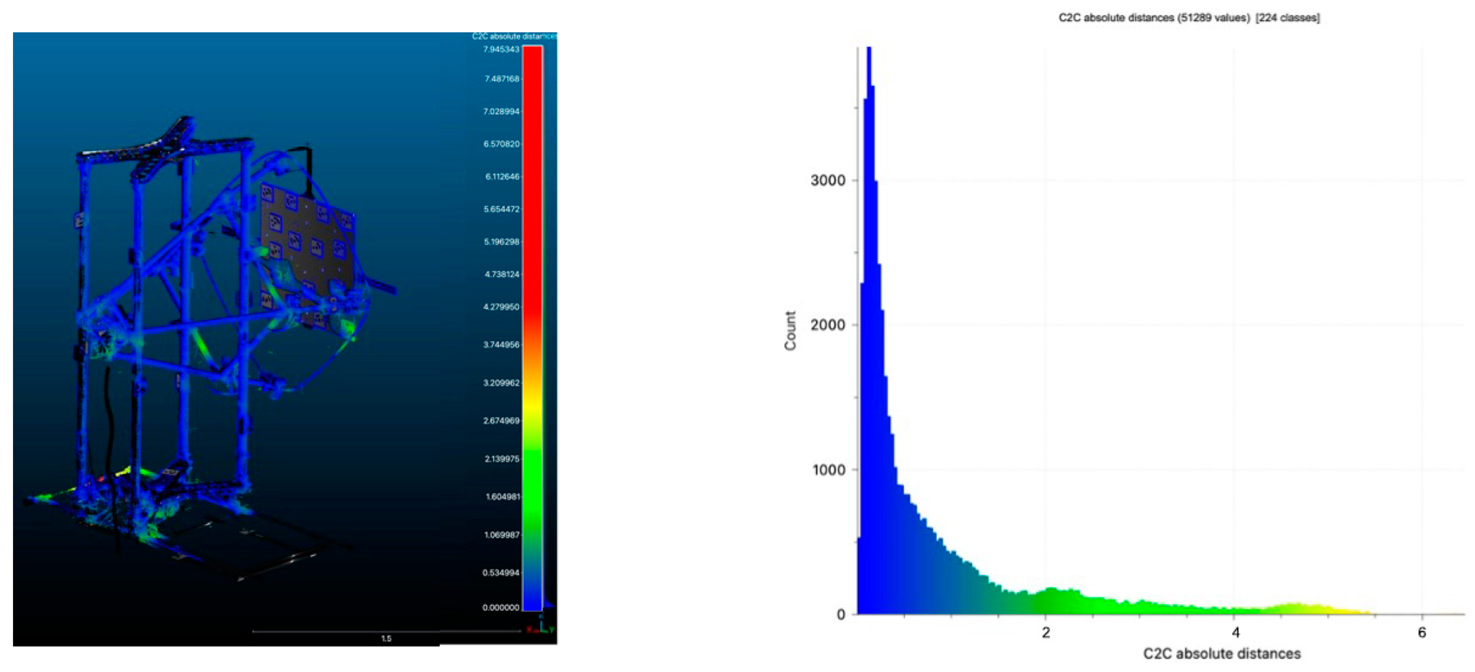
Figure 22.
PoIs identification through vector construction based on dense cloud points.
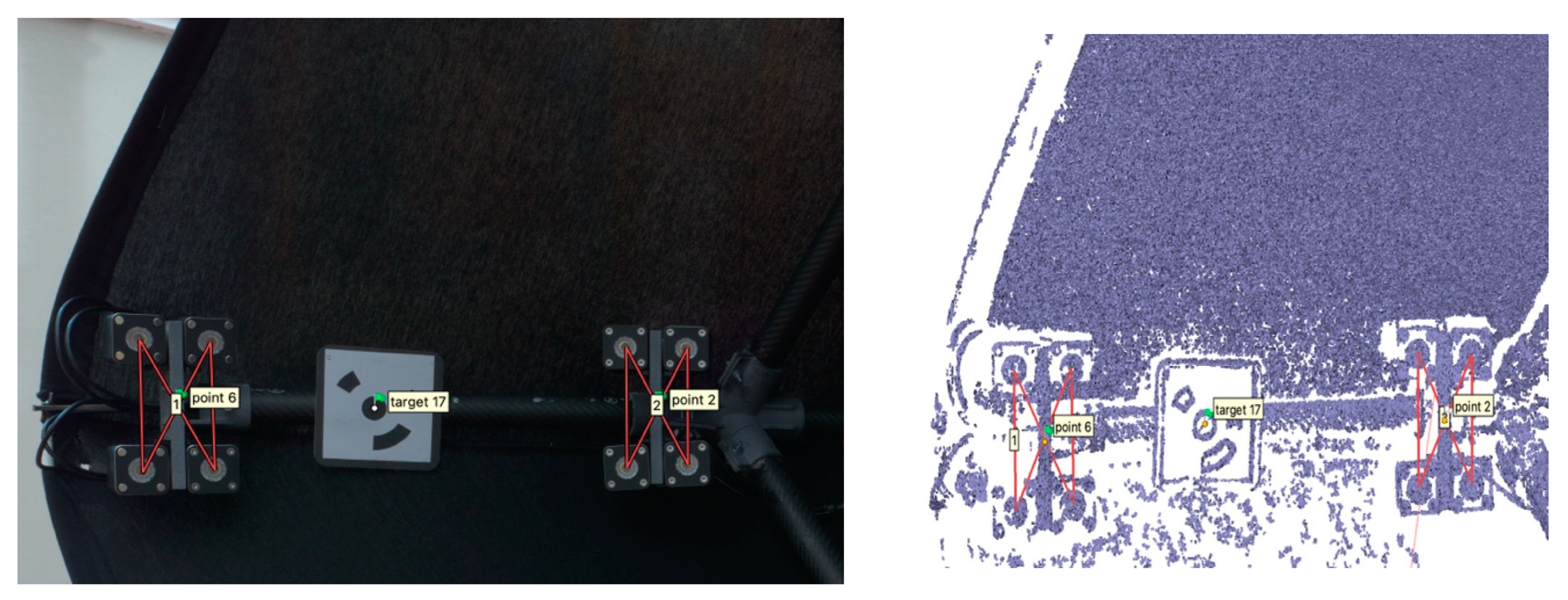
Figure 23.
Comparison between a normal map produced with estimated light directions (left) and our measured ones (right). The horizontal repro stand was adopted.
Figure 23.
Comparison between a normal map produced with estimated light directions (left) and our measured ones (right). The horizontal repro stand was adopted.
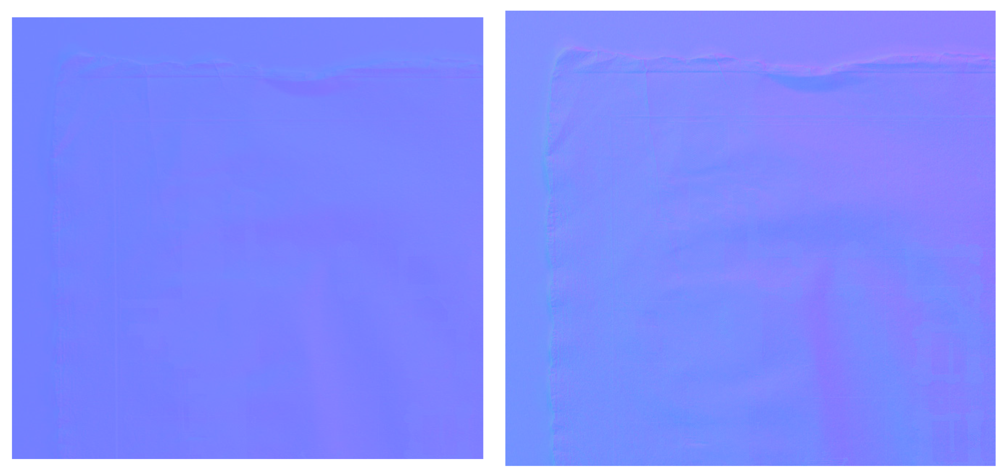
Figure 24.
Comparison of the 3D meshes improved with measured distances (right) and estimated ones (left); the typical “potato chip” effect is fixed. The vertical repro stand was adopted.
Figure 24.
Comparison of the 3D meshes improved with measured distances (right) and estimated ones (left); the typical “potato chip” effect is fixed. The vertical repro stand was adopted.
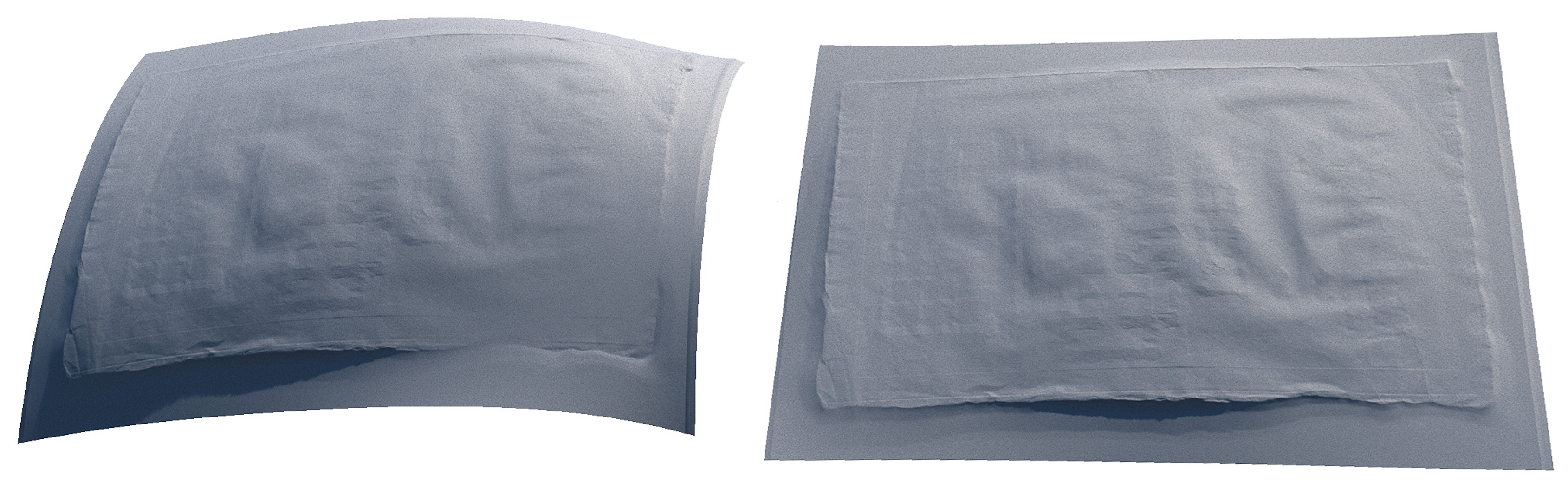
Figure 25.
Comparison of the outcomes of the 3D replication of an old engraving as visualized in the Real-Time Rendering (RTR) engine (Unity, [107]). Maps and meshes from measured stands improve the appearance of the replica (right) much more than the previous solution (left).
Figure 25.
Comparison of the outcomes of the 3D replication of an old engraving as visualized in the Real-Time Rendering (RTR) engine (Unity, [107]). Maps and meshes from measured stands improve the appearance of the replica (right) much more than the previous solution (left).
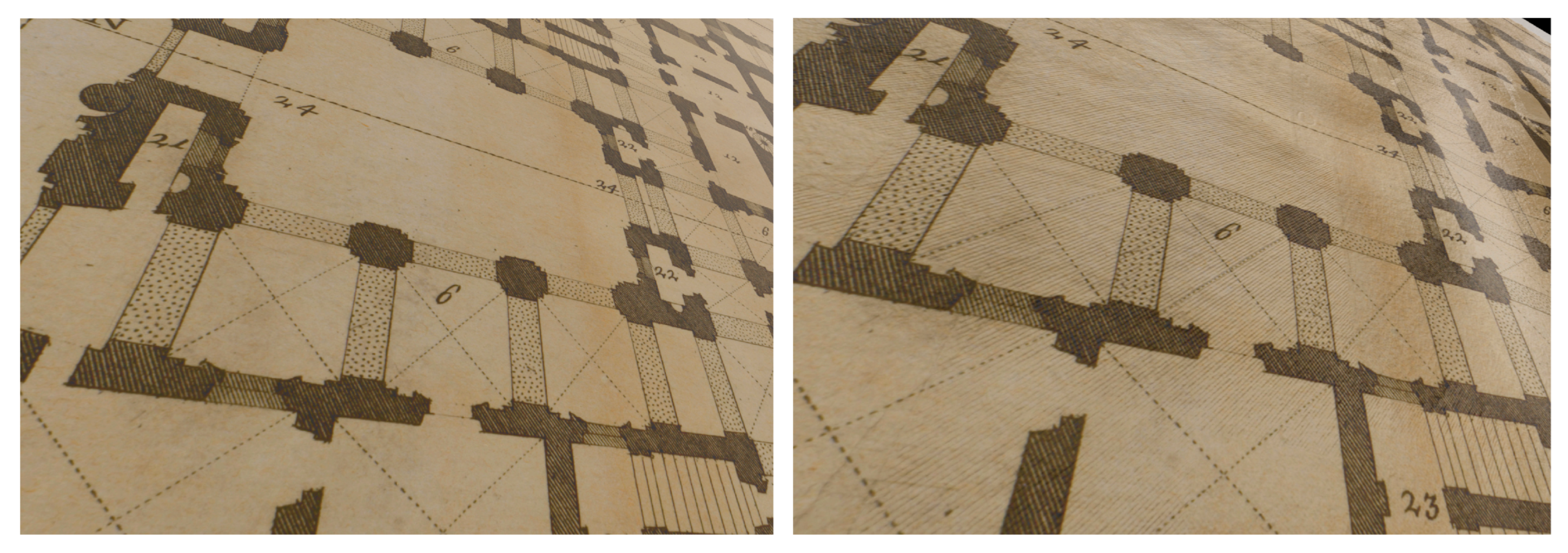
Figure 26.
Comparison of normal maps and 3D meshes of a plane generated for the horizontal stand: without correction (left) and with correction (right). Colors for normal maps are exaggerated for better visibility.
Figure 26.
Comparison of normal maps and 3D meshes of a plane generated for the horizontal stand: without correction (left) and with correction (right). Colors for normal maps are exaggerated for better visibility.
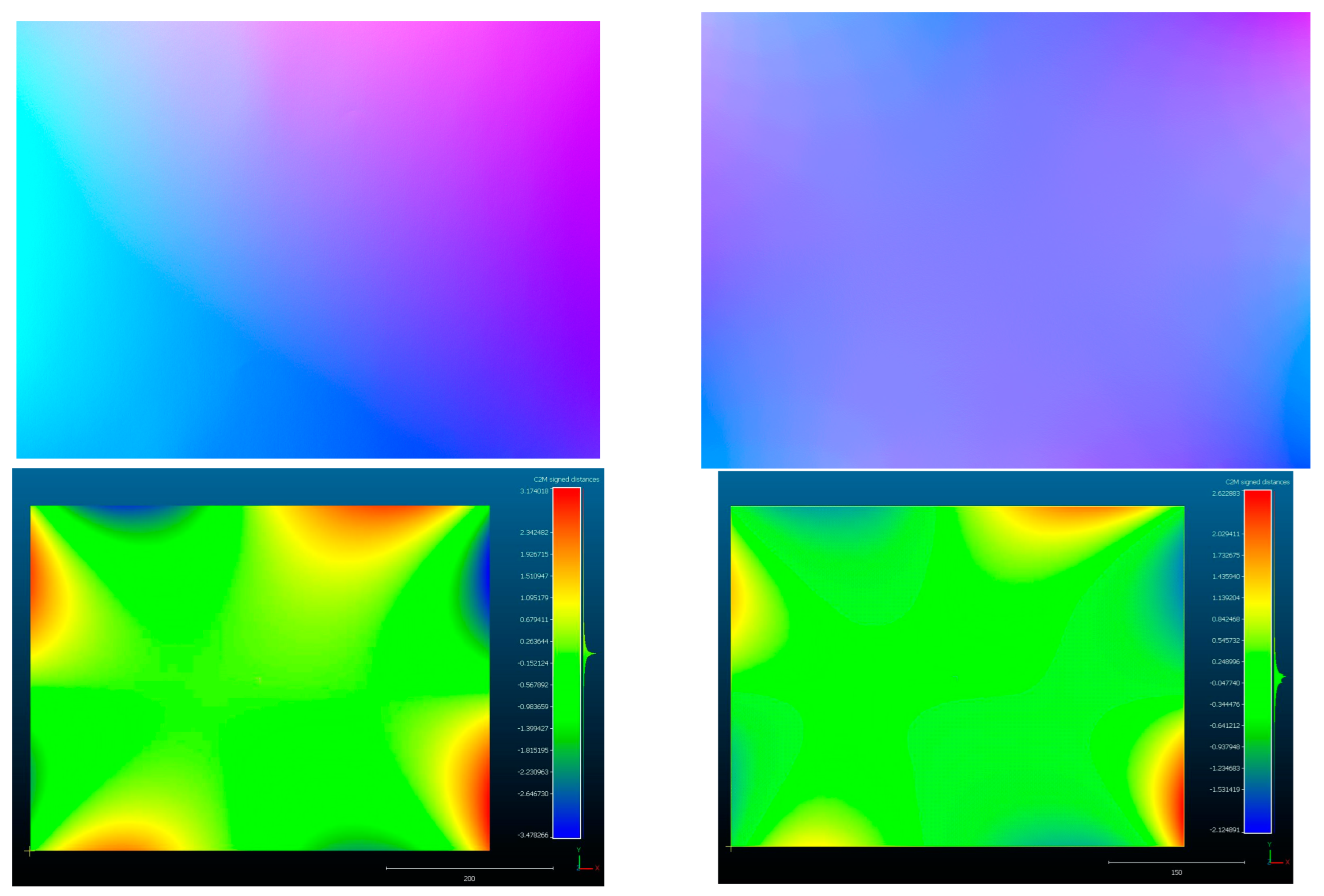

Table 1.
Hasselblad X2D-100C camera.
| Technology | Focus | Resolution | Sensor size | ISO Sensibility | Noise level | Color depth |
|---|---|---|---|---|---|---|
| 100 Megapixel BSI CMOS Sensor | Phase Detection Autofocus PDAF (97% coverage) | 100 megapixel (pixel pitch 3.78 μm) | 11,656 (W) x 8,742 (H) pixel | 64 - 25600 | 0.4 mm a 10 m | 16 bit |
Table 2.
Hasselblad XCD 3,5/120 Macro lens system.
| Focal length | Equivalent focal length | Aperture range | Angle of view diag/hor/vert | Minimum distance object to image plane |
|---|---|---|---|---|
| 120.0 mm | 95 mm | 3.5 - 45 | 26°/21°/16° | 430 mm |
Table 3.
Technical specifications of the Scantech iReal M3 laser scanner.
| Technology | Framed range | Accuracy |
Lateral resolution |
 |
| 7 Parallel infrared laser lines + VCSEL infrared structured light | 580 x 550 mm (DOF 720 mm with an optimal scanning distance of 400 mm) |
0.1 mm | 0.01 mm |
Table 4.
Technical specifications of Leica RTC360 ToF TLS system.
| Technology | Framed range | Accuracy | Resolution | Precision | 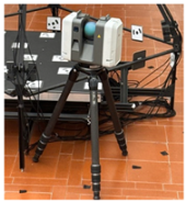 |
| High dynamic ToF with Wave Form Digitizer Technology (WFD) | 360° (H) – 300° (V) | 1.9 mm at 10 m | 3 mm at 10 m | 0.4 mm at 10 m |
Table 5.
Hasselblad XCD 38mm f/2.5 V lens system.
| Focal length | Equivalent focal length | Aperture range | Angle of view diag/hor/vert | Minimum distance object to image plane | 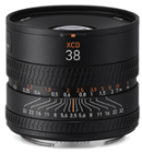 |
| 38.0 mm | 30 mm | 2.5 - 32 | 70°/59°/46° | 300 mm |
Table 6.
Measured precision and accuracy of the Scantech iReal M3.
| Captured Area | 295 x 440 mm |
| Sampled points | 6,130,559 |
| Average distance between a fitted plane and point cloud | 0.000441619 mm |
| Standard deviation | 0.0172472 mm |
Table 7.
Measured precision and accuracy of the Leica RTC360.
| Captured Area | 250 x 500 mm |
| Sampled points | 664,675 |
| Average distance between a fitted plane and point cloud | 0.374145 mm |
| Standard deviation | 0.313806 mm |
Table 8.
Calibration coefficients.
| Value | Error | f | Cx | Cy | b1 | b2 | k1 | k2 | k3 | p1 | p2 | |
| f | 10228.5 | 0.64 | 1.00 | -0.07 | 0.05 | -0.90 | 0.04 | -0.18 | 0.19 | -0.18 | -0.11 | -0.09 |
| Cx | 8.87514 | 0.44 | - | 1.00 | -0.07 | 0.10 | 0.14 | 0.01 | -0.01 | 0.00 | 0.93 | -0.07 |
| Cy | -20.5956 | 0.53 | - | - | 1.00 | -0.21 | 0.08 | 0.03 | -0.03 | 0.03 | -0.09 | 0.72 |
| b1 | -10.4546 | 0.59 | - | - | - | 1.00 | -0.01 | 0.01 | -0.03 | 0.04 | 0.14 | 0.00 |
| b2 | -6.16297 | 0.23 | - | - | - | - | 1.00 | -0.01 | 0.01 | -0.00 | 0.05 | 0.04 |
| k1 | -0.015391 | 0.00023 | - | - | - | - | - | 1.00 | -0.97 | 0.93 | 0.02 | 0.03 |
| k2 | 0.0460376 | 0.0017 | - | - | - | - | - | - | 1.00 | -0.99 | -0.02 | -0.03 |
| k3 | -0.114143 | 0.0048 | - | - | - | - | - | - | - | 1.00 | 0.02 | 0.03 |
| p1 | 0.000138551 | 0.000014 | - | - | - | - | - | - | - | - | 1.00 | -0.07 |
| p2 | 0.000219159 | 0.000011 | - | - | - | - | - | - | - | - | - | 1.00 |
Table 9.
Positions of coded targets (origin at the center of the plane, mm).
| ID | X | Y | Z |
|---|---|---|---|
| 1 | -112.1833981 | -265.6449903 | 1.1604001 |
| 2 | -356.9368841 | 27.3719204 | 1.1928803 |
| 3 | 218.4486223 | 167.6946044 | 0.7668501 |
| 4 | -83.5303045 | 335.2168791 | 0.8040630 |
| 5 | -356.2072197 | -267.7837971 | 1.4174284 |
| 6 | 422.8374003 | 36.3053955 | 0.8180338 |
| 7 | 418.5192553 | -267.5176537 | 0.7987372 |
| 8 | 172.0460260 | -268.9918738 | 1.0840074 |
| 9 | -166.6299110 | -121.8379844 | 1.2866903 |
| 10 | 20.7659104 | -72.1971757 | 0.9835656 |
| 11 | 219.4242678 | -120.2348847 | 0.8334230 |
| 12 | 21.4847097 | 100.0491205 | 0.8094964 |
| 13 | 175.3704988 | 336.8665062 | 0.7985485 |
| 14 | 421.7712423 | 327.9472855 | 1.4888459 |
| 15 | -357.4699748 | 331.4955047 | 0.9538767 |
| 16 | -163.2943198 | 169.2829513 | 0.7963140 |
Table 10.
Photogrammetry point cloud outcomes.
| Agisoft Metashape Professional | Colmap | |
|---|---|---|
| Number of registered images | - | 132 |
| Number of tie points | - | 27,951 |
| Mean observations per image | - | 859,106 |
| Number of points in the dense cloud | 10,367,336 | - |
| RMS reprojection error | - | 0.485 px |
Table 11.
Comparison between ToF TLS and photogrammetry.
| Average distance of points | 0.5214 mm |
| Standard deviation | 0.77006 mm |
Table 12.
PoIs extracted and transformed coordinate values (mm).
| PoI | X | Y | Z |
| Origin | 0 | 0 | 0 |
| Relio_1 | -646.79 | 3.0601 | 171.98 |
| Relio_2 | -3.6600 | 643.86 | 166.24 |
| Relio_3 | 641.34 | 0.3800 | 163.33 |
| Relio_4 | -5.1200 | -645.04 | 165.76 |
| Relio_5 | -474.21 | 2.6700 | 471.77 |
| Relio_6 | 0.1300 | 476.28 | 459.22 |
| Relio_7 | 466.87 | 0.0700 | 467.11 |
| Relio_8 | -5.3300 | -485.74 | 442.38 |
| Camera | 0.0600 | 0.2602 | 1542.48 |
Table 13.
Positions of coded targets (origin at the center of the plane, mm).
| ID | X | Y | Z |
| 1 | -91.7384979 | -254.3196531 | 0.9266232 |
| 2 | -318.6724500 | 98.8737499 | 0.9983411 |
| 3 | 161.4589829 | 252.5450786 | 1.0497326 |
| 4 | 319.6547597 | -319.3383336 | 1.0325548 |
| 5 | -324.2391213 | -105.5458775 | 0.8632963 |
| 6 | 102.4372316 | -79.8087193 | 0.8986234 |
| 7 | -170.2707334 | 252.3647593 | 1.4474652 |
| 8 | -319.6547597 | 319.3383336 | 1.3325548 |
| 9 | 95.2218163 | 96.9329011 | 1.1688642 |
| 10 | 146.1604507 | -261.1907211 | 0.9117996 |
| 11 | -168.9669076 | -16.3564388 | 1.2615517 |
| 12 | 322.6046628 | 126.2068312 | 0.9887015 |
| 13 | -8.7779598 | 248.4658266 | 1.2592235 |
| 14 | -313.2096315 | -327.6061740 | 1.1325548 |
| 15 | 319.9531910 | 319.3383336 | 1.1325548 |
| 16 | 317.9581155 | -126.1577396 | 0.8518509 |
Table 14.
Point cloud outcomes from photogrammetry (with darkening fabric occlusion).
| Agisoft Metashape Professional | Colmap | |
| Number of registered images | 102 | |
| Number of tie points | 70.221 | |
| Mean observations per image | - | 1,099.99 |
| Number of points in the dense cloud | 11,373,875 | - |
| RMS reprojection error | - | 0.465 px |
Table 15.
Point cloud outcomes from photogrammetry (without darkening fabric occlusion).
| Agisoft Metashape Professional | Colmap | |
| Number of registered images | - | 133 |
| Number of tie points | 118,213 | - |
| Mean observations per image | - | 2,990.75 |
| Number of points in the dense cloud | 12,054,708 | - |
| RMS reprojection error | - | 0.499 px |
Table 16.
Comparison between ToF TLS and photogrammetry (with darkening fabric occlusion),.
| Average distance of points | 0.5218 mm |
| Standard deviation | 0.79912 mm |
Table 17.
Comparison between ToF TLS and photogrammetry (without darkening fabric occlusion).
| Average distance of points | 0.4924 mm |
| Standard deviation | 0.69464 mm |
Table 18.
PoIs extracted and transformed coordinate values (mm - with darkening fabric occlusion).
| PoI | X | Y | Z |
| Origin | 0 | 0 | 0 |
| Relio_1 | 10.7631 | -225.7121 | 601.7119 |
| Relio_2 | 605.4825 | -226.7232 | -4.3642 |
| Relio_3 | 7.4924 | -239.9226 | -609.6511 |
| Relio_4 | -603.3234 | -230.8313 | 1.2631 |
| Relio_5 | 0.3228 | -537.4174 | 472.5922 |
| Relio_6 | 461.0301 | -537.3921 | 8.2132 |
| Relio_7 | 1.5820 | -541.6323 | -456.7912 |
| Relio_8 | -461.62 | -537.2876 | 8.1521 |
| Camera | 0.0323 | -1543.8149 | 0.0101 |
Table 19.
PoIs extracted and transformed coordinate values (mm - without darkening fabric occlusion).
Table 19.
PoIs extracted and transformed coordinate values (mm - without darkening fabric occlusion).
| PoI | X | Y | Z |
| Origin | 0 | 0 | 0 |
| Relio_1 | -1.8714 | -235.8112 | 611.5131 |
| Relio_2 | 607.6222 | -225.0312 | -0.5913 |
| Relio_3 | 11.6712 | -238.3611 | -624.8112 |
| Relio_4 | -589.1021 | -223.7463 | -2.9221 |
| Relio_5 | -2.9265 | -543.3825 | 469.5811 |
| Relio_6 | 460.6141 | -538.2921 | 8.1423 |
| Relio_7 | 4.6122 | -539.5241 | -463.3921 |
| Relio_8 | -458.0721 | -533.0126 | 8.1811 |
| Camera | 0.04 | -1543.3821 | 0.1712 |
Table 20.
PoI variation (after assembling the darkening fabric occlusion).
| PoI | X | Y | Z | Euclidean distance |
| Origin | 0 | 0 | 0 | 0 |
| Relio_1 | -12.6345 | -10.0991 | 9.8012 | 18.9125 |
| Relio_2 | 2.1397 | 1.6920 | 3.7729 | 4.6557 |
| Relio_3 | 4.1788 | 1.5615 | -15.1601 | 15.8023 |
| Relio_4 | 14.2213 | 7.0850 | -4.1852 | 16.4304 |
| Relio_5 | -3.2493 | -5.9651 | -3.0111 | 7.4301 |
| Relio_6 | -0.4160 | -0.9000 | -0.0709 | 0.9940 |
| Relio_7 | 3.0302 | 2.1082 | -6.6009 | 7.5629 |
| Relio_8 | 3.5479 | 4.2750 | 0.0290 | 5.5555 |
| Camera | 0.0077 | 0.4328 | 0.1611 | 0.4618 |
Disclaimer/Publisher’s Note: The statements, opinions and data contained in all publications are solely those of the individual author(s) and contributor(s) and not of MDPI and/or the editor(s). MDPI and/or the editor(s) disclaim responsibility for any injury to people or property resulting from any ideas, methods, instructions or products referred to in the content. |
© 2025 by the authors. Licensee MDPI, Basel, Switzerland. This article is an open access article distributed under the terms and conditions of the Creative Commons Attribution (CC BY) license (http://creativecommons.org/licenses/by/4.0/).
Copyright: This open access article is published under a Creative Commons CC BY 4.0 license, which permit the free download, distribution, and reuse, provided that the author and preprint are cited in any reuse.