Submitted:
12 March 2025
Posted:
13 March 2025
You are already at the latest version
Abstract
Understanding and evaluating directed acyclic graphs (DAGs) is crucial for causal discovery, particularly in high-dimensional and small-sample datasets such as microbial abundance data. This study introduces DAGMetrics, an R package designed to evaluate and compare DAGs comprehensively. The package provides descriptive and comparative metrics, streamlining the assessment of outputs from various structure learning algorithms. It was applied to datasets generated for potato tubers and soils from different terroirs (continental and island) and stages (at harvest and post-harvest). Using a comprehensive set of descriptive and comparative metrics, DAGMetrics facilitated model selection by identifying balanced and robust DAGs. PC algorithm with Spearman correlation produced DAGs with moderate complexity and high stability across scaling and transformation setups. Additionally, the package enabled detailed exploration of the Markov blanket space, revealing small Markov blankets (up to 7 nodes) and numerous isolated nodes. Identified matching edges between Markov blankets across different terroirs and stages aligned with known microbial interactions, highlight the package’s utility in facilitating the discovery of biologically meaningful relationships. This study highlights the utility of DAGMetrics in providing objective, reproducible tools for DAG evaluation and its potential application in agronomic and other domains involving complex, structured data.
Keywords:
Agronomic Data Analysis
; Bayesian Networks
; Causal Discovery
; Directed Acyclic Graphs
; Markov Blanket
; Metagenomics
; Microbial Networks
; Structure Learning
1. Introduction
Over the past several years, causal discovery has gained popularity in various fields, including economics [1,2], climate science [3], and biology [4,5,6,7]. More recently, its application has been extended to agronomy. For instance, causal discovery has been successfully employed in proteogenomics to identify cause-and-effect relationships between gene and protein modules [8]. These findings highlight the potential of causal discovery to enhance molecular data exploration and advance the study of key biological processes in plants. Another example is the study of interaction networks in olive leaves, where causal discovery, combining transcriptomic and proteomic data, revealed critical differences between primed and non-primed tissues [9]. Causal discovery is offering a framework to model causal relationships among variables. Unlike traditional statistical methods, which identify associations without specifying the direction of influence, causal models explicitly determine cause-and-effect relationships.
Directed Acyclic Graphs (DAGs) have become powerful tools for representing causal relationships among variables. However, effective evaluation and comparison of DAGs remains a significant challenge across disciplines. As highlighted in [10], it is important to perform DAG evaluation and comparison in a robust manner, as computationally derived causal relationships require further validation across different conditions, datasets, and contexts to ensure their persistence and stability. Similarly, [11] emphasizes the lack of suitable metrics for evaluating DAGs, particularly when the true structure of relationships is unknown.
In microbial data analysis, which is often characterized by high dimensionality and limited sample sizes, ensuring the reliability of model evaluation is a critical concern. Structure learning algorithms can yield significantly different results due to variations in algorithmic approaches and underlying assumptions. The absence of a ground-truth DAG in most real-world applications further complicates the evaluation of these algorithms. While existing tools offer extensive functionality for structure learning, they often lack user-friendly and comprehensive approaches for comparing DAGs or analyzing their local structures in detail. To address these challenges, a tool is needed to systematically compare DAGs by assessing their structural complexity and analyzing differences in local and global structures.
In this paper, we introduce DAGMetrics, an R package designed to facilitate the comprehensive evaluation and comparison of DAGs. The package provides a suite of descriptive and comparative metrics to assess both global and local structures. Descriptive metrics, such as the number of edges and colliders, offer insights into DAG complexity, while comparative metrics evaluate structural similarity. In addition to numerical outputs, DAGMetrics includes visualization tools that enable users to intuitively explore structural differences and similarities.
We demonstrate the functionality of DAGMetrics using real-world agronomic datasets. For example, the package is applied to microbial abundance data collected from potato tubers at harvesting and post-harvesting stages in both island and continental regions. By comparing DAGs learned from these datasets, we uncover differences in microbial interactions and potential causal relationships. The package’s ability to analyze local structures makes it particularly well-suited for agronomic applications and other fields dealing with high-dimensional datasets.
The rest of this paper is organized as follows: In Section 2, we discuss the materials and methods used in this work, including the main concepts of causal discovery, the functionality of the DAGMetrics package, and the preprocessing and statistical analyses applied to the datasets. In Section 3, we present the results, highlighting insights gained and achievements made using the package. Finally, in Section 4, we conclude by summarizing the contributions of this work, its implications for agronomy, and future directions.
2. Materials and Methods
2.1. DAGs, Bayesian Networks, CPDAGs, and Markov Blankets
A DAG is a graph where all edges are directed, and there are no cycles. The absence of cycles ensures that starting from any node and following the direction of the edges, it is impossible to return to the same node. In the context of causal discovery and inference, DAGs encode causal relationships between variables [12]. The absence of an edge between two nodes indicates conditional independence between the corresponding variables, given a specific set of other variables.
DAGs are a powerful framework for representing Bayesian networks, which model the joint probability distribution of a set of random variables [13]. A Bayesian network is defined by a DAG , where V is the set of nodes corresponding to random variables, and E is the set of directed edges that encode conditional dependencies between these variables. If we break down DAGs by triplets of connected nodes and , three main structures can be identified—chains (), forks (), and colliders ()—where the first two exhibit conditional independence between and given , while in a collider, conditioning on induces dependence between and .
A Completed Partially Directed Acyclic Graph (CPDAG) represents a Markov equivalence class of DAGs [4], encoding the same conditional independencies, where directed edges indicate consistent causal relationships across all equivalent DAGs, and undirected edges signify directional uncertainty—for details, refer to Supplementary Material S1.
The Markov blanket of a node in a DAG is the minimal set of nodes, that renders conditionally independent of all other nodes in the graph [2]. In other words, the behavior of a target node can be fully explained by the nodes in its Markov blanket. The Markov blanket of a node consists of its parents, its children, and the other parents of its children. In high-dimensional datasets, such as microbial abundance in potatoes, analyzing the global network may be impractical due to its complexity. Instead, the focus often shifts to specific nodes of interest and their immediate connections, as captured by their Markov blankets.
2.2. Structure Learning and Evaluation
The process of inferring a DAG from data is referred to as structure learning. Structure learning algorithms, including constraint-based methods (e.g., the PC algorithm [12]) and score-based methods (e.g., Tabu Search [14]), aim to uncover underlying causal relationships by leveraging conditional independence tests or optimizing scoring functions. These methods provide the foundation for automated DAG construction and have gained popularity in fields like agronomy, where high-dimensional datasets require advanced methodological tools.
Evaluating DAGs is an important step to assess their structure in terms of complexity and similarity. We distinguish between two categories of metrics: descriptive and comparative.
2.2.1. Descriptive Metrics
Descriptive metrics provide information about the structure and complexity of a DAG. Key metrics include:
- Number of Edges: Measures connectivity and complexity of a DAG.
- Number of Colliders: Counts the number of colliders. In the case of CPDAGs, only edges involved in colliders are typically directed, as they represent causal relationships consistent across all equivalent DAGs. This metric serves as an indicator of the graph’s complexity and the presence of potential causal relationships inferred by the structure learning algorithm.
- Number of Root Nodes: Nodes with no incoming edges.
- Number of Leaf Nodes: Nodes with no outgoing edges.
- Number of Isolated Nodes: Nodes with no connections.
- Degree Metrics: These metrics relate to a specific node, as compared to the full structure. They include in-degree, out-degree, and total degree for nodes, highlighting the importance and connectivity of individual nodes.
2.2.2. Comparative Metrics
Comparative metrics evaluate the similarity between two DAGs. They facilitate the assessment of multiple DAGs to identify similarity in algorithm’s outputs, detect temporal changes in causal structures, or evaluate algorithm performance on synthetic data.
Common metrics include:
- True Positive, False Positive, and False Negative Counts: Identify matches and mismatches in edges between DAGs in counts [24].
These metrics are often scattered across multiple packages, with descriptive metrics missing in many of them. As a result, researchers frequently need to switch between packages—or even programming languages—and manually create custom scripts to achieve a comprehensive evaluation. These fragmented workflows introduce inefficiencies and increase the likelihood of errors.
These limitations underscore the need for a unified tool that integrates descriptive and comparative metrics into a single framework. By streamlining the evaluation process and providing intuitive visualization options, such a tool can eliminate inefficiencies, reduce errors, and enable researchers to focus on extracting meaningful insights rather than dealing with technical challenges.
2.3. DAGMetrics: An R Package for Evaluating and Comparing DAGs
DAGMetrics is an R package designed for the evaluation and comparison of DAGs. It provides a comprehensive suite of descriptive and comparative metrics, covering all the aforementioned metrics for both the global network and the Markov blankets of individual nodes. Additionally, the package includes intuitive visualization features to enhance interpretability and facilitate analysis.
The package offers two primary plotting options:
- Single DAG Visualization: Users can visualize either the full network or the Markov blankets of specified nodes.
- Side-by-Side Comparison: This feature allows for the direct comparison of two DAGs or the Markov blankets of specified nodes. In these visualizations, selected nodes and matching edges between the two DAGs are highlighted in green, making it easier to identify shared structures and differences.
These visualization tools are particularly valuable for focusing on specific areas of interest. Researchers can specify a list of nodes, enabling a targeted examination of local structures. This capability is especially useful in high-dimensional datasets, where analyzing the global network can be overwhelming. By breaking the network into manageable parts, the package enhances interpretability and provides deeper insights into complex datasets.
DAGMetrics is available on GitHub at https://github.com/averinpa/DAGMetrics.
2.4. Data Description and Preprocessing
The DAGMetrics package was applied to two metagenomic datasets: soil and potato tuber microbial diversity from two diverse terroirs, continental (Lakoma, Thessaloniki) and island (Naxos, Aegean Sea). In particular, the tuber dataset represented microbiome data from potato tubers of continental and island terroirs at harvest and post-harvest, essentially as previously described [10]. The soil dataset consisted of soil samples originating from the same contrasting terroirs, Naxos and Lakoma [25]. Raw data were obtained from the National Centre for Biotechnology Information (NCBI) Sequence Read Archive (SRA) under the BioProject accession numbers PRJNA854325 (for the tuber dataset), and PRJNA970975 (for the soil dataset).
After filtering and preprocessing (more details are available in the Supplementary material), six datasets were prepared for both island and continental terroirs. These included combinations of the original, scaled, and transformed versions, ready for further structure learning.
2.5. Model Selection
For the tuber datasets (island and continental terroirs at harvest and post-harvest stages) and the soil datasets (island and continental terroirs), two constraint-based algorithms and two score-based algorithms were applied, each with various hyperparameter settings.
For the constraint-based algorithms, we used the PC algorithm [12] from the pcalg package [26] and the Inter-IAMB [27] algorithm from the bnlearn package [28]. Both algorithms were tested with three different correlation setups for calculating conditional independence tests: Kendall correlation, Spearman correlation, and Pearson correlation. The significance level () for the tests was set to 5%.
For the score-based algorithms, we applied Tabu Search [14] and Hill-Climbing. Prior to applying these algorithms, the data were discretized, following a common approach adopted by other researchers [29,30]. Two scoring metrics, BIC and AIC, were evaluated during the analysis.
This process resulted in a total of 240 DAGs for the tuber dataset, and 120 DAGs for the soil dataset.
The model configurations were encoded as follows: the first letter denotes the algorithm family: C for constraint-based and S for score-based methods. The number following the letter identifies the specific algorithm: C1 corresponds to PC, C2 to Inter-IAMB, S1 to Tabu Search, and S2 to Hill Climbing. The second digit represents the hyperparameter used: 1 for Kendall, 2 for Spearman, and 3 for Pearson for constraint-based algorithms, and 1 for BIC, 2 for AIC for score-based algorithms. The third digit specifies the scaling approach: 1 for no scaling, 2 for Z-score normalization, and 3 for Min-Max scaling. The fourth digit indicates the transformation applied: 1 for no transformation and 2 for rank-based transformation.
The compare_dags function from the DAGMetrics package was used to calculate a comprehensive set of descriptive and comparative metrics to evaluate the resulting DAGs in terms of complexity and similarity.
To assess the complexity of the resulting DAGs, we utilized:
- The normalized number of edges,
- The normalized number of colliders, and
- The normalized number of isolated nodes.
To ensure comparability of DAG across different stages and terroirs, we used normalized descriptive metrics, where normalization was performed by dividing each metric by the number of nodes in a structure. These metrics provide a framework for comparing the complexity of DAGs across different settings.
For similarity evaluation, we employed F1 score, which offers insights into the structural differences and overlaps between DAGs.
The most appropriate algorithm was chosen by selecting DAGs with moderate complexity and stability across different scaling and transformation setups.
2.6. Statistical Analysis
The selected DAGs were utilized to explore the Markov blanket structures within each terroir and stage. This analysis aimed to provide a detailed description of the Markov blanket space and to identify Markov blankets with matching causal relationships across terroirs (island and continent) and stages (harvest and post-harvest).
The compare_dags function from the DAGMetrics package was employed to calculate descriptive metrics for each Markov blanket. These metrics included:
- The number of edges,
- The number of colliders,
- The number of nodes, and
- The number of isolated nodes.
Additionally, matching causal relationships were identified using the true positive count metric, which quantifies the shared causal connections between Markov blankets.
For an in-depth analysis of specific microbes, the vis_dag_comparison function was used. This function facilitated visual comparisons of the Markov blankets of microbes of interest by generating side-by-side network visualizations.
To further enhance the interpretability of the results, network visualizations were created using Cytoscape software [31]. Cytoscape allowed for the customization of network diagrams.
3. Results
In this section, we present the results demonstrating how the DAGMetrics package facilitated the selection of the most appropriate model. This methodology may be of interest to researchers applying causal discovery algorithms to agronomic datasets. Further, the results of detailed analysis of Markov blankets will be presented. Finally, we outline the estimated Markov blankets with matching edges and provide a detailed description of the identified and selected Markov blankets.
3.1. Model Selection
The complexity of the DAGs produced by score-based and constraint-based algorithms varied significantly. The detailed results are presented in Figure 1 for the tuber dataset. The corresponding information for the soil dataset is displayed in Supplementary Figure S1.
On average, score-based algorithms generated denser graphs with more edges, while constraint-based algorithms produced sparser DAGs for both tuber and soil datasets. Additionally, DAGs generated by constraint-based algorithms had a higher proportion of isolated nodes.
Interestingly, the number of colliders showed a mixed pattern: some constraint-based algorithms produced more colliders than score-based algorithms, while others produced fewer. The complexity of DAGs learned by both types of algorithms also varied depending on the hyperparameter settings. For instance, score-based algorithms using the BIC criterion produced less complex structures compared to those using the AIC criterion. Among constraint-based algorithms, those utilizing Kendall correlation yielded the least complex graphs. For example, the structure of continental abundance at the post-harvest stage, learned using the PC algorithm with Kendall correlation, had 75% isolated nodes (Figure 1). Similarly, for the soil dataset, structures learned with the PC algorithm and Kendall correlation resulted in 79% and 85% isolated nodes for island and continental terroirs, respectively (Supplementary Figure S1). Constraint-based algorithms using Spearman and Pearson correlations exhibited medium complexity compared to score-based algorithms and constraint-based algorithms using Kendall correlation. In terms of algorithm stability under different scaling and transformation setups, outputs from the PC and Inter-IAMB algorithms using Spearman and Kendall correlations demonstrated consistent patterns. This trend is observed across both the tuber and soil datasets.
The similarity between DAGs produced by different structure learning algorithms was measured using the F1 score for each dataset. Detailed results for the tuber dataset in the island terroir at the harvest stage are presented in Figure 2, while Supplementary Figures S2 and S3 visualize the corresponding results for other terroirs and stages of the tuber dataset, as well as the soil dataset. The results revealed a high level of dissimilarity between the outputs of score-based and constraint-based algorithms (Figure 2 and Supplementary Figures S2 and S3). Additionally, variations were observed among the outputs of constraint-based algorithms (Figure 2 and Supplementary Figures S2 and S3). For instance, the DAGs learned with the PC algorithm using Pearson correlation differed from those using Spearman or Kendall correlation, as well as from structures produced by Inter-IAMB configurations (Figure 2 and Supplementary Figures S2 and S3).
The PC and Inter-IAMB algorithms using Pearson correlation demonstrated consistency across normalization setups, whereas the same algorithms with Spearman and Kendall correlation exhibited similarity across scaling and transformation setups. Score-based methods showed moderate similarity across different algorithms; however, notable differences were observed across transformation setups.
3.2. Analysis of Markov Blankets
The structures of Markov blankets in the two datasets exhibited both similarities and differences. As shown in Figure 3 for the tuber dataset and in Supplemetary Figure S4 for the soil dataset, most Markov blankets contained no colliders in their structures. However, in the soil dataset, colliders were rare, with only a few instances where a single collider was present and no instances with more than one collider. In contrast, the tuber dataset showed a different pattern, with instances of up to three colliders across terroirs and stages. Notably, in the island terroir, there were even instances with four and six colliders (Figure 3). In the soil dataset, Markov blankets most frequently had no edges, followed by those with one edge, with a few instances of two or three edges. There was a significant gap in the frequency between Markov blankets with no edges and those with one edge (Supplementary Figure S4). In the tuber dataset, particularly in continental terroir, Markov blankets with no edges were predominant, but the gap between those with no edges and one edge was smaller compared to the soil dataset. In the island tuber dataset, Markov blankets with one edge were more frequent than those with no edges. Markov blankets with two edges were slightly less frequent than those with one edge, although in continental post-harvest, their frequencies were similar (Figure 3).
Regarding isolated nodes, the soil dataset across terroirs had more isolated nodes than Markov blankets without isolated nodes (Supplementary Figure S4). In contrast, the tuber dataset contained fewer isolated nodes compared to Markov blankets without isolated nodes (Figure 3). One-node Markov blankets were the most frequent structures in the soil dataset and in the continental terroir of the tuber dataset. However, the gap between the frequency of one-node and two-node structures was greater in the soil dataset. In the tuber dataset, structures with up to seven nodes were observed, whereas in the soil dataset, structures were limited to a maximum of four nodes. Three-node structures were rare in the soil dataset but were as frequent as two-node structures in the tuber dataset (Figure 3 and Supplementary Figure S4).
Interestingly, a relationship exists between the number of edges, the number of isolated nodes, and the number of nodes in the structure. Markov blankets with no edges always have one isolated node, and the number of nodes in their local structure is zero.
3.3. Discovered Local Structures
The DAGMetrics package facilitated the identification of local structures with matching edges. Figure 4 illustrates these local structures, highlighting matching edges for both island and continental terroirs across the harvest and post-harvest stages.
In the island terroir, matching edges were observed between the harvest (Figure 4(a)) and post-harvest stages (Figure 4(b)). Specifically:
- A directed edge from Methylotenera mobilis to Methylotenera versatilis.
- A directed edge from Gemmata massiliana to Telmatocola shagniphila.
In addition, two matching undirected relationships were identified between the harvest (Figure 4(a)) and post-harvest stages (Figure 4(b)):
- Devosia psychrophila had an undirected relationship with Devosia submarina.
- Rhodoferax saidenbachensis had an undirected relationship with Terrimonas pekingensis.
A undirected relationship was also found between Loriellopsis cavernicola and Microcoleus anatoxicus during the harvest stage, spanning both island and continental terroirs (Figure 4(a), Figure 4(c)).
At the harvest stage in island terroir (Figure 4(a)), there were persistent relationships not only with the island post-harvest structures (Figure 4(b)) but also with continental structures during both harvest and post-harvest stages (Figure 4(c) and Figure 4(d)). A notable direct relationship exists from Trichocoleus caatingensis to Cylindrospermum stagnale (Figure 4(a) and Figure 4(d)).
In the island at post-harvest stage, apart from relationships with structures in the island at harvest stage, additional persistent relationships were observed with continental structures at both the harvest and post-harvest stages:
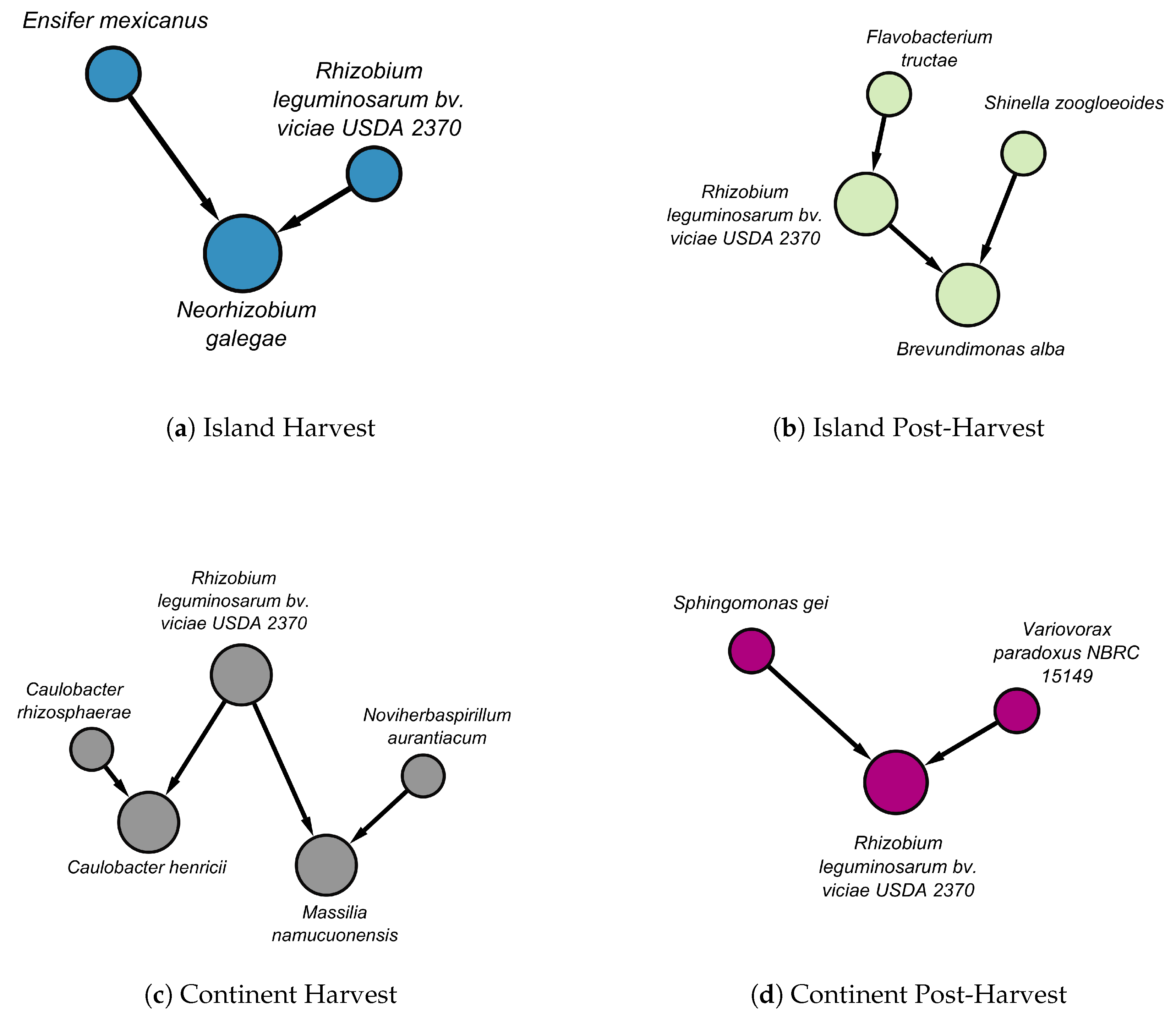
We identified not only local structures with matching edges but also local structures that differ between stages and terroirs. In Figure 5, the local structures of Rhizobium leguminosarum bv. viciae USDA 2370 are presented across stages and locations.
In island at the harvest stage, Rhizobium leguminosarum bv. viciae USDA 2370 and Ensifer mexicanus causally influenced Neorhizobium galegae (Figure 5(a)). In contrast, at the post-harvest stage, Rhizobium leguminosarum bv. viciae USDA 2370 received a directed edge from Flavobacterium tructae and, together with Shinella zoogloeoides, causally influenced Brevundimonas alba (Figure 5(b)).
In the continental terroir, Rhizobium leguminosarum bv. viciae USDA 2370 and Caulobacter rhizosphaerae causally influenced Caulobacter henricii. Additionally, they, together with Noviherbaspirillum aurantiacum, causally influenced Massilia namucuonensis (Figure 5(c)). At the post-harvest stage, Rhizobium leguminosarum bv. viciae USDA 2370 received directed influence from Sphingomonas gei and Variovorax paradoxus (Figure 5(d)).
We could not identify any matching edges between island and continental terroirs in the soil dataset. However, there are some relationships that differ between the island and continental terroirs. For example, in the island structure, Nitrospira japonica had an undirected edge with Nitrobacter winogradskyi, whereas in continental, Nitrospira japonica, together with Limisphaera ngamtamarikiensis, causally influenced Syntrophotalea carbinolica DSM (Supplementary Figure S5).
The number of reads for species in tubers from the island terroir and the continental terroir at harvest and post-harvest, as well as the number of reads for species in soil that were discussed or presented in figures, are provided in Supplementary Table S3.
4. Discussion
In this paper, we introduced the R package DAGMetrics, designed for evaluating and comparing DAGs. It provides an intuitive and easy-to-use framework for researchers seeking detailed insights into the structure of causal networks. The package’s visualization tools facilitated the exploration of DAGs, enabling to highlight key structural differences efficiently. Additionally, the ability to compare local structures allows to detect differences and similarities across different locations, time points and stages of a system. Another significant advantage of DAGMetrics is its ability to visualize not only the Markov blanket of a selected node but also to drill down further to display Markov blankets of multiple nodes. This feature enabled us to explore and compare multiple local structures simultaneously, allowing to focus on relationships of interest without displaying the full structure, which can be overwhelming, especially in high-dimensional datasets where the full structure may consist of hundreds of nodes. By providing this functionality, DAGMetrics makes it easier to analyze causal structures.
The package was then applied to two distinct metagenomic datasets, generated for the potato tuber and soil microbiome. DAGMetrics streamlined the comprehensive evaluation of outputs from various structure learning algorithms, aiding in the identification of the most appropriate DAGs for the downstream analysis. Additionally, it facilitated the description of the Markov blanket space of DAGs across different terroirs and stages. Finally, it enabled the identification of matching nodes and dissimilar Markov blankets in structures derived from different terroirs and stages.
From a model selection perspective, the comprehensive set of descriptive and comparative metrics provided by DAGMetrics allowed us to reflect on the desired characteristics of the selected DAG. The absence of a ground-truth DAG and the consequent inability to assess the accuracy of the learned structures remain a challenge. However, a detailed evaluation of the complexity, stability, and similarity of outputs of different structure learning algorithms with different scaling and transformation setups offered indirect indications of the robustness of the learned structures. Our analysis of two different datasets revealed consistent patterns in the behavior of structure learning algorithms. The PC algorithm with Spearman correlation produced balanced DAGs with moderate complexity and structural stability across various scaling and transformation techniques.
The description of the Markov blanket space provided insights into agronomic microbial abundance datasets. Despite challenges such as small sample sizes and high dimensionality, the datasets shared structural characteristics. These included many isolated nodes, moderately small Markov blankets (up to 7 nodes), and the existence of isolated substructures within the global structure.
The use of DAGs, as facilitated by the DAGMetrics package, has provided profound insights into the microbial dynamics within potato tubers at two physiological stages (at harvest and at post-harvest) from two diverse terroirs (island and continental). In particular, our results on the directed relationships between species such as Methylotenera mobilis and Methylotenera versatilis may suggest potential metabolic, genetic or ecological dependencies that are crucial for microbial stability and function. Both species belong to the family of Methylophilaceae, with the former being involved in the denitrification pathway, a capability that is integral to its role in nitrogen cycling, and the latter in methane metabolism, which is critical in the global carbon cycle and methane biotransformation [32,33]. Furthermore, these species can be found in similar environments, probably sharing some ecological niches, suggesting similarities in their metabolic capabilities and environmental adaptations which allows them to thrive in similar methylamine-rich environments [34]. Therefore, these interactions or associations make Methylotenera mobilis and Methylotenera versatilis critical, especially in environments where nutrient uptake and carbon cycling need to be stimulated [35]. Moreover, the persistent relationships across different stages and regions, such as those between Devosia psychrophila and Devosia submarina, highlight the robustness of microbial associations that potentially underpin critical processes such as decomposition and nutrient cycling, supporting the contribution of intricate microbial associations to the multifunctionality of agricultural ecosystems [36]. Although both species belong to the same genus, Devosia, they can be found in distinct environmental habitats, with Devosia psychrophile being adapted to cold environments, and Devosia submarina to marine ecosystems (deep sea sediments). In our study, these species were more abundant at the island terroir, suggesting sophisticated genetic and metabolic adaptations that enable them to thrive in their habitat. By further exploring the matching edges for both island and continental terroirs obtained from the DAGMetrics package, the complex and dynamic nature of microbial communities of potato tubers can be further unraveled, providing insights into the potential of regulating ecosystem functions by manipulating healthy microbial interactions.
These findings highlight the ability of DAGMetrics to reveal meaningful structural relationships within complex microbial datasets, demonstrating its potential as a valuable tool for causal discovery in agronomic research and beyond. By providing a broad range of descriptive and comparative metrics along with intuitive visualization capabilities, DAGMetrics enables a systematic evaluation of both global and local structures. The package facilitates the identification of structural similarities and differences across different conditions. Moreover, its ability to compare DAGs across multiple datasets, track structural changes, and highlight matching connections makes it a powerful resource for researchers.
Supplementary Materials
The following supporting information can be downloaded at the website of this paper posted on Preprints.org.
Author Contributions
Conceptualization, P.A. and T.M.; methodology, P.A. and T.M.; software, P.A.; validation, I.M. and T.M.; formal analysis, P.A.; investigation, T.M., M.G. and I.M.; resources, I.M. and I.X.; data curation, P.A. and I.M.; writing—original draft preparation, P.A. and I.M.; writing—review and editing, T.M., M.G., I.M., and A.X.; visualization, P.A.; supervision, T.M.; project administration, T.M.; funding acquisition, T.M. All authors have read and agreed to the published version of the manuscript.
Funding
This research received no external funding
Institutional Review Board Statement
Not applicable
Informed Consent Statement
Not applicable
Data Availability Statement
Raw data used in this study were obtained from the National Centre for Biotechnology Information (NCBI) Sequence Read Archive (SRA). The tuber dataset is available under the BioProject accession number PRJNA854325, and the soil dataset is available under the BioProject accession number PRJNA970975. These datasets can be accessed through the NCBI SRA database.
Conflicts of Interest
The authors declare no conflicts of interest.
References
- Sadeghi, A.; Gopal, A.; Fesanghary, M. Causal Discovery in Financial Markets: A Framework for Nonstationary Time-Series Data. arXiv 2023, arXiv:2312.17375. [Google Scholar] [CrossRef]
- Addo, P.M.; Manibialoa, C.; McIsaac, F. Exploring nonlinearity on the CO2 emissions, economic production and energy use nexus: a causal discovery approach. Energy Reports 2021, 7, 6196–6204. [Google Scholar] [CrossRef]
- Ebert-Uphoff, I.; Deng, Y. Causal discovery for climate research using graphical models. Journal of Climate 2012, 25, 5648–5665. [Google Scholar] [CrossRef]
- Agrahari, R.; Foroushani, A.; Docking, T.R.; Chang, L.; Duns, G.; Hudoba, M.; Karsan, A.; Zare, H. Applications of Bayesian network models in predicting types of hematological malignancies. Scientific reports 2018, 8, 6951. [Google Scholar] [CrossRef]
- Friedman, N.; Linial, M.; Nachman, I.; Pe’er, D. Using Bayesian networks to analyze expression data. In Proceedings of the Proceedings of the fourth annual international conference on Computational molecular biology; 2023; pp. 127–135. [Google Scholar]
- Foroushani, A.; Agrahari, R.; Docking, R.; Chang, L.; Duns, G.; Hudoba, M.; Karsan, A.; Zare, H. Large-scale gene network analysis reveals the significance of extracellular matrix pathway and homeobox genes in acute myeloid leukemia: an introduction to the Pigengene package and its applications. BMC medical genomics 2017, 10, 1–15. [Google Scholar] [CrossRef] [PubMed]
- Zhang, B.; Gaiteri, C.; Bodea, L.G.; Wang, Z.; McElwee, J.; Podtelezhnikov, A.A.; Zhang, C.; Xie, T.; Tran, L.; Dobrin, R.; et al. Integrated systems approach identifies genetic nodes and networks in late-onset Alzheimer’s disease. Cell 2013, 153, 707–720. [Google Scholar] [CrossRef]
- Ganopoulou, M.; Michailidis, M.; Angelis, L.; Ganopoulos, I.; Molassiotis, A.; Xanthopoulou, A.; Moysiadis, T. Could Causal Discovery in Proteogenomics Assist in Understanding Gene–Protein Relations? A Perennial Fruit Tree Case Study Using Sweet Cherry as a Model. Cells 2021, 11, 92. [Google Scholar] [CrossRef]
- Skodra, C.; Michailidis, M.; Moysiadis, T.; Stamatakis, G.; Ganopoulou, M.; Adamakis, I.D.S.; Angelis, L.; Ganopoulos, I.; Tanou, G.; Samiotaki, M.; et al. Disclosing the molecular basis of salinity priming in olive trees using proteogenomic model discovery. Plant Physiology 2023, 191, 1913–1933. [Google Scholar] [CrossRef]
- Boutsika, A.; Michailidis, M.; Ganopoulou, M.; Dalakouras, A.; Skodra, C.; Xanthopoulou, A.; Stamatakis, G.; Samiotaki, M.; Tanou, G.; Moysiadis, T.; et al. A wide foodomics approach coupled with metagenomics elucidates the environmental signature of potatoes. Iscience 2023, 26. [Google Scholar] [CrossRef]
- Brouillard, P.; Squires, C.; Wahl, J.; Kording, K.P.; Sachs, K.; Drouin, A.; Sridhar, D. The Landscape of Causal Discovery Data: Grounding Causal Discovery in Real-World Applications. arXiv 2024, arXiv:2412.01953. [Google Scholar]
- Spirtes, P.; Glymour, C.; Scheines, R. Causation, prediction, and search; MIT press, 2001. [Google Scholar]
- Pearl, J. Probabilistic Reasoning in Intelligent Systems: Networks of Plausible Inference; Morgan Kaufmann, 1988. [Google Scholar]
- Bouckaert, R.R. Bayesian belief networks: from construction to inference. PhD thesis, 1995. [Google Scholar]
- Tsamardinos, I.; Brown, L.E.; Aliferis, C.F. The max-min hill-climbing Bayesian network structure learning algorithm. Machine learning 2006, 65, 31–78. [Google Scholar]
- Scutari, M.; Graafland, C.E.; Gutiérrez, J.M. Who learns better Bayesian network structures: Accuracy and speed of structure learning algorithms. International Journal of Approximate Reasoning 2019, 115, 235–253. [Google Scholar]
- Constantinou, A.C.; Liu, Y.; Chobtham, K.; Guo, Z.; Kitson, N.K. Large-scale empirical validation of Bayesian Network structure learning algorithms with noisy data. International Journal of Approximate Reasoning 2021, 131, 151–188. [Google Scholar]
- Zheng, X.; Aragam, B.; Ravikumar, P.K.; Xing, E.P. Dags with no tears: Continuous optimization for structure learning. Advances in neural information processing systems 2018, 31. [Google Scholar]
- Fang, Z.; Zhu, S.; Zhang, J.; Liu, Y.; Chen, Z.; He, Y. On low-rank directed acyclic graphs and causal structure learning. IEEE Transactions on Neural Networks and Learning Systems 2023, 35, 4924–4937. [Google Scholar] [CrossRef]
- Ng, I.; Ghassami, A.; Zhang, K. On the role of sparsity and dag constraints for learning linear dags. Advances in Neural Information Processing Systems 2020, 33, 17943–17954. [Google Scholar]
- Huang, B.; Zhang, K.; Zhang, J.; Ramsey, J.; Sanchez-Romero, R.; Glymour, C.; Schölkopf, B. Causal discovery from heterogeneous/nonstationary data. Journal of Machine Learning Research 2020, 21, 1–53. [Google Scholar]
- Maeda, T.N.; Shimizu, S. RCD: Repetitive causal discovery of linear non-Gaussian acyclic models with latent confounders. In Proceedings of the International Conference on Artificial Intelligence and Statistics. PMLR; 2020; pp. 735–745. [Google Scholar]
- Maeda, T.N.; Shimizu, S. Causal additive models with unobserved variables. In Proceedings of the Uncertainty in Artificial Intelligence. PMLR; 2021; pp. 97–106. [Google Scholar]
- Shimizu, S.; Hoyer, P.O.; Hyvärinen, A.; Kerminen, A.; Jordan, M. A linear non-Gaussian acyclic model for causal discovery. Journal of Machine Learning Research 2006, 7. [Google Scholar]
- Boutsika, A.; Xanthopoulou, A.; Tanou, G.; Zacharatou, M.E.; Vernikos, M.; Nianiou-Obeidat, I.; Ganopoulos, I.; Mellidou, I. A microbiome survey of contrasting potato terroirs using 16S rRNA long-read sequencing. Plant and Soil 2024, 1–8. [Google Scholar]
- Kalisch, M.; Mächler, M.; Colombo, D.; Maathuis, M.H.; Bühlmann, P. Causal inference using graphical models with the R package pcalg. Journal of statistical software 2012, 47, 1–26. [Google Scholar] [CrossRef]
- Tsamardinos, I.; Aliferis, C.F.; Statnikov, A.R.; Statnikov, E. Algorithms for large scale Markov blanket discovery. In Proceedings of the FLAIRS, Vol. 2; 2003; pp. 376–81. [Google Scholar]
- Scutari, M. Learning Bayesian networks with the bnlearn R package. arXiv 2009, arXiv:0908.3817. [Google Scholar]
- Foroushani, A.; Agrahari, R.; Docking, R.; Chang, L.; Duns, G.; Hudoba, M.; Karsan, A.; Zare, H. Large-scale gene network analysis reveals the significance of extracellular matrix pathway and homeobox genes in acute myeloid leukemia: an introduction to the Pigengene package and its applications. BMC medical genomics 2017, 10, 1–15. [Google Scholar]
- Agrahari, R.; Foroushani, A.; Docking, T.R.; Chang, L.; Duns, G.; Hudoba, M.; Karsan, A.; Zare, H. Applications of Bayesian network models in predicting types of hematological malignancies. Scientific reports 2018, 8, 6951. [Google Scholar]
- Shannon, P.; Markiel, A.; Ozier, O.; Baliga, N.S.; Wang, J.T.; Ramage, D.; Amin, N.; Schwikowski, B.; Ideker, T. Cytoscape: a software environment for integrated models of biomolecular interaction networks. Genome research 2003, 13, 2498–2504. [Google Scholar]
- Kalyuzhnaya, M.G.; Beck, D.A.; Vorobev, A.; Smalley, N.; Kunkel, D.D.; Lidstrom, M.E.; Chistoserdova, L. Novel methylotrophic isolates from lake sediment, description of Methylotenera versatilis sp. nov. and emended description of the genus Methylotenera. International journal of systematic and evolutionary microbiology 2012, 62, 106–111. [Google Scholar]
- Mustakhimov, I.; Kalyuzhnaya, M.G.; Lidstrom, M.E.; Chistoserdova, L. Insights into denitrification in Methylotenera mobilis from denitrification pathway and methanol metabolism mutants. Journal of bacteriology 2013, 195, 2207–2211. [Google Scholar] [CrossRef] [PubMed]
- Salcher, M.M.; Schaefle, D.; Kaspar, M.; Neuenschwander, S.M.; Ghai, R. Evolution in action: habitat transition from sediment to the pelagial leads to genome streamlining in Methylophilaceae. The ISME journal 2019, 13, 2764–2777. [Google Scholar]
- Bulgarelli, D.; Rott, M.; Schlaeppi, K.; Ver Loren van Themaat, E.; Ahmadinejad, N.; Assenza, F.; Rauf, P.; Huettel, B.; Reinhardt, R.; Schmelzer, E.; et al. Revealing structure and assembly cues for Arabidopsis root-inhabiting bacterial microbiota. Nature 2012, 488, 91–95. [Google Scholar]
- Li, K.; Chen, A.; Sheng, R.; Hou, H.; Zhu, B.; Wei, W.; Zhang, W. Long-term chemical and organic fertilization induces distinct variations of microbial associations but unanimous elevation of soil multifunctionality. Science of The Total Environment 2024, 172862. [Google Scholar]
Figure 1.
Normalised number of edges, normalised number of colliders and normalised number of isolated nodes for island (haverst and post-harvest) and continental (harvest and post-harvest) terroirs accross models in the tuber dataset. On the x-axis are the models.
Figure 1.
Normalised number of edges, normalised number of colliders and normalised number of isolated nodes for island (haverst and post-harvest) and continental (harvest and post-harvest) terroirs accross models in the tuber dataset. On the x-axis are the models.
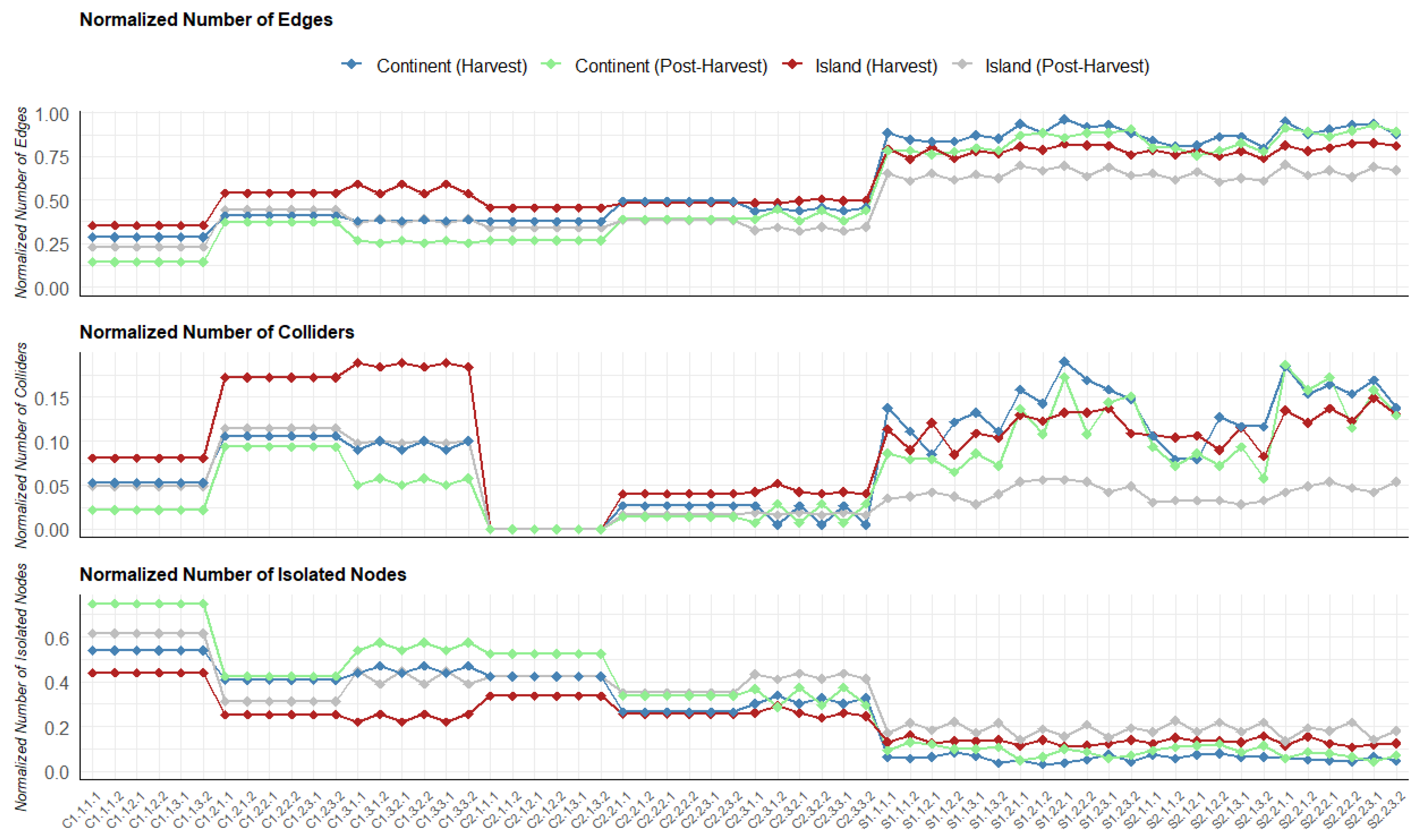
Figure 2.
This plot illustrates the similarity between the outputs of different structure learning algorithms, using the F1 score as a metric. It corresponds to the tuber dataset in island terroir at harvest stage.
Figure 2.
This plot illustrates the similarity between the outputs of different structure learning algorithms, using the F1 score as a metric. It corresponds to the tuber dataset in island terroir at harvest stage.
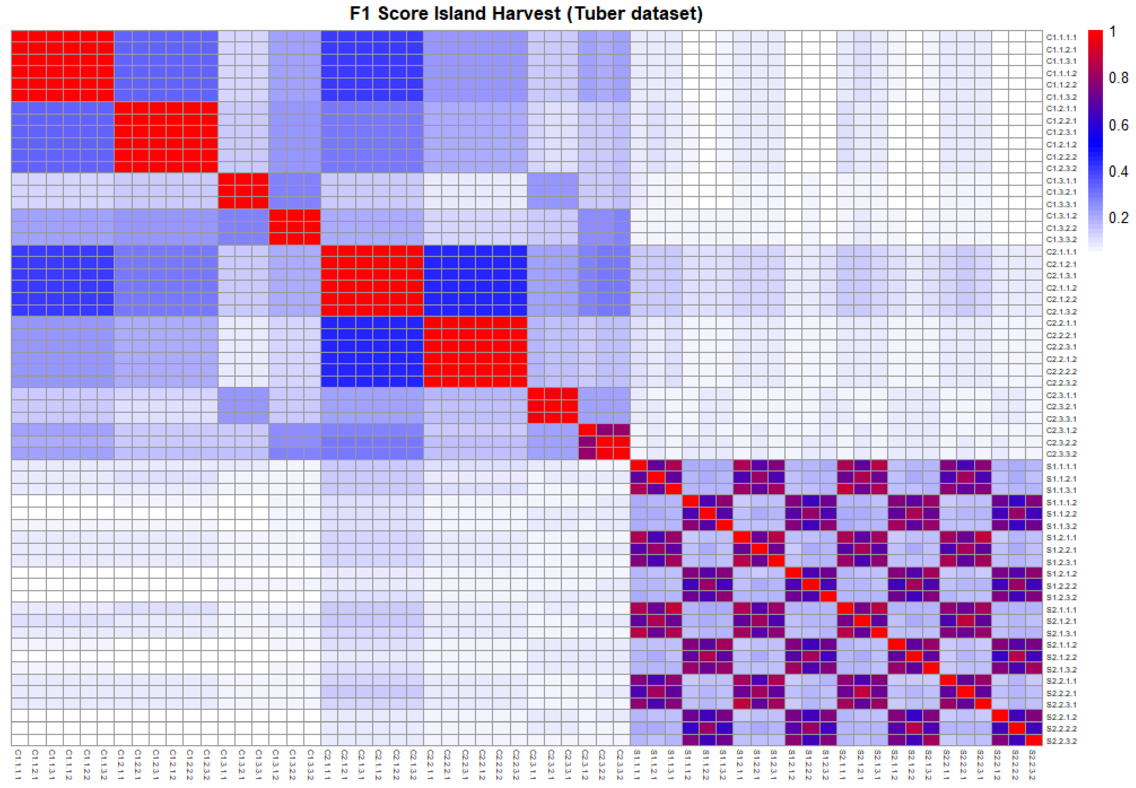
Figure 3.
This plot illustrates the distribution of Markov blankets in the tuber dataset, with horizontal panels representing different terroirs and stages and vertical panels corresponding to different metrics. The frequency of Markov blankets is displayed on the y-axis, while the x-axis represents the values of each metric. For example, the top-left panel shows the distribution of the number of colliders across Markov blankets in the continental harvest DAG. It indicates that over 100 Markov blankets had no colliders, more than 50 Markov blankets contained one collider, and a few Markov blankets had two colliders in their structure.
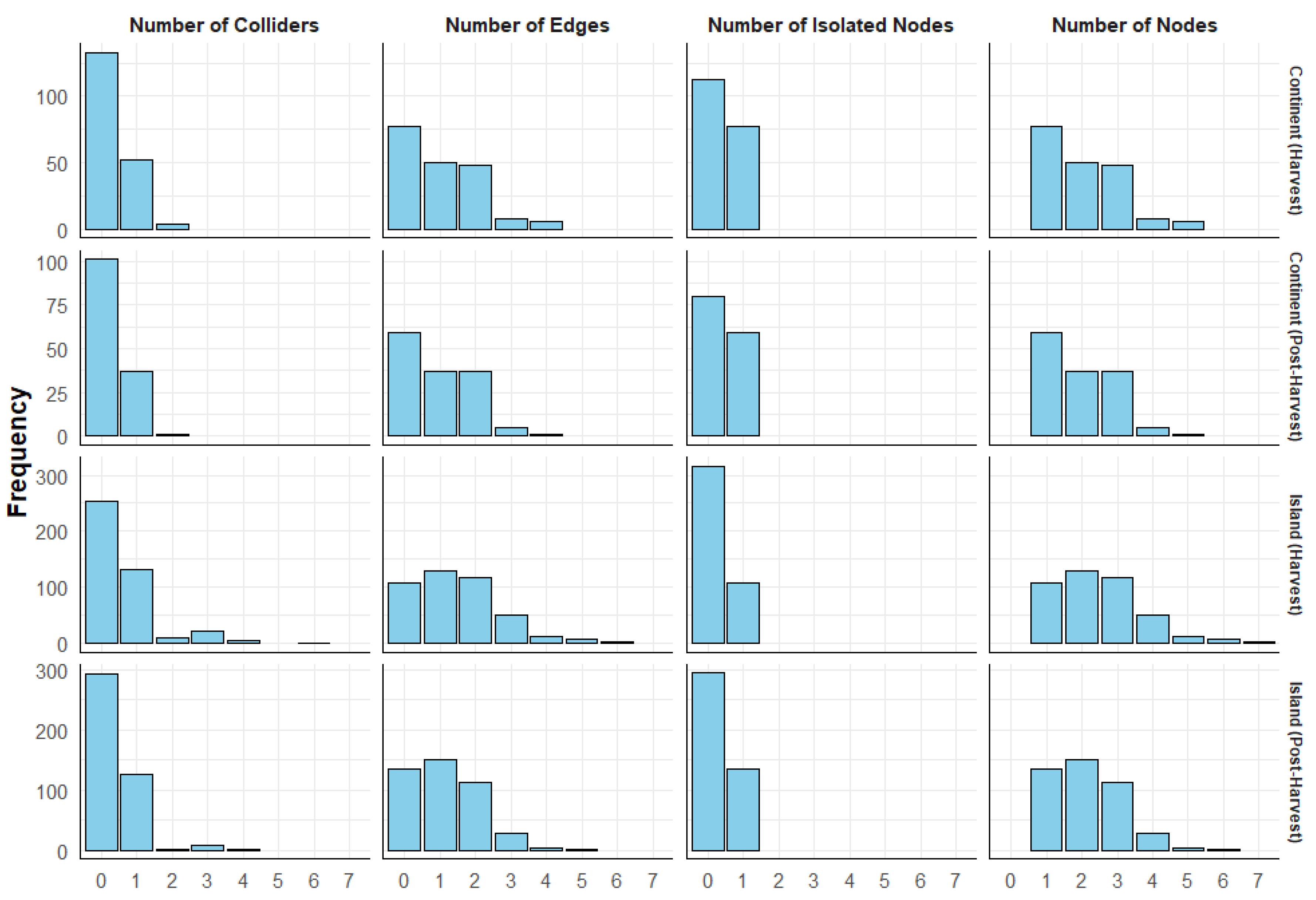
Figure 4.
The figure illustrates matching edges between DAGs across different terroirs and stages. (a) Nodes in island harvest are shown in blue. (b) Nodes in island post-harvest are in green. (c) Nodes in continental harvest are in gray. (d) Nodes in continental post-harvest are in purple. The edges in each panel are color-coded to indicate whether they match across different terroirs or stages. Black edges signify no match with any edge in another terroir or stage. Blue edges indicate a match with the island harvest DAG, green edges correspond to matches with the island post-harvest DAG, gray edges represent matches with the continental harvest DAG, and purple edges indicate matches with the continental post-harvest DAG. For example, in (b), a purple edge from Rhodoligotrophos appendicifer to Bartonella rochalimae indicates that a corresponding edge can be found in a DAG with purple nodes (d). Directed edges represent causal influence, whereas undirected edges denote uncertainty in the direction of influence.
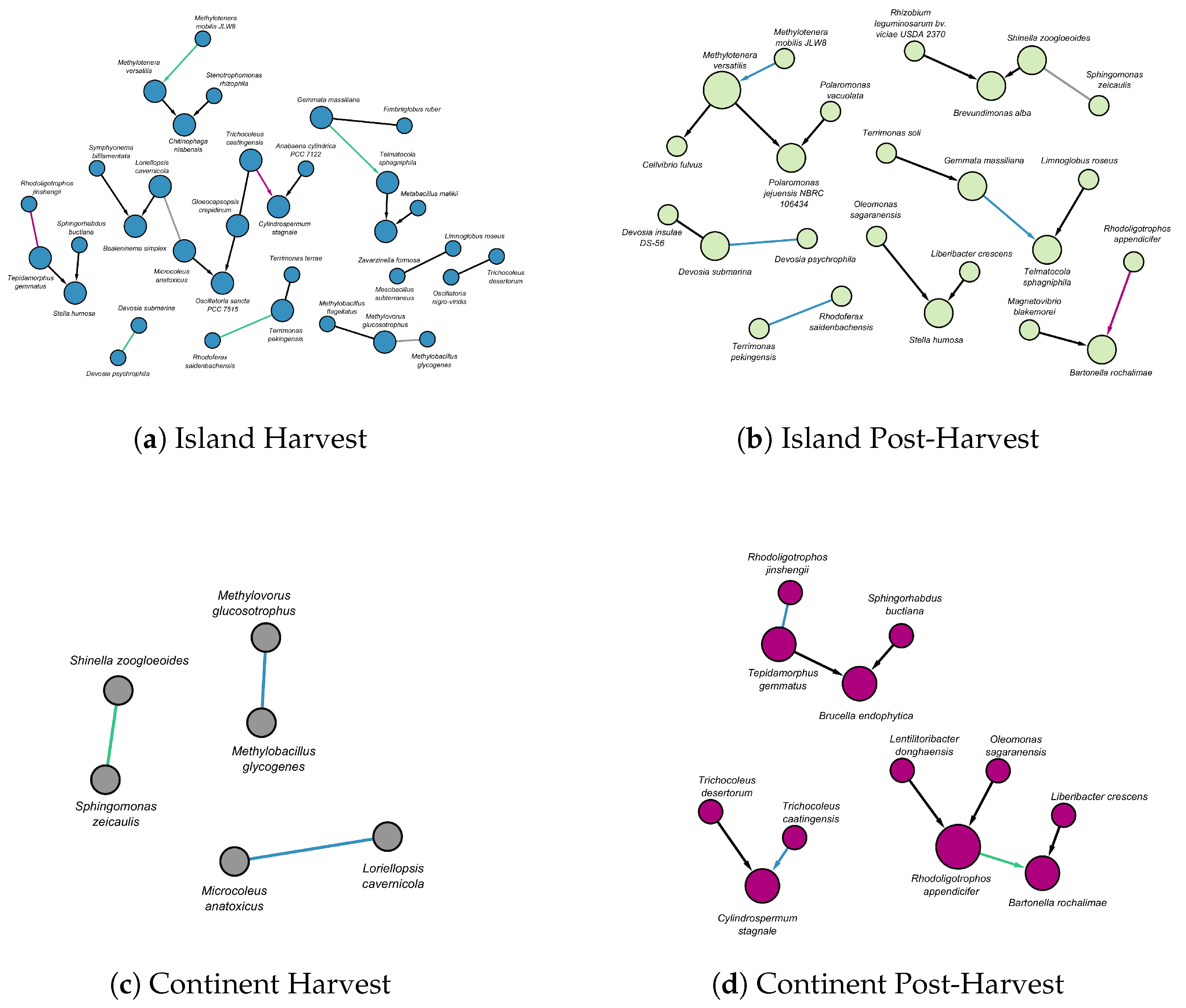
Figure 5.
The figure represents Markov blankets of Rhizobium leguminosarum bv. viciae USDA 2370 across different terroirs and stages in the tuber dataset (a) Nodes in the island at harvest are in blue color. (b) Nodes in the island at post-harvest are in green color. (c) Nodes in the continental terroir at harvest are in grey color. (d) Nodes in the continental terroir at harvest are in purple color. Edges in the panels have different color. Black color indicates that it does not match with any edge in different terroir or stage. Directed edges represent causal influence and undirected edges represent uncertatinty of the direction of influence.
Disclaimer/Publisher’s Note: The statements, opinions and data contained in all publications are solely those of the individual author(s) and contributor(s) and not of MDPI and/or the editor(s). MDPI and/or the editor(s) disclaim responsibility for any injury to people or property resulting from any ideas, methods, instructions or products referred to in the content. |
© 2025 by the authors. Licensee MDPI, Basel, Switzerland. This article is an open access article distributed under the terms and conditions of the Creative Commons Attribution (CC BY) license (http://creativecommons.org/licenses/by/4.0/).
Copyright: This open access article is published under a Creative Commons CC BY 4.0 license, which permit the free download, distribution, and reuse, provided that the author and preprint are cited in any reuse.


