Submitted:
01 March 2025
Posted:
12 March 2025
You are already at the latest version
Abstract
Liver cancer remains a critical global health challenge, with accurate segmentation of tumors in CT scans being vital for diagnosis. While deep learning models like U-Net and Vision Transformers offer promising results, their high computational demands hinder deployment on resource-constrained edge devices. This study introduces an optimized Swin-UNet model for efficient liver tumor segmentation, leveraging a Search and Rescue (SAR) algorithm to balance model size and accuracy. Key innovations include a quadratic penalty-based objective function for joint optimization of AUC and model compactness and a focal AUC loss to address class imbalance. Evaluated across three datasets (3DIRCADb, LiTS, MSD), the proposed SAR-Swin-UNet achieves superior performance, with Dice scores of 94.78%, 89.06% and 88.95%, respectively, while reducing the model size by up to 80.3% compared to unoptimized counterpart. The approach enables real-time, energy-efficient segmentation on edge devices like Jetson Nano, addressing challenges of data security and computational costs. Results demonstrate significant improvements over state-of-the-art methods with a minimum Volume Overlap Error of (1.73%) in MSD dataset and Relative Volume Difference of (0.23%) in 3DIRCADb dataset, highlighting its clinical applicability for precise, low-resource settings. This work bridges the gap between high-accuracy segmentation and practical deployment in under-resourced healthcare environments.
Keywords:
Liver tumor segmentation
; Swin-UNet
; Search and Rescue algorithm
; Memory-Constrained Devices
1. Introduction
Liver cancer (LC) is a significant global health concern, ranking as one of the most commonly diagnosed cancers and the leading cause of cancer-related deaths. Recent global statistics position liver cancer as the sixth most prevalent cancer, following breast, lung, colorectal, prostate and gastric cancers and as the third leading cause of cancer mortality. In 2020, approximately 905,700 new cases and 830,200 deaths from LC occurred worldwide [1]. Hepatocellular carcinoma (HCC), the most common form of LC, accounts for nearly 90% of all cases [2]. Various imaging techniques such as ultrasound, elastography, MRI and CT scans detect LC, with CT scans providing detailed images of internal structures [3]. However, CT imaging encounters challenges in detecting and diagnosing liver abnormalities accurately. The liver’s varying sizes and shapes cause incorrect segmentation due to the similarity in intensity between tumors and surrounding tissues and unclear lesion boundaries. These factors make manual annotation by radiologists time-intensive and error-prone, leading to inconsistencies in diagnosis.
Medical image segmentation achieves progress in improving cancer diagnosis accuracy and computer-aided diagnosis (CAD) systems assist in the detection, classification, and segmentation of tumours on medical images, reduces radiologists’ workload and increases diagnostic consistency [4,5,6,7,8,9]. Deep learning models, particularly Convolutional Neural Networks (CNNs), automate this segmentation process. Fully Convolutional Networks (FCNs) and U-Net architectures also segment liver tumors by performing pixel-wise classification [10]. Despite their high accuracy compared to manual segmentation, such models require significant computational resources, complicating deployment on edge devices with limited processing power and memory. Large servers are necessary to run these models, causing issues like bandwidth usage, data security, high server costs and substantial carbon footprints due to increased energy consumption compared to resource-constrained embedded systems. Thus, resource-efficient models are needed for accurate liver tumor segmentation on constrained devices.
Liver tumor segmentation techniques include traditional image processing, supervised learning and unsupervised learning methods. Traditional image processing techniques, such as thresholding [11], Canny edge detection [12] and watershed segmentation [13], rely on edge detection and intensity thresholding to differentiate tumor regions from normal tissue. Thresholding separates objects based on intensity, while watershed segmentation uses gradients to define boundaries. These methods struggle with the complexity of medical images, where tumors exhibit irregular shapes, variable sizes and similar intensity values to surrounding tissues, leading to errors [14]. Additionally, traditional methods often require manual or semi-automatic intervention, increasing dependency on expert input for accuracy.
Unsupervised learning methods address limitations in traditional techniques by segmenting tumors without labeled data. Notable methods include clustering-based techniques and edge-based algorithms. For instance, Al-Kofahi et al. [15] introduced a multi-scale Laplacian of Gaussian (LoG) filter for histopathology images to detect nuclei of varying sizes. Kong et al. [16] developed a generalized LoG filter (gLoG) to detect elliptical nuclei in histopathology images, which can apply to LC segmentation in CT scans. Despite their potential, unsupervised methods require careful parameter tuning, are sensitive to noise and struggle to define tumor boundaries with low contrast [17]. Combining unsupervised techniques with region-based methods, such as Active Contour Models (ACM) [18] and marker-based watershed transforms [19], improves segmentation accuracy but remains computationally expensive and less generalizable across datasets.
CNNs, FCNs and U-Net variants dominate the field of medical image analysis due to their ability to learn hierarchical features from complex medical images. For instance, Saha Roy et al. [20] proposed an automated model that utilizes Mask R-CNN followed by Maximally Stable Extremal Regions (MSER) for tumor identification, enabling multi-class tumor classification. Chen et al. [21] proposed MS-FANet, a multi-scale feature attention network that performs liver tumor segmentation through multi-scale attention mechanisms which boost segmentation capabilities while capturing both global and local context. Lakshmi et al. [22] designed the Adaptive SegUnet++ (ASUnet++) framework and optimized it with the Enhanced Lemurs Optimizer (ELO) for tumor segmentation and classification. The authors’ model tackles traditional machine learning hurdles including slow training times and gradient explosion issues as well as overfitting using both residual connections and multiscale approaches. Reyad et al. [23] proposed an architecture optimization framework for hybrid deep residual networks in liver tumor segmentation, utilizing a Genetic Algorithm (GA) to improve segmentation accuracy and model efficiency. Di et al. [24] developed a framework for automatic liver tumor segmentation which integrates 3D U-Net architecture with hierarchical superpixels and SVM-based classification, achieving robust performance on noisy and low-contrast CT images. Liu et al. [25] introduced PA-Net, a phase attention network that fuses venous and arterial phase features of CT images for liver tumor segmentation, effectively leveraging phase-specific information to enhance segmentation performance. CNN-based approaches have shown powerful representation abilities together with resilience to different image appearances. However, CNNs are inherently limited in modeling long-range dependencies, which can lead to suboptimal segmentation outcomes. Specifically, the localized receptive fields of convolutional operations restrict the network’s focus to local context rather than global context [26].
Transformers which were initially created for sequence-to-sequence prediction tasks now play a primary role in computer vision tasks. Transformers demonstrate outstanding performance across multiple computer vision tasks including image classification [27], object detection [28], semantic segmentation [29] and generative tasks like text-to-image synthesis [25]. Transformers achieve success because their self-attention mechanism provides large receptive fields and long-range dependency capturing abilities. Medical image segmentation tasks have seen multiple proposals for hybrid methods that integrate both CNNs and Transformers. For instance, Balasubramanian et al. [30] proposed APESTNet, a Mask R-CNN-based Enhanced Swin Transformer Network for tumor segmentation and classification. This method combines the strengths of Mask R-CNN with the attention mechanisms of the Swin Transformer to improve segmentation accuracy. Chen et al. [31] introduced TransUNet, a cascaded architecture that integrates CNN and Transformer modules to enhance segmentation performance. Ni et al. [32] presented DA-Tran, a domain-adaptive transformer network for multiphase liver tumor segmentation. DA-Tran leverages domain adaptation techniques to effectively integrate multiphase CT images, improving segmentation accuracy and robustness across varying imaging conditions.
Despite their accuracy, existing models require substantial memory and computational power, which are unsuitable for edge devices like Jetson Nano. These models typically operate on server systems, demanding sensitive patient data transfer over the Internet, raising privacy and security concerns. High server energy consumption limits feasibility in resource-constrained settings. Optimizing segmentation models to reduce size and power consumption while maintaining accuracy enables deployment on edge devices for real-time, secure and energy-efficient tumor segmentation.
This study proposes a novel approach to optimize the Swin-UNet model for efficient liver cancer segmentation on edge devices, balancing model size and Area Under the Curve (AUC). Contributions include:
- Model Size Optimization: The discrete design space of Swin-UNet achieves a balance between model size and accuracy, enabling deployment on memory-constrained devices like Jetson Nano.
- Quadratic Penalty Objective Function: A quadratic penalty-based objective function balances model size and AUC, encouraging compact, accurate models.
- Search and Rescue Algorithm: The Search and Rescue algorithm identifies optimal configurations, yielding an optimized model termed SAR-Swin-UNet.
- Focal AUC Loss Function: The Focal AUC loss function addresses class imbalance during training, enhancing the model’s ability to segment minority class pixels.
This approach facilitates accurate tumor segmentation on edge devices, ensuring real-time analysis with data security and energy efficiency.
2. Preliminary Knowledge
This section discusses key architectures used in computer vision, specifically Transformer models for feature extraction and U-Net for segmentation. These architectures serve different purposes: Transformer models excel at feature extraction, especially for tasks like image classification, while U-Net is optimized for image segmentation tasks. A detailed discussion of both architectures is provided, along with key equations and variable explanations.
2.1. The Transformer Model
The Transformer architecture, first introduced by Vaswani et al. [33], revolutionized sequence-based models by replacing the recurrent mechanisms with a self-attention mechanism. This shift enabled parallel processing of input data, significantly improving computational efficiency. The central operation in the Transformer is the scaled dot-product attention, which can be expressed as:
where, Q, K and V are matrices representing the query, key and value vectors, respectively. The dimensions of these matrices are as follows:
where n is the sequence length (number of tokens), is the dimensionality of the query and key vectors and is the dimensionality of the value vectors. The attention mechanism computes a sum of the value vectors, where the weights are determined by the similarity between the query and key vectors. This self-attention mechanism is applied to model dependencies across the entire sequence. In the context of image-based tasks, this model is typically applied after embedding image patches into tokens, as in the Vision Transformer (ViT), which we discuss in the next subsection.
2.2. The Vision Transformer (ViT)
The Vision Transformer (ViT) [34], adapts the Transformer architecture to image classification tasks by treating image patches as tokens. Given an input image , where H is the height, W is the width and C is the number of channels, the image is divided into non-overlapping patches of size . These patches are then flattened and projected into an embedding space. The projection of patch can be formulated as:
where is the embedding matrix, is the embedding bias and is the number of patches. Each embedded patch is treated as a token and passed through the Transformer layers. The model utilizes multi-head self-attention and feed-forward networks, as described previously. However, ViT relies heavily on large datasets for training and performs well when pre-trained on large-scale data and fine-tuned on specific tasks. The advantage of ViT lies in its ability to capture global dependencies across image patches, which is a limitation in conventional CNNs that rely on localized receptive fields. However, ViT requires significant computational resources and large datasets to perform optimally.
2.3. The Swin Transformer
The Swin Transformer [35] presents a modification to the traditional Vision Transformer (ViT) architecture by addressing the challenges associated with computational complexity when working with high-resolution images. Unlike ViT, which applies global self-attention across all image patches, the Swin Transformer utilizes a local window-based attention mechanism. This local attention significantly reduces the computational burden, making the Swin Transformer more scalable for large images. Furthermore, it incorporates a hierarchical structure that progressively increases the receptive field, allowing the model to capture both local and global features at different levels.
In the Swin Transformer, the attention mechanism is applied within non-overlapping local windows. The self-attention within each window is computed independently and the output of each window is aggregated. The key innovation, however, is the introduction of a shifting window mechanism, which is applied to successive layers of the transformer. This shift allows the model to capture long-range dependencies between neighboring regions, which would otherwise be difficult to achieve with strictly local attention. The attention mechanism with the shifted window is expressed as follows:
where, Q, K and V are the query, key and value matrices, respectively and is the dimensionality of the key vectors. The term represents the shift between windows that occurs at successive layers of the model. This shift is critical for allowing information to propagate between neighboring windows, ensuring that global dependencies can still be captured, despite the local nature of the attention in the first few layers. The introduction of the shift operation helps the Swin Transformer overcome the limitations of purely local attention, providing the benefits of both local and global feature learning.
To clarify the role of each variable in the equation: - : The query matrix, where n is the number of patches in the window and is the dimensionality of the query vector. - : The key matrix, which has the same shape as the query matrix. - : The value matrix, used to compute the sum of the values based on the attention scores. - : The shift term introduced between successive layers to enable the exchange of information between neighboring windows.
Unlike the original Transformer where attention is computed globally across the entire image, the Swin Transformer confines attention within local windows at the early layers of the model, dramatically reducing computational complexity. The local-to-global attention mechanism is achieved by shifting the window between layers, gradually increasing the receptive field and allowing the model to capture long-range dependencies. This hierarchical design makes the Swin Transformer particularly well-suited for vision tasks such as image classification and object detection, where both fine-grained details and global context are important.
In contrast to the Vision Transformer, where the attention mechanism is applied globally across the entire input sequence (i.e., all patches in the image), the Swin Transformer introduces a more efficient mechanism by limiting attention to small, local windows. However, the shift in windows at each layer ensures that information is shared across windows, thus enabling the model to learn long-range dependencies. The computational complexity of the self-attention operation in the Swin Transformer is reduced to , where N is the number of patches and W is the window size, as opposed to the complexity in ViT, which computes attention globally for all image patches. This reduction in complexity allows Swin Transformer to scale to much larger images without sacrificing performance.
The key distinction between the attention mechanisms in ViT and Swin Transformer lies in the handling of attention: ViT computes attention globally, leading to high computational costs, while Swin Transformer limits attention to smaller local regions and uses shifting windows to propagate information across the image. This strategy makes Swin Transformer significantly more efficient and scalable for high-resolution images. Hence, the Swin Transformer improves on the Vision Transformer by using a local window-based self-attention mechanism combined with a hierarchical structure. This approach reduces computational complexity while still capturing both local and global dependencies, making it more efficient for vision tasks.
2.4. U-Net for Segmentation
U-Net, first introduced by Ronneberger et al. [36], is a convolutional neural network (CNN) architecture specifically designed for the task of semantic segmentation, with particular success in the field of medical imaging. The architecture follows a distinct encoder-decoder structure, augmented by skip connections, which allows the model to recover spatial information that might otherwise be lost during the downsampling process in the encoder section.
The encoder is composed of a series of convolutional operations, where the spatial resolution of the input image is progressively reduced, enabling the network to focus on increasingly abstract features. At each layer of the encoder, the feature map at layer l is computed as follows:
where, denotes the convolutional filter applied at layer l, * indicates the convolution operation, is the bias term and represents the activation function, typically ReLU. Through this process, the spatial resolution of the feature map is reduced, which increases the depth of the feature map, allowing the model to capture higher-level abstract features that represent the content of the input image.
In contrast, the decoder aims to reverse the downsampling performed by the encoder. This is achieved through the use of upsampling layers, often implemented as transposed convolutions, which progressively restore the spatial resolution of the feature map. The upsampling operation at decoder layer l can be represented as:
where, represents the transpose convolution filters and is the upsampled feature map. The skip connections between the corresponding layers of the encoder and decoder are particularly important, as they allow fine-grained spatial information to be transferred from the encoder to the decoder, preserving the precise localization of the segmentation boundaries. This aspect of U-Net ensures that the final segmentation mask is both accurate and spatially precise.
To produce the final output of the network, the feature map produced by the decoder is typically passed through an activation function. For multi-class segmentation tasks, a softmax activation is commonly applied, while for binary segmentation tasks, a sigmoid activation is used. The final segmentation mask is computed as follows:
In this equation, and are the final weights and biases and is the last feature map produced by the decoder. The architecture of U-Net, with its careful design of encoder-decoder structures and skip connections, is particularly well-suited for applications requiring precise, pixel-level segmentation, such as in medical imaging tasks.
When compared to Transformer-based models, such as the Vision Transformer (ViT) and the Swin Transformer, it becomes clear that U-Net serves a very different function. Transformer models are generally optimized for feature extraction tasks, particularly in the context of image classification, where the primary goal is to extract high-level semantic features and classify images based on these global contexts. While these models are highly effective for such tasks, their reliance on self-attention mechanisms and large datasets for training can make them computationally expensive. Additionally, they are less efficient when it comes to tasks that require pixel-level precision, such as segmentation.
In contrast, U-Net was specifically designed for segmentation tasks. The encoder-decoder structure with skip connections allows U-Net to capture both high-level features and fine-grained spatial details, making it particularly effective for segmentation tasks in medical imaging, where pixel-level accuracy is critical. U-Net’s ability to preserve fine-grained spatial information, which is often lost in deeper networks, makes it an ideal choice for these types of tasks.
Hence, Transformer models are better suited for tasks involving feature extraction and classification, especially when global context is a key consideration. On the other hand, U-Net excels in tasks that require fine-grained segmentation, where precise spatial localization is essential for accurate predictions.
3. Proposed Methodology
This section explains the methodology developed to optimize the Swin-UNet model for liver cancer segmentation, specifically targeting its deployment on memory-constrained edge devices. The approach consists of four primary components, each playing a critical role in ensuring that the model performs with high accuracy while adhering to the computational limitations inherent in edge devices.
The methodology integrates the Swin-UNet architecture, which combines the Swin Transformer and U-Net framework, offering a powerful solution for medical image segmentation, particularly for liver cancer. The Swin Transformer’s ability to capture both local and global features is crucial for accurate segmentation, but achieving peak performance requires optimization of the model’s hyperparameters. This is accomplished through the Search and Rescue (SAR) algorithm, which systematically explores and adjusts the hyperparameter space, minimizing an objective function that balances both model accuracy and size. Central to this approach is the formulation of an objective function that optimizes two key factors: the Area Under the Curve (AUC) for classification performance and the model size to ensure feasibility on memory-constrained edge devices. Additionally, the use of AUC focal loss enhances training, particularly for imbalanced datasets, by focusing on difficult-to-classify examples, such as challenging liver cancer lesions, thereby improving segmentation accuracy and robustness.
Each component of this methodology is supported by mathematical formulations that elucidate the underlying principles and mechanisms at play. These formulations are not merely theoretical; they provide the foundation for the practical implementation of the optimization process, demonstrating why the proposed approach is both effective and efficient. A block diagram, shown in Figure 1, illustrates the flow of the methodology, visually capturing the interactions between the various components.
The dataset used for training is divided into three distinct parts: a training set, a validation set and a test set. The SAR optimization algorithm is employed to fine-tune the hyperparameters, progressively reducing the objective function value. This iterative process ensures that the model’s accuracy increases while the size remains constrained. After the hyperparameters have been optimized, the final model is trained and the results are computed based on this optimized configuration. The next subsections will explore each of these components in greater detail, providing a deeper understanding of the methodology’s theoretical and practical foundations.
3.1. Swin-UNet and Hyperparameter Optimization
The Swin-UNet model integrates the hierarchical structure and shifted window attention mechanism of the Swin Transformer into the encoder-decoder framework of UNet as shown in the Figure 2. This subsection overviews the Swin-UNet architecture and details the hyperparameters that significantly impact model performance and memory efficiency.
3.1.1. Multi-Head Self-Attention (MHSA) in Swin-UNet
Swin-UNet employs a localized attention mechanism within non-overlapping windows, which differs from the global self-attention used in traditional Vision Transformers (ViTs). The attention mechanism for each window is computed as follows:
where, Q, K and V are the query, key and value matrices, respectively and is the dimensionality of the keys. This localized approach reduces the computational complexity compared to global attention mechanisms, making it more suitable for deployment on edge devices.
To facilitate spatial information exchange between windows, the Swin Transformer employs a shifted windowing mechanism, mathematically expressed as:
where, represents the offset applied to window positions. This mechanism allows the model to capture inter-window dependencies, enhancing the overall segmentation accuracy of liver tumors.
3.1.2. Hyperparameter Space and Constraints
The efficiency and performance of the Swin-UNet model are influenced by several key hyperparameters, each subject to specific constraints. Table 1 summarizes these hyperparameters along with their optimization ranges:
These hyperparameters control various aspects of the model, such as its depth, capacity and the size of the input data it processes. Optimizing these parameters within their specified ranges ensures a balance between the model’s segmentation accuracy and its memory footprint.
3.2. Search and Rescue (SAR) Algorithm
The Search and Rescue (SAR) algorithm [37], is a robust optimization method inspired by the processes involved in rescue missions. It has been successfully employed to solve complex optimization problems across various domains, especially where large, high-dimensional search spaces need to be explored efficiently. SAR’s strength lies in its ability to balance two crucial components: global exploration, which allows it to search broadly through the parameter space and local refinement, which focuses the search on the most promising regions. This dual approach makes SAR particularly effective for problems that require both exploration and fine-tuning, ensuring the identification of optimal or near-optimal solutions without falling into local minima.
In machine learning, hyperparameter optimization is a prime example of such a problem. Hyperparameter selection is critical to the performance of machine learning models, where improper tuning can lead to suboptimal results. In the case of algorithms such as neural networks, decision trees and support vector machines, the configurations of hyperparameters—such as learning rate, depth and regularization parameters—significantly influence model accuracy, training time and generalization capabilities. However, due to the high dimensionality of the hyperparameter search space and the computational cost of evaluating each configuration, hyperparameter optimization becomes a challenging task. SAR’s efficiency in navigating large search spaces, coupled with its ability to exploit promising areas while avoiding local minima, makes it an excellent candidate for optimizing hyperparameters in machine learning models. It enables adaptive refinement, allowing the model to converge towards optimal solutions while balancing the trade-offs between performance and computational efficiency.
In this study, SAR is applied for the first time to hyperparameter optimization in the context of medical image segmentation tasks. By employing SAR, we aim to optimize the configurations of a Swin-UNet architecture for liver tumor segmentation, which requires the careful tuning of parameters to achieve both high segmentation accuracy and computational efficiency.Figure 3 shows the overall block diagram of SAR-based hyperparameter optimization.
3.2.1. SAR Optimization Phases
SAR operates in three key phases: Initialization, Search and Rescue. These phases integrate both global search strategies and local refinement to ensure the algorithm explores the parameter space widely and then fine-tunes the promising regions. The following sections provide a detailed breakdown of each phase, followed by the mathematical formulations that guide the optimization process.
Initialization Phase:
The algorithm starts by generating an initial population of candidate solutions , where each solution represents a potential set of hyperparameters. These candidate solutions are randomly sampled within predefined bounds, which are set based on prior knowledge or expert intuition about the parameter space. The initialization phase plays a critical role in setting the starting point of the optimization and the quality of the initial candidates can significantly impact the subsequent search process.
The fitness of each candidate solution is evaluated using a fitness function that considers two key aspects: model performance (measured by AUC) and model size (which affects computational efficiency). The fitness function is formulated as follows:
where represents a set of hyperparameters for candidate solution i, is a scaling factor that controls the influence of model size and AUC denotes the area under the receiver operating characteristic (ROC) curve. This formulation ensures that the fitness function rewards configurations that achieve high accuracy while keeping the model size manageable.
Search Phase:
Once the initial population is generated and evaluated, the SAR algorithm enters the Search phase. During this phase, each candidate solution is assessed based on its fitness score and the algorithm iteratively updates the positions of the solutions. The goal is to explore the search space and identify regions that are most promising, based on the fitness function. The search process is carried out using the following formula for updating the positions of each candidate:
where is a learning rate parameter and refers to the solution with the highest fitness score among the neighboring solutions. By updating the position of each candidate solution iteratively, SAR ensures that the search is directed towards regions of the search space that hold the potential for better performance.
Rescue Phase:
After the Search phase, the algorithm proceeds to the Rescue phase, where further refinement of the solutions is performed. During this phase, the candidate solutions are adjusted based on their proximity to the best solutions found during the Search phase. The goal of the Rescue phase is to focus the search on the most promising regions, fine-tuning the hyperparameters in order to improve model performance. To adjust the candidate solutions, the algorithm uses two strategies. First, if a suitable neighboring solution is found, the candidate solution is updated by moving it toward the best-performing neighbor. The adjustment is calculated as given in Equation (10). If no suitable neighbors are found, the candidate solution is adjusted towards the globally best solution identified during the Search phase. The update for this adjustment is given by:
where and are scaling factors that control the magnitude of the adjustments. These strategies ensure that the algorithm refines the solutions towards the most optimal configurations while maintaining a balance between exploration and exploitation. The iterative process of the Rescue phase continues until the algorithm converges, yielding an optimal or near-optimal set of hyperparameters that balances both model performance (AUC) and model size, ensuring efficient training and accurate predictions.
3.3. AUC Focal Loss for Class Imbalance
Liver tumor segmentation tasks often involve significant class imbalance, where tumor pixels are underrepresented compared to healthy tissue pixels. To address this imbalance, the AUC focal loss is employed during the training phase, focusing the model’s learning on the minority class. This loss function modulates the contribution of easy and hard examples to the total loss, thereby prioritizing the harder-to-classify tumor pixels. The AUC focal loss is formulated as follows:
where controls the weighting of the positive (minority) class and adjusts the focus on difficult-to-classify examples. The parameters and are optimized within specific ranges, and , to ensure effective handling of class imbalance in liver tumor segmentation. The combination of SAR for hyperparameter optimization and AUC focal loss during training enables the development of a robust and efficient Swin-UNet model optimized for liver tumor segmentation, capable of delivering high-quality results even on memory-constrained edge devices.
By combining the SAR algorithm with the objective function and employing AUC focal loss during training, the resulting Swin-UNet model is optimized for efficient and accurate liver tumor segmentation on memory-constrained edge devices. The pseudo-code is given in Algorithm 1.
| Algorithm 1:Search and Rescue (SAR) Algorithm for Swin-UNet Optimization. |
|
3.4. Optimality Analysis of the Objective Function with SAR
The objective function used in this study is given by Equation (9). Where is a set of hyperparameters that includes both discrete and continuous variables. This function is designed to balance model accuracy (AUC) with model size, where is a positive constant that controls the trade-off. Given that includes a combination of discrete and continuous variables, the optimization process operates in a mixed space. Thus, traditional convexity concepts apply only to the continuous subspace.
Convexity in the Continuous Subspace:
For a fixed discrete setting of , consider the continuous component . The objective function within this continuous subspace can be simplified as:
where and .
The convexity analysis in this continuous domain reveals that the Hessian matrix H of this function is given by:
The determinant of this Hessian matrix is:
Since and , . However, since , the function is not strictly convex but exhibits convexity in a weaker sense. This suggests that the function has flat regions in the continuous domain, leading to multiple suboptimal solutions rather than a unique global optimum.
Optimality in the Discrete Space:
In the context of discrete variables, traditional convexity does not directly apply. However, the concept of piecewise convexity and discrete optimization can be leveraged. For the discrete components of , the objective function can be viewed as a set of piecewise convex functions:
where each represents the objective function in the continuous subspace for a fixed discrete setting j. Each function is convex, as previously proven.
Although the discrete space lacks a gradient, the SAR algorithm explores it by evaluating a finite set of configurations. SAR employs a combination of local search and global adjustment strategies to navigate this space, effectively finding a configuration that minimizes the objective function.
Suboptimality and Convergence with SAR:
SAR ensures that the search process converges to a suboptimal solution in the mixed space. Given that the continuous subspace is convex for fixed discrete settings, SAR optimizes locally in these regions as given by Equation (10). In cases where discrete changes are necessary, SAR adjusts the discrete variables, re-evaluating the objective function. This iterative process guarantees convergence to a suboptimal or near-optimal solution due to the following:
- Local Optimality in Continuous Subspace Each continuous optimization step finds a locally optimal solution within the convex region.
- Global Exploration in Discrete Space By systematically exploring different discrete configurations, SAR ensures broad coverage of the search space.
Thus, while strict convexity in the discrete space is not mathematically provable, the combination of convexity in the continuous space and SAR’s exploration mechanism ensures effective navigation towards at least a suboptimal point.
4. Results and Discussion
This section discusses the results and comparisons for the proposed scheme. It begins with an overview of the datasets and comparison metrics used to evaluate the scheme. Following this, the optimal hyperparameters are presented, along with an analysis of the model’s performance on various datasets. Finally, the section compares the proposed scheme with recently introduced schemes that have used the same datasets.
5. Datasets and Preprocessing
This study uses three datasets for liver tumor segmentation: the LiTS17 dataset, the IRCADe 3D dataset and the MSD Task 3 dataset. The LiTS17 dataset contains 131 images with labels for liver tumor segmentation. These images provide quality data for training and evaluating models. The IRCADe 3D dataset includes 20 images of patients with liver tumors. These images offer layers of CT scans that show liver and nearby structures. Differences in slice thickness and tumor features make this dataset useful for testing models under practical conditions. The MSD Task 3 dataset has 130 images often used for segmentation tasks in medical imaging. These images show a range of liver tumor cases, helping evaluate models in many scenarios. The datasets split into training, validation and test sets in 80%, 10% and 10% proportions, as shown in Table 2.
Preprocessing helps expand the training dataset and improve model performance. Transformations like rotation, flipping, scaling, gamma correction and logarithmic scaling apply to training images while keeping segmentation masks aligned. These transformations create new versions of images to make models learn from more examples.
Rotation randomly changes image angles within . The transformation for rotation is:
where are original coordinates and are rotated coordinates. This transformation applies to both images and masks to keep them aligned.
Flipping creates variations by horizontally or vertically flipping images. A horizontal flip uses:
A vertical flip uses:
Scaling simulates zooming by randomly resizing images by . Scaling uses the formula:
where s is the scale factor. Gamma correction adjusts brightness and contrast to help models detect regions under different lighting. Gamma correction follows:
where I is the intensity and c and are constants. Logarithmic scaling improves visibility in areas with low contrast. This uses:
where I is the intensity and is a constant. Both gamma and logarithmic scaling enhance features but leave masks unchanged. These steps increase dataset variety and help models generalize better to new data.
5.1. Experimental Setup
In this study, the Swin-UNet model was optimized for liver tumor segmentation, focusing on both segmentation accuracy and computational efficiency. The hyperparameters of the model were optimized using the Search and Rescue (SAR) algorithm, which was implemented on an Nvidia 3090 Ti graphics processing unit (GPU). This powerful GPU facilitated the optimization process by allowing the SAR algorithm to explore the hyperparameter space efficiently. Once the optimal hyperparameters were determined, the model was deployed on a Jetson Nano, an edge computing device, to evaluate its performance in a memory-constrained environment. The Jetson Nano was selected due to its suitability for real-time, edge-computing applications, offering a balance of power and efficiency for medical image segmentation tasks. The learning rate for all models was set to 0.0001, which has been empirically shown to provide a good trade-off between convergence speed and stability. Training was conducted over 2000 epochs to ensure that the model had sufficient time to learn from the data and generalize well. To prevent overfitting, early stopping was used with a patience of 10 epochs, meaning training was halted if the validation loss did not improve for 10 consecutive epochs. A batch size of 64 was selected to balance memory consumption and model convergence speed. The optimizer used was the Adam optimizer, which has been proven to perform well in a variety of image segmentation tasks due to its adaptive learning rate and momentum features. The loss function used during training was the AUC focal loss, which helped address class imbalance by focusing more on difficult-to-classify tumor regions. After optimization, the results presented in this study were computed using the optimized model configuration on the Jetson Nano. The experiments demonstrated that the optimized models could achieve high segmentation accuracy while remaining computationally efficient, making them suitable for deployment on edge devices like the Jetson Nano.
5.2. Comparison Metrics
This section introduces metrics to evaluate segmentation algorithms. These metrics assess how well the model distinguishes between positive and negative cases and its spatial accuracy compared to ground truth segmentations. The metrics fall into three categories: classification metrics, overlap-based metrics and performance curve metrics.
Classification metrics evaluate how well the model classifies positive and negative cases. Precision measures the proportion of true positive predictions among all positive predictions. It reflects the accuracy of the model’s positive predictions. Recall, or sensitivity, measures the proportion of true positive cases identified by the model. A high recall means the model detects most positive cases. F1 Score combines precision and recall by calculating their harmonic mean. This metric helps when there is a trade-off between precision and recall. Accuracy measures correctness, calculated as the proportion of correctly classified cases out of all cases. Specificity, or true negative rate, evaluates the model’s ability to identify negative cases. These metrics provide insights into how well the model handles positive and negative cases.
Precision is given by:
Recall is expressed as:
The F1 score is calculated using:
Accuracy is defined as:
Specificity is given by:

Table 4.
Hyperparameter Settings for Swin-UNet Model with Different Values.
| Hyperparameter | Unoptimized | |||
|---|---|---|---|---|
| Filter Number Begin | 128 | 32 | 32 | 64 |
| Depth | 4 | 4 | 4 | 4 |
| Stack Num Down | 2 | 2 | 2 | 2 |
| Stack Num Up | 2 | 2 | 2 | 2 |
| Patch Size | 4 | 16 | 16 | 16 |
| Number of Heads | 4, 8, 8, 8 | 4, 2, 8, 2 | 4, 1, 4, 2 | 8, 4, 2, 4 |
| Window Size | 4, 2, 2, 2 | 1, 1, 2, 2 | 8, 1, 2, 2 | 8, 1, 4, 1 |
| Num MLP | 512 | 46 | 158 | 46 |
| Gamma | 2 | 2.6326 | 1.7471 | 1.4890 |
| Alpha | 0.5 | 4.9448 | 4.9407 | 3.7244 |
The second category of metrics focuses on overlap between predicted and ground truth segmentations. These overlap-based metrics evaluate segmentation accuracy in tasks like medical imaging. Dice Similarity Coefficient (Dice) measures the similarity between predicted segmentation (P) and ground truth segmentation (G). The Dice coefficient ranges from 0 (no overlap) to 1 (complete overlap). A high Dice score indicates that predicted segmentation matches true segmentation. Volume Overlap Error (VOE) measures the error in volume between predicted and ground truth regions. A lower VOE indicates a better match. Relative Volume Difference (RVD) measures the volume discrepancy between predicted segmentation and ground truth. It quantifies how much the segmented volume deviates from the true volume. A lower RVD suggests better volume estimation.
Dice Similarity Coefficient is given by:
where and are the number of pixels in the predicted (P) and ground truth (G) segmentations, respectively and represents the number of pixels shared by both. Volume Overlap Error (VOE) is given by:
where represents the total number of pixels in the union of predicted and ground truth segments. Relative Volume Difference (RVD) is given by:
where is the volume of the segmented region and is the volume of the ground truth region. A lower RVD shows that the segmentation method estimates the volume of the region more accurately.
5.3. Hyperparameter Optimization and Model Performance
This section discuss the hyperparameter settings used for optimizing the Swin-UNet model for liver tumor segmentation. Four experiments are performed using IRCADe 3D dataset. These settings includes one for an unoptimized model and three with different values of the parameter . These experiments examine the trade-offs between model complexity, segmentation performance and model size. The hyperparameters and corresponding results for each configuration are presented in the following tables.
The hyperparameters for each experiment are summarized in Table 1. The unoptimized model serves as a baseline, utilizing moderate values for key parameters. The optimized models employ different levels of complexity based on the values of .
The unoptimized model uses a moderate filter number (128) and patch size (4). In contrast, the optimized models adjust these hyperparameters to explore the impact on segmentation performance and model size. The model with is configured to prioritize model size reduction while maintaining decent performance, using a smaller filter number and a simpler attention mechanism. The configuration with strikes a balance between model complexity and performance, maintaining moderate values for the key parameters. Finally, the model with emphasizes achieving high AUC, even at the cost of increased model size, using more complex attention settings and a larger filter number.
This section highlights the different hyperparameter configurations and their impact on the performance and complexity of the Swin-UNet model. Depending on the deployment environment and requirements, one can choose the appropriate value to balance between memory efficiency and segmentation accuracy.
5.4. Model Performance on Liver Tumor Segmentation
This subsection analyzes model performance across datasets (3DIRCADb, LiTS, MSD Task03) and compression configurations. This section evaluates models’ accuracy, precision, recall, specificity, Dice score, volume overestimation (VOE), and relative volume difference (RVD), while examining trade-offs between model size and segmentation performance. The discussion highlights the optimal values for each dataset based on these metrics. A summary of the overall results is provided in Table 5.
5.4.1. 3DIRCADb Dataset Analysis
The unoptimized model on the 3DIRCADb dataset achieves a high Dice score of 83.40% and an RVD of 0.23%. Optimizing the model with =0.2344 reduces the model size by 80.25% to 64.16 MB, with a slight increase in Dice to 94.78% and a marginal reduction in RVD to 0.23%. This shows that a smaller model size can be maintained without a significant degradation in performance, even with substantial model compression. Further reducing to 0.0486 yields a smaller model size of 17.22 MB but leads to a marked drop in Dice to 76.44%, despite achieving a recall of 83.29%. This highlights the trade-off between model size and segmentation performance, where a smaller model may sacrifice precision in favor of capturing a broader range of true positives, as reflected in the inflated RVD.
In terms of liver tumor segmentation, the model’s recall increases as decreases, suggesting better sensitivity to true positives. However, this comes at the cost of a reduced Dice score, indicating poorer localization of tumor boundaries. These observations align with the concept that recall improvement does not necessarily guarantee better overall model performance, as it may increase false positives and degrade precision, leading to higher volume estimation errors (RVD).
The visual segmentation results presented in Figure 4 support these findings. The configuration with =0.2344 exhibits the most accurate tumor boundary predictions, with minimal deviation from the true boundaries. In contrast, the unoptimized model, though effective, demonstrates less precise boundary delineation, particularly in complex tumor regions. These visual results confirm the quantitative findings, reinforcing that optimizing significantly enhances segmentation accuracy and computational efficiency.
5.4.2. LiTS Dataset Analysis
For the LiTS dataset, the unoptimized model achieves a high Dice score of 87.53% and an RVD of 2.89%. After optimizing to 0.2344, the model size is reduced to 64.16 MB with a slight decrease in Dice to 89.06% and an improvement in RVD to 2.51%. This demonstrates that optimizing the model with a smaller leads to a good balance between performance and model size, with minimal sacrifice in segmentation accuracy. However, further reduction of to 0.0486 significantly reduces the model size to 17.22 MB but causes a large drop in Dice to 79.98% and a marked increase in RVD to 16.8%, indicating that excessive model compression leads to a significant performance trade-off.
As with the 3DIRCADb dataset, reducing enhances recall but at the expense of precision, resulting in larger errors in volume estimation. The model becomes more sensitive to liver tumor pixels, but this increased sensitivity also leads to a greater number of false positives. Figure 5 shows that the optimal configuration at =0.2344 offers the most accurate segmentation boundaries, with slight deviations from the true tumor boundaries. The lower configuration (0.0486) results in larger inaccuracies in boundary delineation, supporting the need for careful selection of to balance performance and model size.
5.4.3. MSD Task03 Dataset Analysis
On the MSD Task03 dataset, the unoptimized model achieves a Dice score of 87.58% and an RVD of 19.33%. After optimizing to 0.2344, the model size is reduced to 64.16 MB, with an improvement in Dice to 88.95% and a significant reduction in RVD to 4.63%. This indicates that =0.2344 strikes the optimal balance between model size and performance, offering enhanced tumor segmentation while maintaining a compact model size. However, for the extreme compression setting of =0.0486, the model size is reduced to 17.22 MB, but the Dice score drops to 83.63%, and RVD increases drastically to 1233.04%, showing the detrimental effects of extreme compression on model performance.
The recall shows improvement as decreases, but this is not accompanied by better performance in terms of precision, as indicated by the reduced Dice and the inflated RVD. The increased false positives lead to higher volume estimation errors, particularly when is set to the lowest value. Visual results in Figure 6 further demonstrate the superior segmentation performance of the =0.2344 configuration, which closely matches the true tumor boundaries. The unoptimized model, while still effective, demonstrates less accurate boundary delineation, underscoring the advantage of optimizing for both segmentation accuracy and computational efficiency.
5.4.4. Optimal Configuration Selection
The parameter plays a critical role in adjusting the size-performance trade-off for liver tumor segmentation. The unoptimized configuration offers maximal performance with high Dice and specificity but requires substantial storage. The =0.2344 configuration strikes an optimal balance, offering good performance with a significant reduction in size, maintaining a Dice score above 83% and RVD less than 25% for all datasets. Meanwhile, the =0.0486 configuration provides maximum compression, reducing the model size dramatically, but at the expense of substantial degradation in both Dice and RVD, highlighting the trade-offs involved in model compression.
In liver tumor pixel segmentation, precision-recall balance is paramount. A high recall value indicates good detection of true positives, but it may also increase false positives, resulting in decreased precision and inflated volume estimation errors. As decreases, the model’s recall increases, but this comes at the expense of precision, as seen in the drop in Dice and the increase in RVD. This demonstrates the importance of achieving a balance between recall and precision for accurate liver volume estimation.
- Maximal Compression: =0.0486 (17.22 MB) for storage-constrained deployments.
- Optimal Balance: =0.2344 (64.16 MB) maintains greater than 83% Dice with RVD less than 25% across datasets.
- Maximal Accuracy: Unoptimized (324.91 MB) for non-constrained environments.
The =0.2344 configuration reduces model size by 80.25% while maintaining average Dice scores within 3.25% of the baseline across all datasets. This 64.16 MB model provides clinically acceptable RVD values (less than 5% for LiTS and MSD Task03) while requiring only 19.8% of the original storage capacity.
5.5. Optimized Model Performance Comparison with SOTA
To evaluate the performance of the proposed Swin-UNet scheme, we compare it against several state-of-the-art liver tumor segmentation methods across three datasets: 3DIRCADb, LiTS, and MSD Task03. Table 6 summarizes the results using three metrics: Dice Coefficient (%), Volume Overlap Error (VOE %) and Relative Volume Difference (RVD %).
For the 3DIRCADb dataset, the proposed scheme achieves a Dice score of 94.78%, significantly surpassing existing methods, such as DefED-Net (66.2%), X-net (69.1%), and TD-Net (68.2%). It also outperforms MS-FANet (78.0%), Lgma-net (83.2%), and MAPFUNet (85.9%). The proposed model achieves the highest Dice score among the methods compared, demonstrating superior segmentation accuracy. Additionally, the proposed scheme achieves a remarkably low VOE of 7.83%, which is a notable improvement over all compared methods, including MAPFUNet (23.7%) and MS-FANet (31.3%). The RVD of 0.23% is also the best among all methods, closely matching MS-UNet (0.22%) and MAPFUNet (0.22%) and providing an exceptional level of volume estimation accuracy.
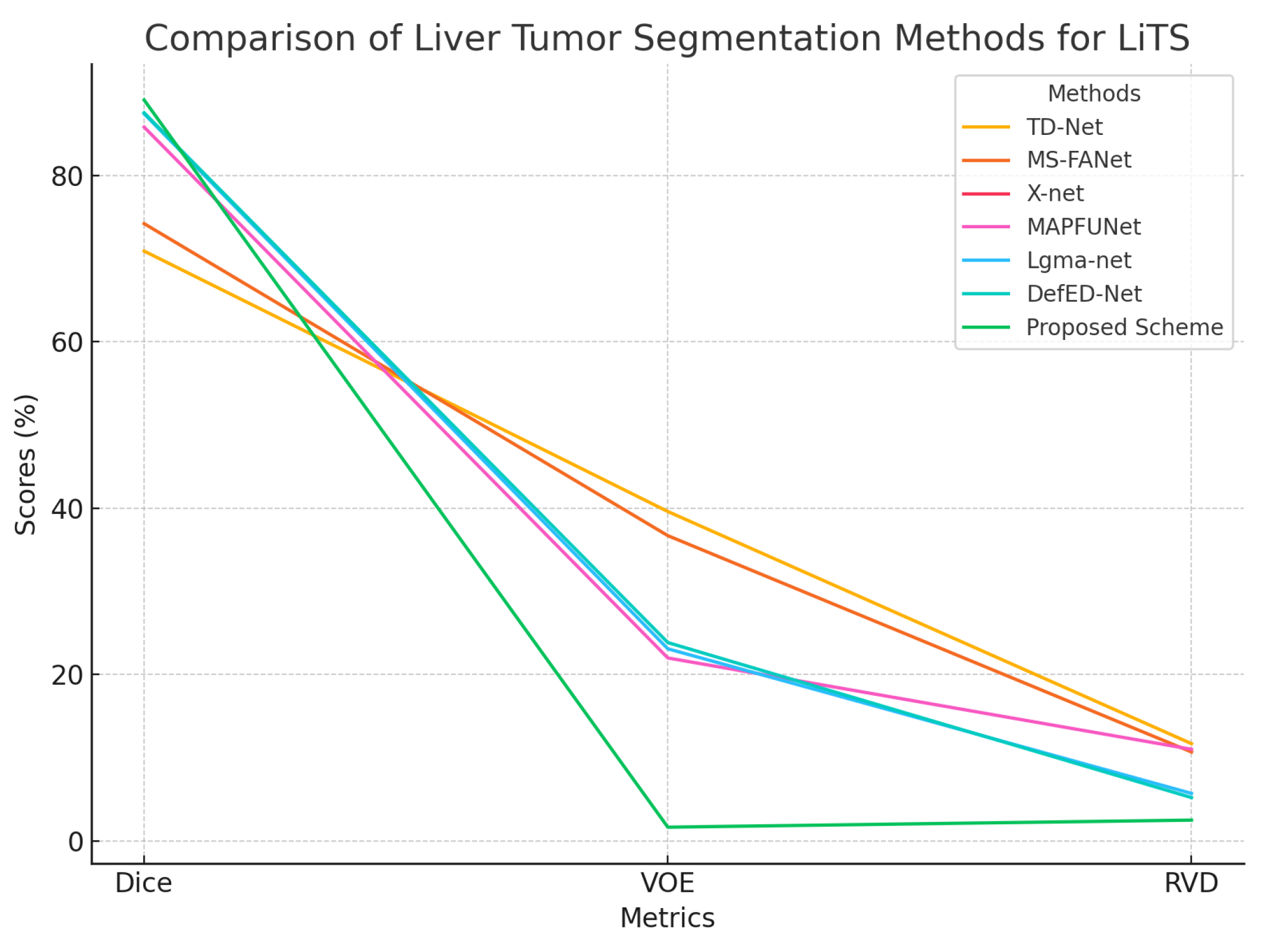
On the LiTS dataset, the proposed scheme achieves a Dice score of 89.06%, which is substantially higher than other state-of-the-art methods, including DefED-Net (87.52%) and MAPFUNet (85.8%). This represents a significant improvement in segmentation accuracy. The VOE is drastically reduced to 1.66%, outperforming the next best value of 22.0% achieved by MAPFUNet, and is much lower than values observed in other methods like TD-Net (39.6%) and MS-FANet (36.7%). Similarly, the RVD of 2.51% represents a considerable improvement over previous methods such as DefED-Net (5.22%) and Lgma-net (5.72%). These results demonstrate that the proposed Swin-UNet achieves highly accurate segmentation with minimal overlap and volume estimation errors.
Figure 8.
Graphical representation of segmentation results on the LiTS dataset.
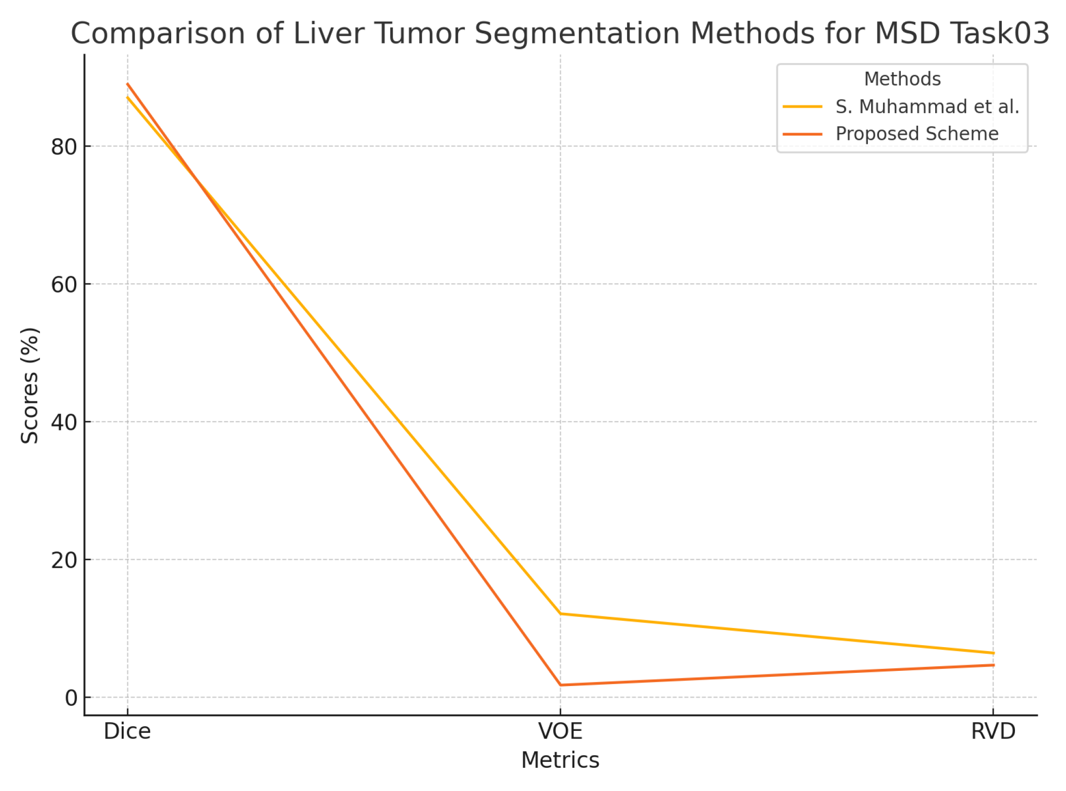
For the MSD Task03 dataset, the proposed Swin-UNet achieves an impressive Dice score of 88.95%, surpassing the existing method by S. Muhammad et al. (87.0%). The VOE is reduced to 1.73%, compared to 12.09% for Muhammad et al., demonstrating a substantial improvement in segmentation precision. The RVD of 4.63% also shows a noticeable improvement over the previous result of 6.39%, further reinforcing the accuracy of the proposed model.
Figure 9.
Graphical representation of segmentation results on the MSD Task03 dataset.
The proposed Swin-UNet model establishes new state-of-the-art results on the LiTS and MSD Task03 datasets, excelling in all performance metrics. For the 3DIRCADb dataset, it delivers the lowest VOE while maintaining competitive Dice and RVD values. These results highlight the proposed model’s ability to segment liver tumors with high accuracy, minimal overlap errors, and precise volume estimation, establishing it as a highly effective solution for medical imaging tasks.
6. Conclusions
This work presented an optimized Swin-UNet model for liver tumor segmentation, specifically designed for deployment on memory-constrained edge devices. By introducing a quadratic penalty objective function and employing the SAR algorithm for hyperparameter optimization, the model effectively balanced segmentation accuracy and model size, making it suitable for real-time applications on devices with limited computational power. The integration of AUC focal loss addressed class imbalance, enhancing the segmentation of minority class pixels in medical images. Experimental results on multiple datasets demonstrated that the optimized model outperformed its larger, unoptimized counterparts in terms of model size, while maintaining competitive performance or even surpassing the unoptimized model in some metrics. This approach facilitated accurate, real-time liver tumor segmentation while ensuring data security and energy efficiency, positioning it as a valuable solution for clinical applications in under-resourced or remote healthcare environments.
Author Contributions
Wail M. Idress contributed to the majority of the work, taking responsibility for conceptualization, methodology, software, validation, formal analysis, investigation, data curation, original draft preparation, review and editing, visualization, and project administration. Yu-Qian Zhao provided supervision, contributed to project administration, and critically reviewed the manuscript. Sayyed Shahid Hussain contributed to the formal analysis and validation. Laeeq Aslam contributed to conceptualization, methodology, software development, formal analysis and funding acquisition. Muhammad Asim provided resources, contributed to data curation, and secured funding. Sajid Shah contributed to investigation and funding acquisition. Mohammed ELAffendi assisted with validation, review and editing, and funding acquisition. All authors have read and agreed to the published version of the manuscript. Please refer to the CRediT taxonomy for detailed role explanations.
Funding
The authors would like to thank Prince Sultan University for paying the APC of this article.Moreover this work was also supported by the Joint Funds of the National Natural Science Foundation of China (Grant No. U23B2063) and the National Natural Science Foundation of China (Grant No. 62076256)
Data Availability Statement
Data used in this study are public datasets and are available.
Acknowledgments
This work was supported by EIAS Data Science Lab, College of Computer and Information Sciences, Prince Sultan University. The authors would like to thanks Prince Sultan University for their support.
Conflicts of Interest
“The authors declare no conflicts of interest.
References
- Sung, H.; Ferlay, J.; Siegel, R.; Laversanne, M.; Soerjomataram, I.; Jemal, A.; et al. Global cancer statistics 2020: GLOBOCAN estimates of incidence and mortality worldwide for 36 cancers in 185 countries. CA: A Cancer Journal for Clinicians 2021, 71, 209–249. [Google Scholar] [CrossRef]
- Kazi, I.A.; Jahagirdar, V.; Kabir, B.W.; Syed, A.K.; Kabir, A.W.; Perisetti, A. Role of Imaging in Screening for Hepatocellular Carcinoma. Cancers 2024, 16, 3400. [Google Scholar] [CrossRef] [PubMed]
- Dharaneswar, S.; Kumar, B.S. Elucidating the novel framework of liver tumour segmentation and classification using improved Optimization-assisted EfficientNet B7 learning model. Biomedical Signal Processing and Control 2025, 100, 107045. [Google Scholar] [CrossRef]
- Ghobadi, V.; Ismail, L.I.; Hasan, W.Z.W.; Ahmad, H.; Ramli, H.R.; Norsahperi, N.M.H.; Tharek, A.; Hanapiah, F.A. Challenges and solutions of deep learning-based automated liver segmentation: A systematic review. Computers in Biology and Medicine 2025, 185, 109459. [Google Scholar] [CrossRef] [PubMed]
- Rahman, H.; Aoun, N.B.; Bukht, T.F.N.; Ahmad, S.; Tadeusiewicz, R.; Pławiak, P.; Hammad, M. Automatic Liver Tumor Segmentation of CT and MRI Volumes Using Ensemble ResUNet-InceptionV4 Model. Information Sciences 2025, 121966. [Google Scholar] [CrossRef]
- Hammad, M.; ElAffendi, M.; Asim, M.; Abd El-Latif, A.A.; Hashiesh, R. Automated lung cancer detection using novel genetic TPOT feature optimization with deep learning techniques. Results in Engineering 2024, 24, 103448. [Google Scholar] [CrossRef]
- Rehman, A.; Mujahid, M.; Damasevicius, R.; Alamri, F.S.; Saba, T. Densely convolutional BU-NET framework for breast multi-organ cancer nuclei segmentation through histopathological slides and classification using optimized features. CMES-Computer modeling In engineering and sciences. 2024, 141, 2375–2397. [Google Scholar] [CrossRef]
- Hussain, S.S.; Degang, X.; Shah, P.M.; Islam, S.U.; Alam, M.; Khan, I.A.; Awwad, F.A.; Ismail, E.A. Classification of Parkinson’s disease in patch-based MRI of substantia nigra. Diagnostics 2023, 13, 2827. [Google Scholar] [CrossRef]
- Javed, R.; Saba, T.; Alahmadi, T.J.; Al-Otaibi, S.; AlGhofaily, B.; Rehman, A. EfficientNetB1 Deep Learning Model for Microscopic Lung Cancer Lesion Detection and Classification Using Histopathological Images. Computers, Materials & Continua 2024, 81. [Google Scholar]
- Gul, S.; Khan, M.S.; Bibi, A.; Khandakar, A.; Ayari, M.A.; Chowdhury, M.E. Deep learning techniques for liver and liver tumour segmentation: A review. Computers in Biology and Medicine 2022, 147, 105620. [Google Scholar] [CrossRef]
- Moghe, A.A.; Singhai, J.; Shrivastava, S. Automatic threshold based liver lesion segmentation in abdominal 2D-CT images. International Journal of Image Processing (IJIP) 2011, 5, 166. [Google Scholar]
- Peng, W.; Zhao, Y. Liver CT image segmentation based on modified Canny algorithm. In Proceedings of the 2019 12th International Congress on Image and Signal Processing, BioMedical Engineering and Informatics (CISP-BMEI). IEEE; 2019; pp. 1–5. [Google Scholar]
- Anter, A.; Hassenian, A. CT liver tumor segmentation hybrid approach using neutrosophic sets, fast fuzzy c-means and adaptive watershed algorithm. Artif. Intell. Med. 2019, 97, 105–117. [Google Scholar] [CrossRef]
- Xu, Y.; Quan, R.; Xu, W.; Huang, Y.; Chen, X.; Liu, F. Advances in medical image segmentation: A comprehensive review of traditional, deep learning and hybrid approaches. Bioengineering 2024, 11, 1034. [Google Scholar] [CrossRef] [PubMed]
- Al-Kofahi, Y.; Lassoued, W.; Lee, W.; Roysam, B. Improved automatic detection and segmentation of cell nuclei in histopathology images. IEEE Trans Biomed Eng 2010, 57, 841–852. [Google Scholar] [CrossRef]
- Kong, H.; Akakin, H.; Sarma, S. A generalized Laplacian of Gaussian filter for blob detection and its applications. IEEE Trans Cybern 2013, 43, 1719–1733. [Google Scholar] [CrossRef]
- Basu, M. Gaussian-based edge-detection methods-a survey. IEEE Trans Syst Man Cybern Part C (appl Rev) 2002, 32, 252–260. [Google Scholar] [CrossRef]
- Chan, T.; Vese, L. Active contours without edges. IEEE Trans Image Process 2001, 10, 266–277. [Google Scholar] [CrossRef]
- Moga, A.; Gabbouj, M. Parallel marker-based image segmentation with watershed transformation. J Parallel Distrib Comput 1998, 51, 27–45. [Google Scholar] [CrossRef]
- Saha Roy, S.; Roy, S.; Mukherjee, P.; Roy, A. An automated liver tumour segmentation and classification model by deep learning based approaches. Comput. Methods Biomech. Biomed. Eng. Imaging Vis. 2022, 1–13. [Google Scholar] [CrossRef]
- Chen, Y.; et al. MS-FANet: multi-scale feature attention network for liver tumor segmentation. Computers in Biology and Medicine 2023, 163, 107208. [Google Scholar] [CrossRef]
- Lakshmi, P.; Sampurna, P.; et al. Deploying the model of improved heuristic-assisted adaptive SegUnet++ and multi-scale deep learning network for liver tumor segmentation and classification. J. Real-Time Image Process. 2025, 22, 8. [Google Scholar] [CrossRef]
- Reyad, M.; et al. Architecture optimization for hybrid deep residual networks in liver tumor segmentation using a GA. Int. J. Comput. Intell. Syst. 2024, 17, 209. [Google Scholar] [CrossRef]
- Di, S.; et al. TD-Net: A hybrid end-to-end network for automatic liver tumor segmentation from CT images. IEEE Journal of Biomedical and Health Informatics 2022, 27, 1163–1172. [Google Scholar] [CrossRef]
- Liu, Z.; et al. PA-Net: A phase attention network fusing venous and arterial phase features of CT images for liver tumor segmentation. Comput. Methods Programs Biomed. 2024, 244, 107997. [Google Scholar] [CrossRef] [PubMed]
- Valanarasu, J.; Oza, P.; Hacihaliloglu, I.; Patel, V. Medical transformer: Gated axial-attention for medical image segmentation. In Proceedings of the Proc. Med. Image Comput. Comput. Assist. Interv. 2021; pp. 36–46. [Google Scholar]
- Dosovitskiy, A.; et al. An image is worth 16×16 words: Transformers for image recognition at scale. In Proceedings of the Proc. 9th Int. Conf. Learn. Representations; 2021; pp. 1–22. [Google Scholar]
- Zhu, X.; Su, W.; Lu, L.; Li, B.; Wang, X.; Dai, J. Deformable DETR: Deformable transformers for end-to-end object detection. In Proceedings of the Proc. Int. Conf. Learn. Representations; 2021; pp. 1–16. [Google Scholar]
- Liang, J.; Homayounfar, N.; Ma, W.C.; Xiong, Y.; Hu, R.; Urtasun, R. PolyTransform: Deep polygon transformer for instance segmentation. In Proceedings of the Proc. IEEE/CVF Conf. Comput. Vis. Pattern Recognit. 2020; pp. 9128–9137. [Google Scholar]
- Balasubramanian, P.; Lai, W.C.; Seng, G.; Selvaraj, J. APESTNet with Mask R-CNN for liver tumour segmentation and classification. Cancers 2023, 15, 330. [Google Scholar] [CrossRef] [PubMed]
- Chen, J.; et al. TransUNet: Transformers make strong encoders for medical image segmentation. arXiv:2102.04306, arXiv:2102.04306 2021.
- Ni, Y.; et al. DA-Tran: Multiphase liver tumor segmentation with a domain-adaptive transformer network. Pattern Recognition 2024, 149, 110233. [Google Scholar] [CrossRef]
- Vaswani, A.; Shazeer, N.; Parmar, N.; Uszkoreit, J.; Jones, L.; Gomez, A.N.; Kaiser, L.; Polosukhin, I. Attention is all you need. Advances in Neural Information Processing Systems 2017, 30. [Google Scholar]
- Alexey, D. An image is worth 16x16 words: Transformers for image recognition at scale. arXiv preprint arXiv: 2010.11929, arXiv:2010.11929 2020.
- Liu, Z.; Lin, Y.; Cao, Y.; Hu, H.; Wei, Y.; Zhang, Z.; Xie, Z.; Lin, S.; Li, H. Swin Transformer: Hierarchical Vision Transformer using Shifted Windows. Proceedings of the IEEE/CVF International Conference on Computer Vision (ICCV), 2021; 10012–10022. [Google Scholar]
- Ronneberger, O.; Fischer, P.; Brox, T. U-Net: Convolutional Networks for Biomedical Image Segmentation. International Conference on Medical Image Computing and Computer-Assisted Intervention (MICCAI), 2015; 234–241. [Google Scholar]
- Shabani, A.; Asgarian, B.; Salido, M.; Gharebaghi, S.A. Search and rescue optimization algorithm: A new optimization method for solving constrained engineering optimization problems. Expert Systems with Applications 2020, 161, 113698. [Google Scholar] [CrossRef]
- Bilic, P.; Christ, P.; Li, H.B.; Vorontsov, E.; Ben-Cohen, A.; Kaissis, G.; Menze, B.H. The liver tumor segmentation benchmark (LiTS). Medical Image Analysis 2023, 84, 10268. [Google Scholar] [CrossRef]
- Soler, L.; Hostettler, A.; Agnus, V.; Charnoz, A.; Fasquel, J.B.; Moreau, J.; Marescaux, J. 3D image reconstruction for comparison of algorithm database, 2010.
- Antonelli, M.; Reinke, A.; Bakas, S.; Farahani, K.; Kopp-Schneider, A.; Landman, B.A.; Cardoso, M.J. The medical segmentation decathlon. Nature Communications 2022, 13, 4128. [Google Scholar] [CrossRef]
- Lei, T.; et al. DefED-Net: Deformable encoder-decoder network for liver and liver tumor segmentation. IEEE Transactions on Radiation and Plasma Medical Sciences 2021, 6, 68–78. [Google Scholar] [CrossRef]
- Chi, J.; et al. X-Net: Multi-branch UNet-like network for liver and tumor segmentation from 3D abdominal CT scans. Neurocomputing 2021, 459, 81–96. [Google Scholar] [CrossRef]
- Ren, W.; et al. Lgma-net: liver and tumor segmentation methods based on local–global feature mergence and attention mechanisms. Signal, Image and Video Processing 2025, 19, 1–11. [Google Scholar] [CrossRef]
- Kushnure, D.T.; Talbar, S.N. MS-UNet: A multi-scale UNet with feature recalibration approach for automatic liver and tumor segmentation in CT images. Computerized Medical Imaging and Graphics 2021, 89, 101885. [Google Scholar] [CrossRef]
- Sun, J.; et al. MAPFUNet: Multi-attention Perception-Fusion U-Net for Liver Tumor Segmentation. Journal of Bionic Engineering, 2024; 1–25. [Google Scholar]
- Muhammad, S.; Zhang, J. Segmentation of Liver Tumors by Monai and PyTorch in CT Images with Deep Learning Techniques. Applied Sciences 2024, 14, 5144. [Google Scholar] [CrossRef]
Figure 1.
Block diagram of the proposed methodology for optimizing Swin-UNet for liver cancer segmentation.
Figure 1.
Block diagram of the proposed methodology for optimizing Swin-UNet for liver cancer segmentation.
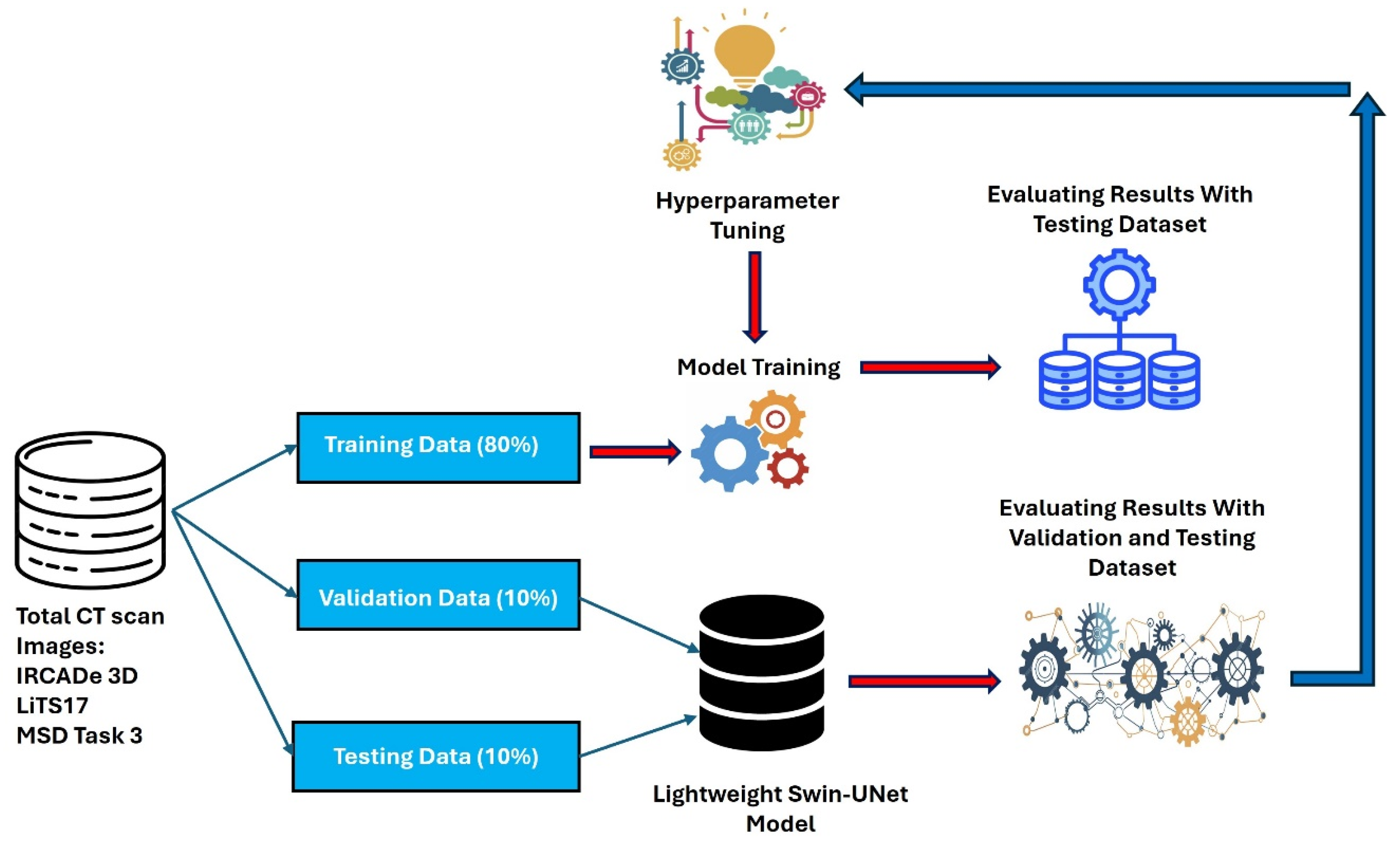
Figure 2.
Swin Unet Architecture.
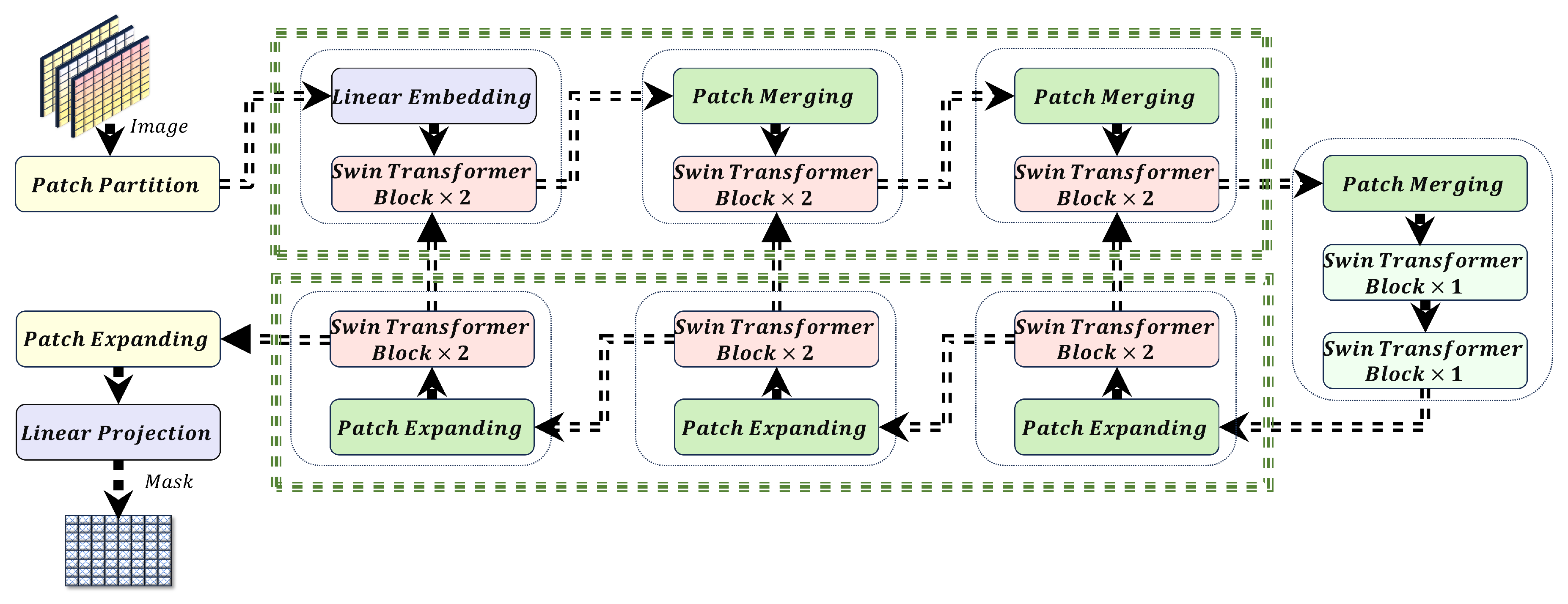
Figure 3.
Block diagram of the proposed hyper-parameter optimization using the SAR algorithm and training with AUC focal loss.
Figure 3.
Block diagram of the proposed hyper-parameter optimization using the SAR algorithm and training with AUC focal loss.
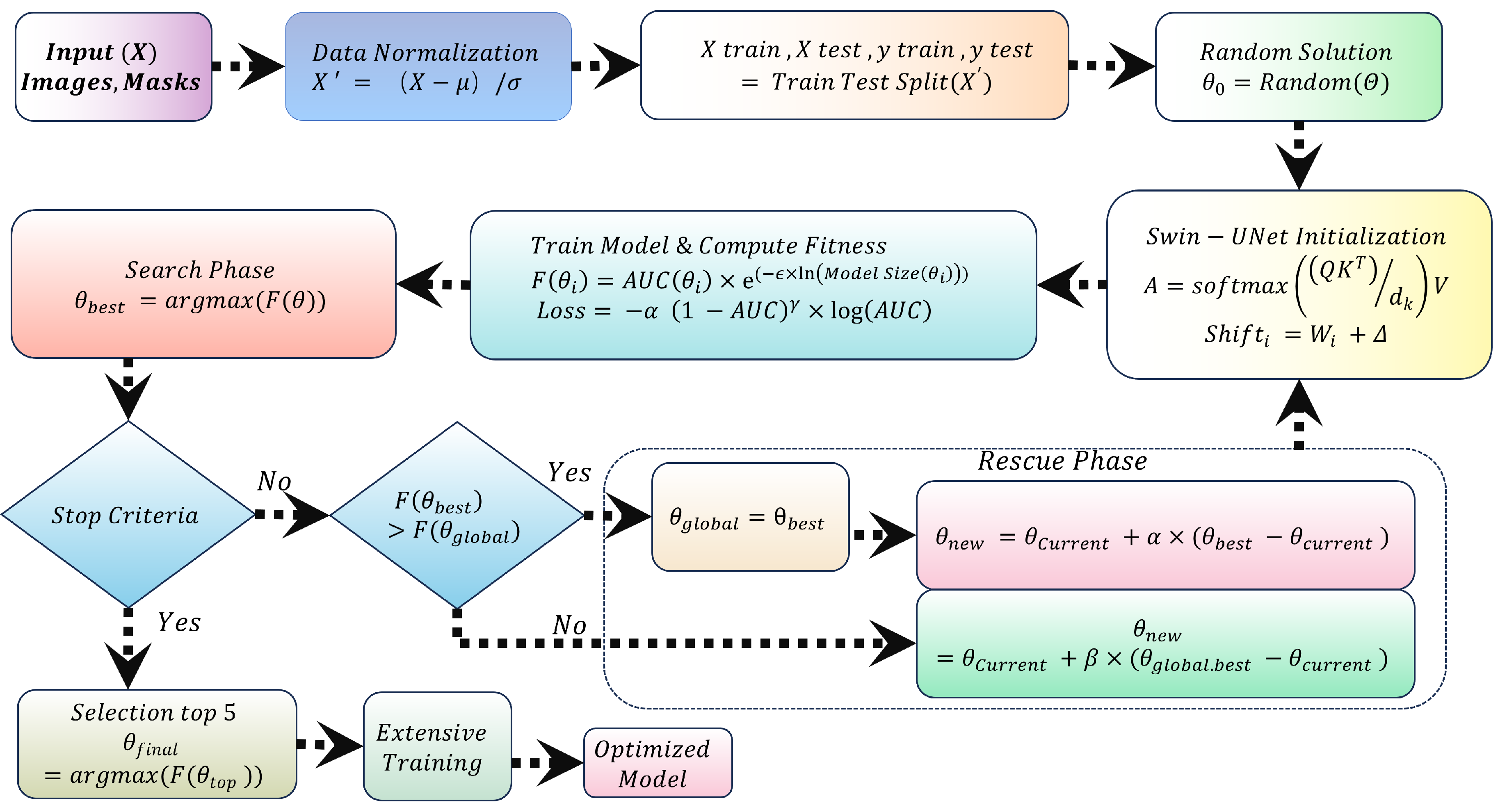
Figure 4.
Visual Results of Segmentation with Different Values on IRCADe 3D Dataset.
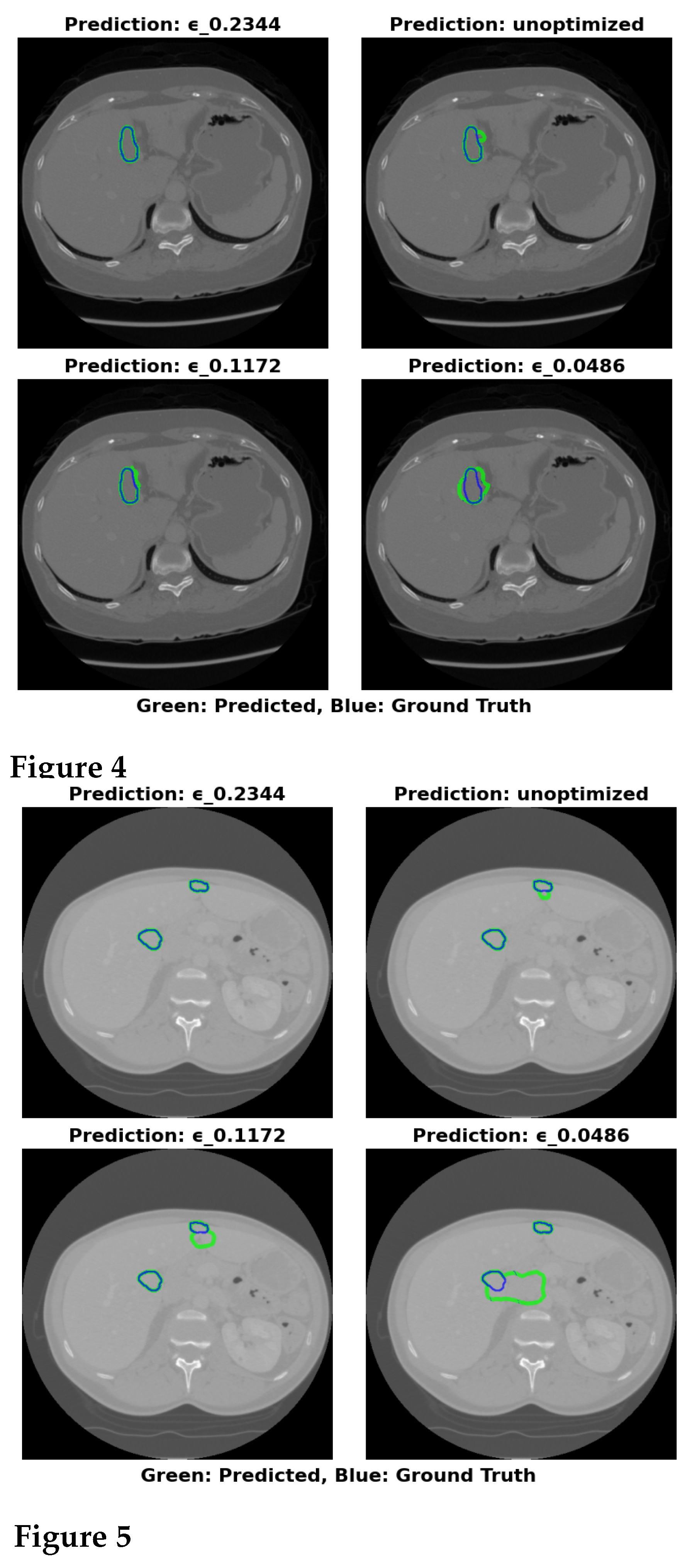
Figure 5.
Visual Results of Segmentation with Different Values on LiTS17 Dataset.
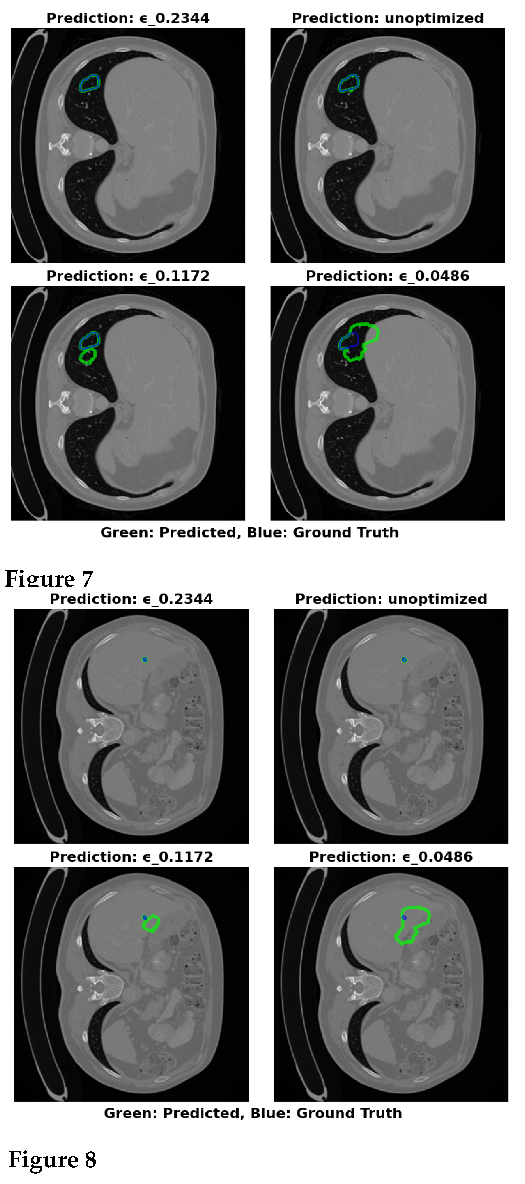
Figure 6.
Visual Results of Segmentation with Different Values on MSD Dataset.
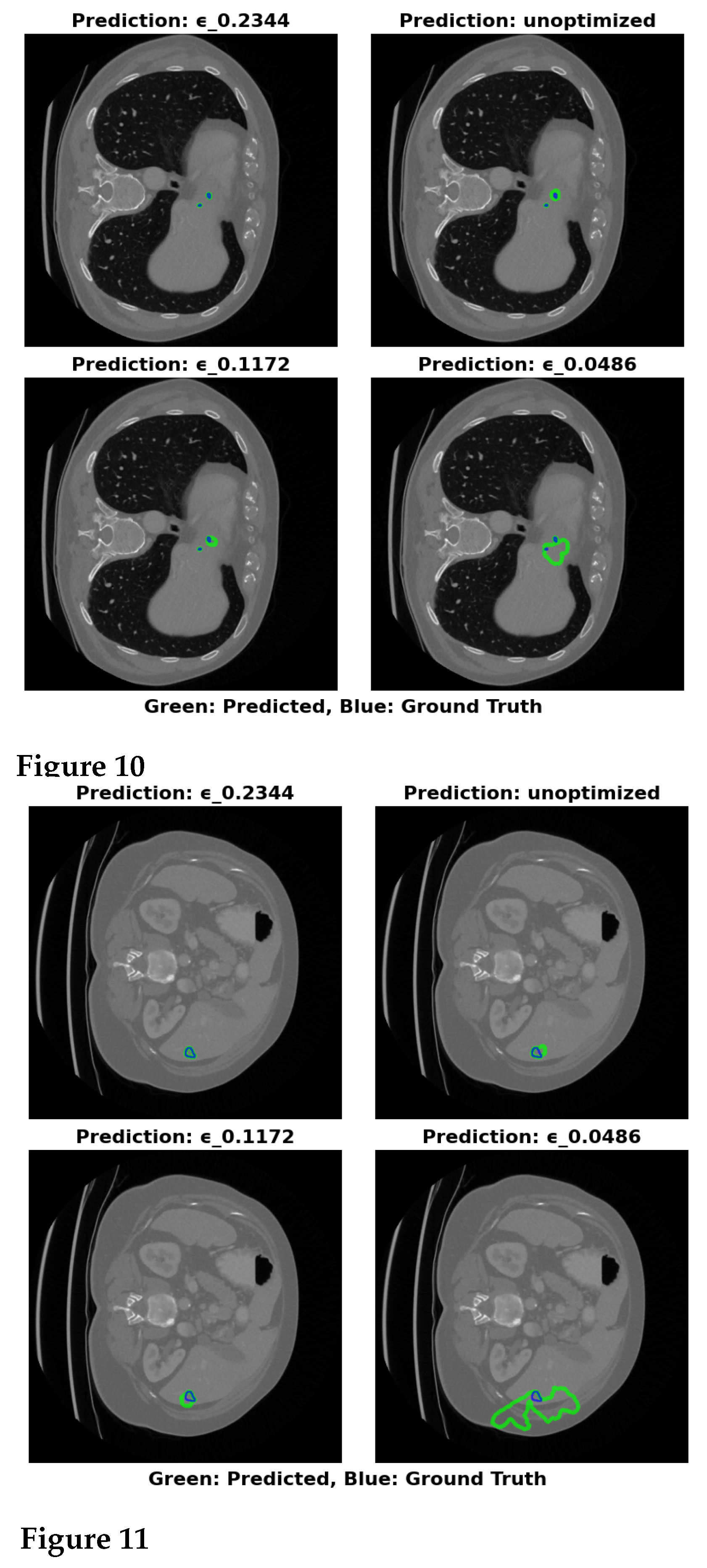
Figure 7.
Graphical representation of segmentation results on the 3DIRCADb dataset.
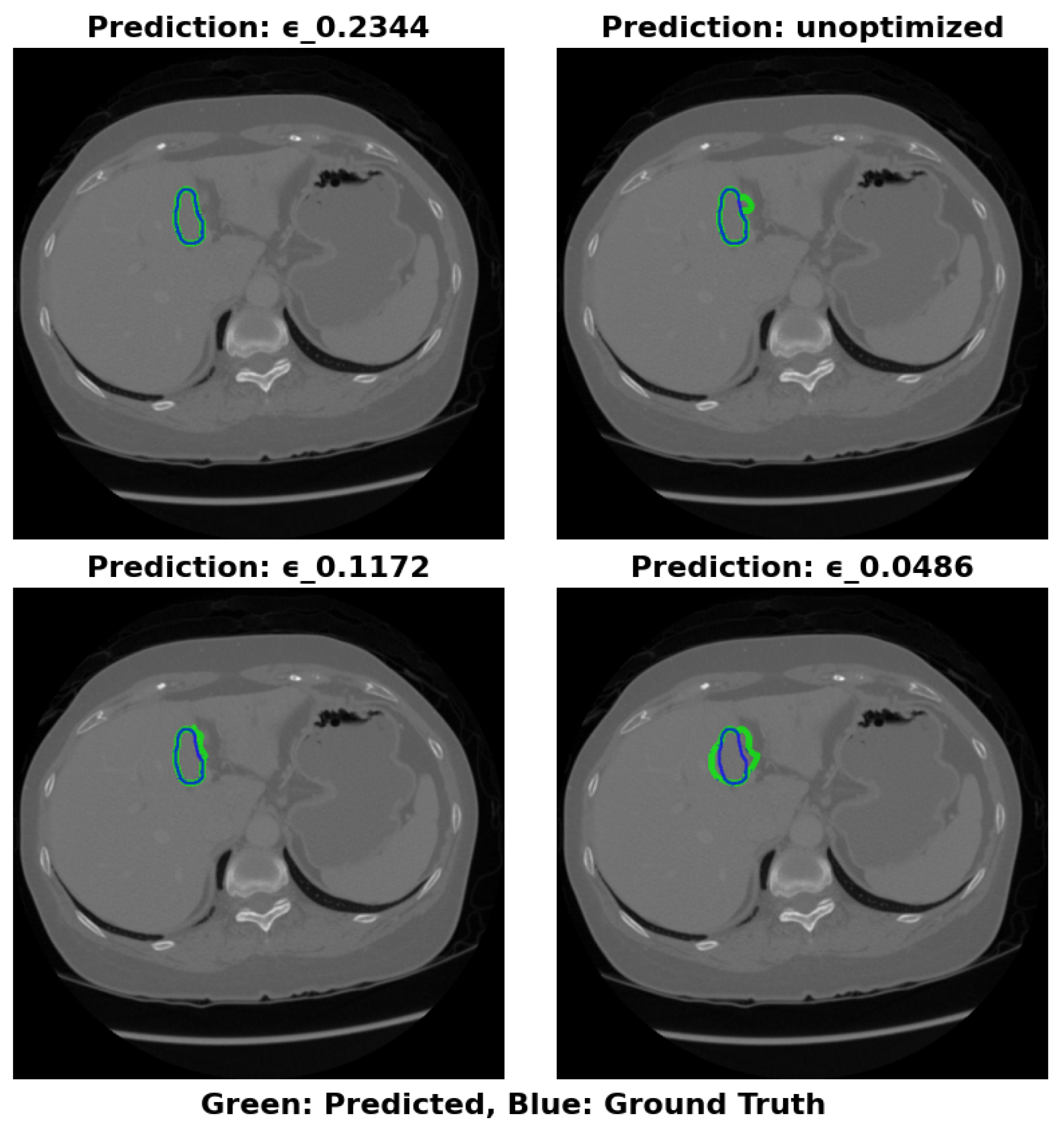
Table 1.
Hyperparameter constraints for the Swin-UNet model and AUC focal loss.
| Hyperparameter | Symbol | Range |
|---|---|---|
| Depth | D | [2, 8] |
| Initial Filter Number | [32, 256] | |
| Patch Size | P | [2, 16] |
| Number of Attention Heads | H | [1, 16] |
| Window Size | W | [1, 8] |
| MLP Size | M | [32, 512] |
| AUC Focal Loss Alpha | [0, 5] | |
| AUC Focal Loss Gamma | [0, 5] |
Table 2.
Dataset Distribution for Liver Tumor Segmentation.
| Dataset | Total Images | Training (80%) | Validation (10%) | Test (10%) |
|---|---|---|---|---|
| LiTS17 [38] | 131 | 104 | 13 | 13 |
| IRCADe 3D [39] | 20 | 16 | 4 | 4 |
| MSD Task-3 [40] | 131 | 104 | 13 | 13 |
| Total | 282 | 224 | 30 | 30 |
Table 3.
Summary of Model Hyperparameters and Setup.
| Hyperparameter | Value |
|---|---|
| Learning Rate | 0.0001 |
| Epochs | 2000 |
| Batch Size | 64 |
| Optimizer | Adam |
| Patience (Early Stopping) | 10 epochs |
| Device for Optimization | Nvidia 3090 Ti |
| Device for Deployment | Jetson Nano |
Table 5.
Performance Metrics Across Configurations and Datasets.
| Dataset | Size (MB) | Acc. | Prec. | Rec. | Spec. | Dice | VOE | RVD(%) | |
|---|---|---|---|---|---|---|---|---|---|
| 3DIRCADb | unoptimized | 324.91 | 0.9985 | 0.8272 | 0.8488 | 0.9999 | 0.8340 | 0.1801 | 0.30 |
| 3DIRCADb | 0.2344 | 64.16 | 0.9998 | 0.9297 | 0.9915 | 1.0000 | 0.9478 | 0.0783 | 0.23 |
| 3DIRCADb | 0.1172 | 30.88 | 0.9976 | 0.7423 | 0.8401 | 0.9994 | 0.7891 | 0.2661 | 0.89 |
| 3DIRCADb | 0.0486 | 17.22 | 0.9962 | 0.7400 | 0.8329 | 0.9962 | 0.7644 | 0.2634 | 4.82 |
| LiTS | unoptimized | 324.91 | 0.9998 | 0.9797 | 0.9709 | 1.0000 | 0.8753 | 0.0291 | 2.89 |
| LiTS | 0.2344 | 64.16 | 0.9999 | 0.9923 | 0.9910 | 1.0000 | 0.8906 | 0.0166 | 2.51 |
| LiTS | 0.1172 | 30.88 | 0.9996 | 0.9288 | 0.9817 | 0.9998 | 0.8405 | 0.0791 | 3.17 |
| LiTS | 0.0486 | 17.22 | 0.9987 | 0.8724 | 0.9925 | 0.9988 | 0.7998 | 0.1345 | 16.8 |
| MSD Task03 | unoptimized | 324.91 | 0.9999 | 0.9712 | 0.9921 | 0.9999 | 0.8758 | 0.0366 | 19.33 |
| MSD Task03 | 0.2344 | 64.16 | 0.9999 | 0.9906 | 0.9920 | 1.0000 | 0.8895 | 0.0173 | 4.63 |
| MSD Task03 | 0.1172 | 30.88 | 0.9999 | 0.9569 | 0.9921 | 0.9999 | 0.8654 | 0.0508 | 27.39 |
| MSD Task03 | 0.0486 | 17.22 | 0.9964 | 0.8124 | 0.9933 | 0.9965 | 0.8363 | 0.1938 | 48.04 |
Table 6.
Comparison of Liver Tumor Segmentation Methods across Datasets in terms of Dice, VOE and RVD.
Table 6.
Comparison of Liver Tumor Segmentation Methods across Datasets in terms of Dice, VOE and RVD.
| Dataset | Method/Scheme | Dice (%) | VOE (%) | RVD (%) |
|---|---|---|---|---|
| 3DIRCADb | DefED-Net [41] | 66.2 | 34.3 | 0.8 |
| X-net [42] | 69.1 | 36.1 | 0.7 | |
| TD-Net [24] | 68.2 | 40.8 | 8.4 | |
| MS-FANet [21] | 78.0 | 31.3 | 15.5 | |
| Lgma-net [43] | 83.2 | 24.3 | 0.76 | |
| MS-UNet [44] | 84.1 | 27.3 | 0.22 | |
| MAPFUNet [45] | 85.9 | 23.7 | 0.22 | |
| Proposed Scheme | 94.78 | 7.83 | 0.23 | |
| LiTS | TD-Net [24] | 70.9 | 39.6 | 11.7 |
| MS-FANet [21] | 74.2 | 36.7 | 10.7 | |
| X-net [42] | 76.4 | - | - | |
| MAPFUNet [45] | 85.8 | 22.0 | 11.02 | |
| Lgma-net [43] | 87.4 | 23.1 | 5.72 | |
| DefED-Net [41] | 87.52 | 23.85 | 5.22 | |
| Proposed Scheme | 89.06 | 1.66 | 2.51 | |
| MSD Task03 | S. Muhammad et al. [46] | 87.0 | 12.09 | 6.39 |
| Proposed Scheme | 88.95 | 1.73 | 4.63 |
Disclaimer/Publisher’s Note: The statements, opinions and data contained in all publications are solely those of the individual author(s) and contributor(s) and not of MDPI and/or the editor(s). MDPI and/or the editor(s) disclaim responsibility for any injury to people or property resulting from any ideas, methods, instructions or products referred to in the content. |
© 2025 by the authors. Licensee MDPI, Basel, Switzerland. This article is an open access article distributed under the terms and conditions of the Creative Commons Attribution (CC BY) license (http://creativecommons.org/licenses/by/4.0/).
Copyright: This open access article is published under a Creative Commons CC BY 4.0 license, which permit the free download, distribution, and reuse, provided that the author and preprint are cited in any reuse.


