
Submitted:
11 March 2025
Posted:
11 March 2025
You are already at the latest version
Abstract
Leaf Area Index (LAI) is one of the key parameters for characterizing leaf density, vegetation growth status, and canopy structure. Rapid, objective, and accurate acquisition of forest LAI is of great significance for studying forest ecosystems and forestry production. This study focuses on the core issue of accurately segmenting leaf elements from background elements in hemispherical photography used for forest LAI measurement, with a particular focus on meeting the real-time requirements of embedded platforms. The differences in grayscale values and frequency characteristics between leaf regions, trunk regions, and sky regions in vegetation canopy images were leveraged to decompose, process, and reconstruct such images using a 9/7 wavelet-based transformation method, achieving efficient and precise segmentation of leaf regions. Through the extraction of canopy gap fraction, rapid LAI measurement was enabled. Comparative experimental results showed that the proposed inversion method exhibited a high correlation with the LAI-2200C measurement results (r=0.847, RMSE=0.431), fully verifying its accuracy across different forest ecological environments. This study provides strong support for the development of portable, high-precision LAI measurement devices and holds practical application value and broad application prospects.
Keywords:
Leaf Area Index
; Hemispherical Photography
; Image Segmentation
; Wavelet Transform
1. Introduction
Forests are an essential part of global vegetation, widely distributed across various climatic and soil conditions. They play an irreplaceable role in maintaining ecological balance, preserving biodiversity, regulating climate, and providing resources for humanity [1,2,3]. As a key component of Earth’s life-support system and sustainable human development, forests are increasingly challenged by rapid population growth, urbanization, and modernization. Balancing forest ecological protection with technological advancements has become a pressing issue. Strengthening forestry research, advancing forestry science and technology, and enhancing forest monitoring and assessment are crucial research topics in forestry and environmental protection. Efficient vegetation information statistics are a key aspect of this process. They are vital for understanding forest vegetation growth, accurately assessing forest ecological quality, scientifically formulating conservation strategies, and optimizing forestry production layouts [4]. Vegetation indices serve as an essential tool for measuring vegetation conditions, directly reflecting growth status, coverage, and ecological functions. They provide a simple and effective empirical measure of surface vegetation conditions and are widely applied in land cover analysis, vegetation classification, and environmental change monitoring. By analyzing vegetation time-series data, researchers can assess ecosystem health and stability, indirectly reflecting biodiversity changes. This is significant for natural resource management and ecological balance maintenance [5,6]. Additionally, as a crucial tool in ecological research, vegetation indices support scientific studies by offering data and insights, promoting further ecological research development.
The concept and development of vegetation indices date back to the late 1960s to the early 1990s. In 1969, Jordan proposed the first vegetation index—Ratio Vegetation Index (RVI)—which calculates the reflectance ratio between the near-infrared and red bands [7]. In 1972, Pearson et al. introduced the Vegetation Index Number (VIN), furthering vegetation index research [8]. In 1973, Rouse et al. applied a nonlinear normalization process to RVI, resulting in the Normalized Difference Vegetation Index (NDVI) [9], which later became widely used in vegetation remote sensing [10]. To date, over 40 vegetation indices have been defined globally, covering parameters such as vegetation coverage, chlorophyll content, and canopy structure [11,12].
The Leaf Area Index (LAI) is one of the fundamental parameters describing canopy structure. It is defined as half the total leaf surface area per unit ground area [13]. LAI reflects leaf quantity, distribution, and canopy density and is crucial for studying plant growth, photosynthesis, transpiration, and crop yield [14,15]. It has broad applications and research value in forestry and agriculture [16]. Accurate measurement and analysis of LAI enable a better understanding of plant health and growth, providing a scientific basis for forestry and agricultural management [17,18,19,20].
The measurement methods for LAI primarily include direct and indirect approaches [21]. The direct measurement method involves collecting plant leaf samples, measuring their area, and calculating the total leaf area per unit of land to determine LAI. Although this method is accurate, it is labor-intensive, and the collection of leaf samples can cause some damage to the plants. It is typically suitable for small-scale or specific-area measurements and is difficult to apply over large areas [22]. In contrast, the indirect measurement method estimates LAI by measuring parameters such as canopy reflectance and transmittance using remote sensing technology and optical instruments, combined with mathematical models [23,24]. This approach offers advantages such as fast measurement speed, wide coverage, and the ability to conduct large-scale measurements quickly without damaging trees, saving both labor and resources. As a result, it is widely used for LAI measurement [25].
Measurement methods based on radiative transfer models estimate LAI indirectly by simulating light transmission characteristics within plant canopies. Common instruments include TRAC, AccuPAR, and the LAI-2000 series plant canopy analyzers [26,27,28]. These instruments provide high measurement accuracy and are suitable for various types of vegetation, geographical regions, and ecosystems. However, radiative transfer models often rely on certain assumptions (e.g., uniform canopy structure, single leaf morphology), which may reduce their applicability in complex environments, thereby affecting the ac-curacy of LAI estimation. Additionally, radiative transfer models are highly sensitive to environmental factors such as light conditions, weather, and atmospheric conditions. They require high-precision optical sensors to capture the optical properties of plant canopies, which often come with high costs and technical requirements, increasing the barrier to their use [29].
In recent years, the hemispherical photography-based LAI measurement method has gained significant attention among researchers, driven by advancements in image processing technology [29]. This approach involves capturing canopy images from beneath the vegetation using a fisheye lens-equipped camera. By applying image segmentation techniques, the method distinguishes leaf areas (target pixels) from gaps (sky pixels) and estimates LAI using radiative transfer models or empirical models. Compared to traditional radiative transfer model-based methods, hemispherical photography offers the advantage of permanently documenting vegetation dynamics, providing valuable visual data for long-term research and enabling the tracking of canopy changes over time [30,31,32]. Additionally, it is more cost-effective and easier to operate than high-precision optical sensors, making it a practical choice for large-scale ecological monitoring.
The integration of artificial intelligence and automated image analysis software has further enhanced the efficiency of this method [33], enabling rapid processing of large datasets and extraction of canopy structural information for LAI estimation. However, challenges remain in practical applications. Image segmentation accuracy can be compromised by variable lighting conditions and image quality, particularly in dense forests or complex ecosystems, where distinguishing between leaf and sky pixels becomes difficult [34,35,36]. These limitations highlight the need for continued refinement of the technique to improve robustness and reliability in diverse environmental conditions.
The accuracy of vegetation image segmentation algorithms significantly impacts the precision of hemispherical photography-based LAI measurements. Currently, commonly used image segmentation algorithms primarily include color-based segmentation algorithms and deep learning-based segmentation algorithms. Color-based segmentation algorithms typically rely on grayscale features of images, with common methods including threshold segmentation and edge detection [37,38]. These algorithms are relatively simple in structure and computationally efficient, but they are sensitive to factors such as image noise and lighting variations, resulting in limited adaptability to complex scenes and segmentation accuracy [39,40]. Additionally, these algorithms struggle to effectively distinguish between leaf areas and trunk areas, often leading to overestimation of the leaf area index. In contrast, deep learning-based segmentation algorithms utilize convolutional neural networks for feature extraction and classification, enabling them to handle complex image segmentation tasks with higher accuracy and processing efficiency. However, these algorithms require substantial computational resources during both training and inference, necessitating high-performance computing hardware. Moreover, the performance of these models heavily depends on the quality and quantity of annotated datasets. Yet, there is currently no publicly available standardized annotated dataset, which limits the further application and development of these algorithms to some extent. As a result, deep learning-based methods remain largely in the experimental research phase and are not yet practical for rapid field measurements [41,42].
This study introduces a wavelet-based segmentation paradigm addressing these methodological gaps [43,44,45]. Through multi-scale 9/7 wavelet decomposition, the algorithm simultaneously analyzes grayscale textures and frequency-domain features of canopy components, effectively handling complex forest textures while suppressing noise artifacts. A novel dynamic optimization suppression method improves segmentation precision by adaptively adjusting coefficient thresholds, overcoming the rigidity of conventional fixed-threshold approaches. Experimental validation against LAI-2200C benchmark measurements demonstrates enhanced accuracy across diverse ecosystems, with comparative analysis revealing significant improvements over traditional color-based segmentation in handling mixed-pixel scenarios and structural interference.
The proposed methodology advances LAI quantification by synergizing multi-resolution image analysis with adaptive threshold optimization, particularly effective in heterogeneous canopies where conventional methods struggle [46]. While maintaining computational practicality for field applications, this approach ad-dresses critical limitations in current segmentation techniques through its inherent noise resilience and multi-scale feature discrimination capabilities. The integration of wavelet transforms with dynamic suppression mechanisms establishes a new framework for vegetation analysis, bridging the gap between computationally intensive deep learning methods and oversimplified traditional algorithms.
2. Materials and Methods
2.1. Study Area and Data Source
2.1.1. Study Area
The study selects three forest ecosystems from different geographic regions within China as study areas: Jiangshanjiao Experimental Forest Farm, Forestry Academy of Heilongjiang Province (43°85’N, 128°95’E), Qianyanzhou Subtropical Forest Ecosystem Observation Station, Chinese Academy of Sciences (26°75’N, 115°06’E), and the Qingshui River campus of the University of Electronic Science and Technology of China in Chengdu, Sichuan Province (30°75’N, 103°93’E). The study area map is shown in Figure 1. The Jiangshanjiao observation station mainly includes temperate mixed forests of larch, red pine, white birch, and mountain ash, while the Qianyanzhou station mainly consists of subtropical evergreen broadleaf forests of oil tea, citrus, and fir trees. The observation site at the University of Electronic Science and Technology includes subtropical evergreen broadleaf forests with camphor, nanmu, and Osmanthus trees.
Each study area has significant differences in climate, soil types, etc., with diverse vegetation types, densities, and heights, aiming to comprehensively evaluate the stability, adaptability, and accuracy of the inversion method proposed in this study when dealing with different vegetation types under varying ecological conditions. An overview of the study areas is shown in Table 1.
2.1.2. Data Collection
This experiment employs a self-developed vegetation image acquisition system, synchronized with the LAI-2200C instrument, to capture high-resolution canopy images, as illustrated in Figure 2. The vegetation image acquisition device is an embedded device that integrates image capture and storage functions. It is equipped with an STM32F767 microprocessor, a CMOS image sensor OV2640, and a 160° ultra-wide-angle fisheye lens (in comparison, the LAI-2200C has a field of view of 148°), capable of capturing images with up to 2 million pixels. The device is designed to be compact and lightweight, supporting both independent and synchronized collection with the LAI-2200C. During synchronized collection, the device is secured to the optical probe of the LAI-2200C using Velcro straps to ensure the alignment of the fisheye lens center with the center of the optical sensor of the LAI-2200C.
When measuring, the vegetation image acquisition device and LAI-2200C are connected via a cable, and each time the LAI-2200C takes a measurement, the vegetation image device synchronously captures a hemispherical canopy image, which is stored on the built-in TF card of the device. This method ensures that measurements are taken at the same time and location for the same target, effectively reducing the influence of environmental factors on the results and enhancing data accuracy and reliability.
Measurements were conducted in flat areas within the experimental zone using a 6*3 grid sampling method. Specifically, six sample points were collected along the diagonal direction of each sampling area at equal intervals, with a minimum spacing of 10 meters between sampling points. As shown in Figure 3, the green background represents the sampling area, and the red dots indicate the sample collection points. To minimize single-measurement errors and ensure the stability and accuracy of the data, each sample point was measured three times. Due to the unique characteristics of forest vegetation, trees within the measured area grow non-uniformly, potentially creating irregular gaps of varying sizes, which appear as irregular blank regions in the canopy images.
2.1.3. Dataset
This study collected 60 sets of data, with 20 sets from each study area. Each data set includes one LAI-2200C measurement file and 21 vegetation canopy hemispherical images (3 images are of the outside vegetation, and 18 are of the vegetation canopy). The sample data is shown in Figure 4. The LAI-2200C measurement file contains information such as firmware version, file creation time, GPS log, and LAI calculation results [47]. It is important to note that during the measurement process, the LAI-2200C computes the overall LAI of the area by averaging the results of each sample point within a specific sampling region, and generates a measurement file based on this data. In this study, the arithmetic mean of the LAI calculated from the 18 vegetation canopy images was used to represent the measurement results of the inversion method proposed in this paper. This approach ensured a comprehensive consideration of all sample data, effectively reflecting the overall variation in the leaf area index across the sampling area and providing an objective benchmark for evaluating the performance of the inversion method.
2.2. Principles of Wavelet Image Decomposition and the 9/7 Wavelet
Wavelet transform is a very useful technique in image processing. Through wavelet transform, images can be decomposed into different scales and frequency components, allowing information extraction in both spatial and frequency domains. This characteristic makes wavelet transform excellent in many image processing tasks, especially in areas such as image compression, denoising, feature extraction, and segmentation. Applying wavelet decomposition to an image allows for the extraction of information at different frequencies, as shown in Figure 5.
A first wavelet transform of the image results in four subbands: low-low (), low-high (), high-low (), and high-high (). These subbands represent the features of the image at different frequencies and directions. The subband contains the main low-frequency information of the image, reflecting the main structure and background, representing the primary features of the image. The , , and subbands contain high-frequency information in the horizontal, vertical, and diagonal directions, representing details and edges in the image. To extract finer features and improve segmentation accuracy, the subband undergoes further wavelet transformation, resulting in four additional subbands that provide a deeper decomposition.
In wavelet image decomposition, selecting an appropriate transformation method and basis function is crucial for effective image processing. The type of wavelet basis and the level of decomposition depend on the application needs and objectives. In LAI measurement, it is important to emphasize the high-frequency features of leaf areas. Therefore, wavelet decomposition is often carried out at deeper levels to better extract detailed information and suppress low-frequency background interference. The 9/7 wavelet transform is a high-precision, energy-concentrated wavelet transform method with relatively low computational complexity and excellent compression performance. It effectively retains image details and has good edge preservation capability, making it highly suitable for complex background and edge-blurring image segmentation tasks.
Additionally, the 9/7 wavelet transform can be efficiently implemented using only basic addition, subtraction, and bit-shift operations, significantly simplifying the computational process and minimizing storage requirements. This computational efficiency makes the 9/7 wavelet transform particularly well-suited for deployment on resource-constrained microprocessor platforms, enabling high-performance, real-time image processing even in low-power environments.
2.3. Imaging Region Extraction
Fisheye lenses typically consist of a group of very short focal length convex lenses. When light passes through them, it refracts at different angles. The refracted light is projected onto the image in a circular field of view, as shown in Figure 6(a). Due to misalignment during installation, the circular field of view is not exactly centered on the photo. The position of the circular region’s center and its radius must be determined. A white background image is captured using the vegetation image acquisition device, and this fisheye image is then binarized, as shown in Figure 6(b). Next, morphological operations are performed to smooth the boundaries and extract the boundary points, yielding the circle’s center (840, 634) and radius , as shown in Figure 6(c).
According to the equidistant projection model of the fisheye lens, a Cartesian coordinate system is established with the center of the circular imaging area as the origin. The zenith angle of any pixel on the image is calculated a using the following formula:
2.4. Analysis of Vegetation Canopy Image Feature
The hemispherical photography method involves capturing canopy images from be-low the plant canopy using a camera equipped with a fisheye lens, with a viewing angle range from 180° to 200°, where the foreground is vegetation and the background is the sky, as shown in Figure 7(a). The canopy image consists of three regions: the leaf area, the trunk area, and the sky area, which exhibit significant differences in grayscale and frequency. The leaf area has a higher reflectance, finer texture, and is primarily concentrated in high-frequency bands after wavelet transformation. The trunk area is typically darker, with the lowest grayscale and weaker reflection, mainly concentrated in low-frequency bands. The sky area is well-lit, with the highest grayscale, generally appearing in the canopy gaps, and corresponds to the image’s low-frequency information. By performing wavelet transformation, the vegetation image is decomposed into low-frequency and high-frequency subbands. The high-frequency components retain the leaf area details, while the low-frequency components capture the main structure of the trunk and sky. Therefore, by utilizing the different characteristics of these three regions, 9/7 wavelet transformation is employed for multi-scale decomposition of the vegetation image, enhancing or suppressing certain frequency components to increase the grayscale difference between the regions. Finally, threshold segmentation is used to reconstruct the image, achieving segmentation of specific vegetation regions.
The wavelet decomposition results of the vegetation image in Figure 7(a) are shown in Figure 7(b) and Figure 7(c). After the first wavelet decomposition, the component retains much of the structural information, with the leaf, trunk, and sky regions still clearly visible. This demonstrates that the first wavelet transformation effectively preserves the image’s low-frequency information and presents the main structure of the image. The and components contain significant boundary information for the leaf and trunk areas, with sparse leaf information. After a second wavelet decomposition, the high-frequency information is increasingly decomposed, and the leaf area information in the component decreases, while trunk and sky information is largely preserved. A substantial amount of leaf information is decomposed into , , and parts, displaying high brightness, while the trunk and sky areas appear in black, with significant grayscale differences between adjacent regions.
The wavelet decomposition results of the vegetation image show that the frequency information differs significantly across the regions. The leaf area typically exhibits strong high-frequency features, while the trunk and sky areas are concentrated in low-frequency components. In the hemispherical photography method for measuring LAI, attention is focused on the proportion of the leaf area in the entire image. Therefore, by suppressing the low-frequency components and enhancing the grayscale value of the leaf area, the leaf region becomes more prominent in the image, achieving segmentation of the leaf area. This method not only improves segmentation efficiency but also adapts well to images under varying lighting conditions, making it highly adaptable. This frequency-based segmentation algorithm provides a new and effective technical route for LAI measurement using hemispherical photography.
2.5. LAI Extraction
The LAI inversion method based on hemispherical photography extracts vegetation parameter information by analyzing canopy images. This process includes two key steps: image segmentation and LAI extraction. Image segmentation refers to distinguishing different regions (leaf area, trunk area, and sky area) within the image. The segmented leaf area provides the data foundation for subsequent LAI calculation. LAI extraction is achieved by estimating the proportion of the leaf area in the image.
2.5.1. Image Segmentation
As analyzed previously, vegetation images exhibit distinct frequency characteristics: leaf areas are typically associated with high-frequency components, while trunk and sky regions are dominated by low-frequency components. Accurate segmentation of leaf areas is critical for precise LAI measurement, as it provides the foundational data required for reliable calculations. To achieve this, wavelet decomposition is applied to the vegetation image, with a focus on suppressing low-frequency components. This suppression minimizes the influence of background elements (e.g., trunks and sky) on leaf area segmentation, thereby enhancing the grayscale contrast between leaf regions and other parts of the image. The improved contrast facilitates the effective application of image segmentation algorithms, enabling more accurate extraction of leaf areas and ultimately contributing to higher precision in LAI estimation.
2.5.1.1 Fixed Coefficient Suppression
The vegetation image is decomposed using two layers of 9/7 wavelet transform. The pixel values within the effective imaging area of the subband from the second wavelet decomposition are normalized:
where is the original grayscale pixel value of the image, ranging from , and is the normalized pixel value, ranging from . A coefficient I is applied to globally suppress the grayscale values of the normalized subband:
The purpose of global grayscale suppression is to enhance the high-frequency components by reducing the low-frequency components, thereby highlighting the edges and details of the leaf area. During this process, the grayscale values of the low-frequency components (trunk and sky areas) are lowered, making the leaf area more distinct in the subsequent image segmentation process. After suppression, the subband is reconstructed with the other subbands using the inverse 9/7 wavelet transform. Finally, Otsu’s method is used to perform automatic threshold segmentation, yielding clear image segmentation results.
Global grayscale suppression was applied to the vegetation image shown in Figure 8(a) using coefficients , and . The segmentation results are displayed in Figure 8, where the trunk and sky regions are marked in white, and the leaf areas are marked in black. It is important to note that smaller suppression coefficients result in stronger suppression effects on the image.
By comparing the segmentation results, the following five observations can be made:
- (1)
- When the vegetation image is directly processed using Otsu’s method, some of the brighter leaf areas are misclassified as the sky, and some darker trunk areas are misclassified as leaf areas due to insufficient grayscale contrast.
- (2)
- After the wavelet transformation of the image, Otsu’s method accurately segments the trunk area.
- (3)
- When the suppression coefficient is too small (), some leaf areas with subtle grayscale variations are misclassified as sky regions, as shown in the red-circled areas in Figure 8(b), Figure 8(c), and Figure 8(d). This occurs because these leaf areas, located in the low-frequency components, experience excessive suppression, reducing their grayscale values to levels similar to other low-frequency areas, resulting in misclassification.
- (4)
- As the suppression coefficient increases, the grayscale suppression of low-frequency components weakens, improving the contrast between the leaf area and the sky area, thereby enhancing the leaf area segmentation.
- (5)
- When the suppression coefficient is excessively large , the sky region is erroneously classified as part of the leaf area, as illustrated in the blue-circled region of Figure 9(d). This misclassification arises because the high grayscale values of the sky are inadequately suppressed, diminishing the grayscale contrast between the sky and the leaf area and resulting in segmentation errors.
When collecting vegetation images in natural environments, factors such as weather conditions, leaf density, and distribution differences result in significant global grayscale variations across different vegetation images. The low-frequency components of the image may include the leaf area, sky area, and trunk area. Due to these variations in grayscale distribution, the same suppression coefficient may produce inconsistent results across different images, leading to under-suppression or over-suppression in some images, affecting the accuracy of segmentation results. Therefore, when applying grayscale suppression, it is beneficial to consider a suppression scheme based on the image’s grayscale mean to improve segmentation accuracy.
2.5.1.2 Grayscale Mean-Based Suppression
For vegetation images, after performing the two-layer 9/7 wavelet decomposition, all pixel values in the effective imaging area of the subband are normalized as . By iterating through all pixel points, the arithmetic mean of the normalized grayscale image is calculated as follows:
where N represents the number of pixel points within the effective imaging area. Global grayscale suppression is applied to the normalized subband using the coefficient I as follows:
The suppressed subband is then reconstructed with the other subbands using the inverse 9/7 wavelet transform. Finally, Otsu’s method is used to segment the reconstructed image automatically.
Subsequently, the suppressed subband, denoted as , along with the other subbands, is reconstructed into an image using the inverse 9/7 wavelet transform. Finally, Otsu’s method is employed to perform automatic threshold segmentation on the reconstructed image, yielding clear and precise image segmentation results.
For the vegetation image shown in Figure 9(a), global grayscale suppression is applied with coefficients , with the segmentation results shown in the Figure 9. The trunk and sky areas are marked in white and the leaf area in black. It should be noted that the smaller the suppression coefficient, the stronger the suppression effect on the image.
Segmentation results show that the grayscale mean-based suppression algorithm still provides good segmentation results. However, some leaf areas with smooth grayscale transitions are still misclassified as sky regions. Compared with the fixed coefficient global suppression algorithm, the following two differences were observed:
- (1)
- When the suppression coefficient does not exceed , the sky region is correctly segmented without misclassification.
- (2)
- When the suppression coefficient increases to , the sky region is misclassified as part of the leaf area.
The analysis of the two suppression algorithms yields the following conclusions:
- (1)
- The trunk area in vegetation images typically has the lowest grayscale values, and even with a high suppression coefficient, it is correctly identified without misclassification.
- (2)
- When the suppression coefficient is too small, the suppression effect on low-frequency components is too strong, causing some gently varying leaf areas to be overly suppressed, making them indistinguishable from the sky, leading to misclassification.
- (3)
- When the suppression coefficient is too large, the sky area is not effectively suppressed, reducing the contrast between the sky and leaf areas and causing misclassification of the sky as the leaf area.
- (4)
- An appropriate suppression coefficient creates a clear grayscale contrast between the leaf area, sky, and trunk, improving segmentation accuracy.
Thus, there is an optimal suppression coefficient. If the coefficient is too low, it can effectively identify the sky area; however, if it is too high, the ability to recognize the sky decreases, though misclassification of the leaf area improves. Based on this analysis, a dynamic optimal suppression coefficient algorithm is proposed. This algorithm adapts to complex vegetation image segmentation needs, ensuring accurate segmentation results under various conditions.
2.5.1.3 Dynamic Optimization of Suppression
Dynamic optimization of suppression is an algorithm that dynamically adjusts the suppression coefficient. Through multiple dynamic iterations, the algorithm gradually approaches the optimal suppression coefficient to adapt to the grayscale characteristics of different vegetation images, enabling more accurate image segmentation. This provides precise data for subsequent LAI extraction. The algorithm process is shown in Figure 10.
The vegetation image undergoes a two-level 9/7 wavelet decomposition, and all pixel values within the effective imaging region of the subband from the second-level decomposition are normalized as .The arithmetic mean of the normalized grayscale images calculated as . Suppression coefficients and are defined such that:
where C is a positive increment. These coefficients are applied to globally suppress the normalized and subband:
The suppressed subbands and are then reconstructed with other subbands using the 9/7 inverse wavelet transform, yielding reconstructed grayscale images and . Finally, Otsu’s method is applied for automatic threshold segmentation to obtain clear segmentation results.
White pixels (sky and trunk regions) are labeled as 1, and black pixels (leaf regions) as 0. The number of white pixels in and , denoted and are counted. The difference between the two images is calculated as:
During execution, the algorithm repeats or terminates based on the value of . If iteration is required, increases by a step size :
when is small, the segmentation results of and are similar (). As increases, may misclassify sky regions as leaf regions earlier than , causing to decrease sharply while remains stable. A sudden increase in indicates optimal suppression coefficients have been reached, terminating the optimization.
To address potential misclassification of leaf regions as sky in (due to small ), is used to correct . A pure sky image (vegetation-free) is normalized:
where is the original grayscale (range: ). represents the normalized pixel value, scaled to the range . By iterating through all pixel points, the arithmetic mean of the normalized grayscale values for the vegetation-free image is calculated as follows:
For each white pixel in , if the corresponding pixel in is black (non-trunk) and the original pixel’s grayscale is less than , the pixel is corrected to black (leaf region).
2.5.1.4 Segmentation Performance Evaluation
To objectively compare the three 9/7 wavelet-based image segmentation algorithms, three evaluation metrics are used: Difference Index between Regions (), Within-Region Variance Consistency (), and Maximum Contrast within Regions (). The definitions of these metrics are detailed below.
quantifies the grayscale or texture differences between distinct regions in an image. A higher value indicates greater inter-region differences and better segmentation performance. The is defined as:
where (leaf, trunk, and sky regions); is the number of region combinations; and are the maximum and minimum grayscale values in the effective image area; is the average grayscale of region i.
evaluates the uniformity of grayscale distribution within a region. A higher value indicates lower intra-region variability and better segmentation. is defined as:
where N is the total number of pixels in the effective area of the vegetation image; denotes the k-th segmented region; is the pixel count of region and represents the grayscale value of pixel i. Due to the inherent elemental heterogeneity of leaf regions, the metric is computed exclusively for assessing consistency within the sky and trunk regions.
The metric quantifies grayscale value differences within a specific region of an image. It focuses on intra-region brightness contrast, evaluating the intensity of texture, detail, or variation. In vegetation image processing, is used to assess contrast differences between regions. A smaller value indicates lower maximum contrast variability in the k-th region, signifying better segmentation for that region. Similarly, a smaller value reflects better overall segmentation performance. is defined as:
where is defined as:
where : Total number of regions (leaf, trunk, sky): is the k-th segmented region; refers to the total pixels in region; is the grayscale value of pixel i and W(i) means the neighborhood of pixel i.
2.5.2. LAI Extraction
2.5.2.1 LAI Extraction Method
The hemispherical photography-based LAI inversion method relies on vegetation parameter retrieval algorithms derived from canopy gap fraction theory, grounded in the Beer-Lambert theorem [48] and probabilistic models of leaf distribution. The core formula is:
where : Zenith angle; : Gap fraction (porosity); : Projection function.
In practical processing, to improve measurement efficiency, n equidistant zenith angles are typically selected. For each angular ring, the average canopy gap fraction is measured, and the results are weighted and summed to compute the final LAI. The discretized formula is:
where : Weighting factor for angle ; : Angular interval between adjacent angles; : Normalized weighting factor, satisfying . This leads to the fast-calculation formula for multi-angle LAI inversion:
In this study, five zenith angles are selected:7°, 23°, 38°, 53°, and 68° (identical to the LAI-2200C instrument). The normalized weighting factors for each angle are provided in Table 2.
2.5.2.2 Evaluation of LAI Extraction Results
To assess the performance of the comparative experiments, three statistical metrics were selected: correlation coefficient (r), and p-value [51]. The r measures the strength and direction of the linear relationship between datasets. A larger absolute r value indicates stronger correlation. The formula for r is:
where: : Predicted value, i.e., the inversion result from the Dynamic Optimization Suppression method. : Mean of the predicted values (average of the inversion results from the Dynamic Optimization Suppression method). : True observed value, i.e., the measurement from the LAI-2200C. : Mean of the true observed values (average of the LAI-2200C measurements). n: Total number of observation points ( n = 60 in this study).
The p-value is used to test whether there are statistically significant differences between variables. If , no statistically significant difference exists between the datasets. If : A statistically significant difference is observed. The p-value is typically derived from statistical hypothesis testing. Different statistical tests correspond to distinct p-value calculation formulas. In this study, T-test is employed to compute the p-value.
3. Results
3.1. Dynamic Optimal Suppression Algorithm Segmentation Results and Evaluation
3.1.1. Dynamic Optimal Suppression Algorithm Reconstruction Results
Set the suppression coefficient , with an increment of 0.001, and use the dynamic optimal suppression method to decompose, reconstruct, and repair the vegetation image shown in Figure 11(a). The final output result is shown in Figure 11(d). In Figure 11(a), the leaf area within the red circle was misclassified as the sky area in Figure 11(b). Using Figure 11(c) to repair Figure 11(b), the result in Figure 11(d) correctly identifies the leaf area within the red circle. Meanwhile, the reconstruction results of other similar areas in Figure 11(d) also show varying degrees of improvement. Therefore, the dynamic optimal suppression method can handle complex vegetation images, reduce misclassification, and optimize the overall segmentation effect through the repair step.
3.1.2. Dynamic Optimal Suppression Algorithm Segmentation Results
To evaluate the segmentation results of the image color-based segmentation algorithm and the three wavelet transform-based segmentation algorithms mentioned earlier, Otsu’s method, the fixed coefficient suppression algorithm (), the grayscale mean-based suppression algorithm (), and the dynamic optimal suppression algorithm were applied to segment the vegetation image shown in Figure 12(a). The results are shown in Figure 12. Otsu’s method suffers from misclassification in images with complex backgrounds or regions with unclear contrast differences. The fixed coefficient suppression algorithm and grayscale mean-based suppression algorithm experience over-suppression, resulting in less accurate segmentation. The dynamic optimal suppression algorithm significantly improves the misclassification situations, providing better segmentation results compared to the fixed coefficient suppression algorithm and the grayscale mean-based suppression algorithm, thus further improving the segmentation accuracy.
3.1.3. Dynamic Optimal Suppression Algorithm Segmentation Result Evaluation
3.1.3.1 Evaluation of LAI Extraction Results
The segmentation result evaluation indicators for the fixed coefficient suppression algorithm (), grayscale mean-based suppression algorithm (), and dynamic optimal suppression algorithm for the vegetation image shown in Figure 10(a) are listed in Table 3. The dynamic optimal suppression algorithm has the largest region difference index DIR, indicating that the difference between the three regions in its reconstruction result is the greatest. It also has the largest variance consistency index Ui, meaning that the internal variation of the reconstructed regions is the smallest. Both the maximum contrast index within a single region and the overall maximum contrast index are the smallest, indicating that the contrast variation within the regions is the smallest. Moreover, as the suppression coefficient increases, the segmentation effect of the same algorithm improves, but the segmentation effect for the trunk area remains similar. In conclusion, the dynamic optimal suppression algorithm achieves the best segmentation results for this vegetation image.
3.1.4. Multi-Sample Evaluation Statistics
To further verify that the dynamic optimal suppression algorithm provides the best segmentation results, ten vegetation images were randomly selected, and the segmentation result evaluation indicators for the fixed coefficient suppression algorithm (), grayscale mean-based suppression algorithm (), and dynamic optimal suppression algorithm were calculated, as shown in Table 4. As the sample size increases, some evaluation indicators with larger suppression coefficients show no improvement or even worse segmentation effects (highlighted in blue in Table 4). This is due to the randomness of the samples, which leads to differences in feature distribution and affects the algorithm’s performance. For example, when using the fixed coefficient suppression method with , the overall maximum contrast index increases compared to , indicating that the contrast difference within the segmentation area increases and the segmentation effect worsens. The statistical results show that the dynamic optimal suppression algorithm still outperforms the fixed coefficient suppression algorithm and grayscale mean-based suppression algorithm for the segmentation of these 10 vegetation images, further verifying its advantages in vegetation image segmentation tasks.
3.2. Results and Evaluation of Leaf Area Index Extraction
The dynamic optimal suppression algorithm’s inversion results( abbreviated as LAI-9/7WT) were plotted with the LAI-2200C measurement results on the x-axis and y-axis, respectively, and linear fitting was performed to calculate the r and p- values, as shown in Figure 13. The correlation coefficients for the three test sites were 0.939 (Chengdu), 0.967 (Jiangshanjiao), and 0.931 (Qianyanzhou), with an overall correlation coefficient of 0.847, and p-values all far less than 0.001. The experimental results indicate a highly significant correlation between the inversion method designed in this paper and the LAI-2200C measurement results.
The boxplot of LAI value distribution in the testing area (Figure 14) and the statistical data table of the boxplot (Table 5) are as follows. The median, 75th percentile, and 25th percentile of the three regions are close to LAI-2200C, indicating that the measurement of the dynamic optimization suppression algorithm has a similar distribution. This is consistent with the conclusion reflected in the correlation analysis.
Using the value of LAI-2200C as the true value, calculate the variance performance index of the inversion value of the dynamic optimization suppression algorithm, as shown in Table 6.
4. Discussion
4.1. Discussion on Wavelet Transform-Based Segmentation Algorithms
The fixed coefficient suppression algorithm, when processing images, produces consistent suppression effects on all images due to the fixed suppression coefficient, leading to over-segmentation or misclassification in some images.
The grayscale mean-based suppression algorithm dynamically adjusts based on grayscale mean, improving the image segmentation effect. However, its flexibility is limited, and it has limitations when dealing with complex backgrounds or detailed regions.
The dynamic optimal suppression algorithm dynamically adjusts the suppression coefficient based on image characteristics and performs well for different types of vegetation images. Additionally, using the reconstruction results to repair misclassification can more accurately separate the leaf area, avoid over-suppression issues, and significantly improve the segmentation accuracy and stability. Future work could continue to explore how to further optimize the algorithm to ensure its adaptability and reliability in large-scale or different environments.
4.2. Suppression Coefficient Selection
This paper compares the segmentation results of different suppression coefficients and selects the suppression coefficient parameters based on experience, especially the initial values and , and increment for the dynamic optimal suppression algorithm, which is not universally applicable. In setting the suppression coefficients and , , meaning that the increment of compared to is the same as the increment for itself:
This parameter design borrows from the iterative computing idea, simplifying the computational load. In actual execution, the segmentation result of suppression coefficient is used as the segmentation result for in the next iteration, thus only recalculating the new suppression coefficient ’s result, which reduces computational load by half compared to when .
The advantage of the dynamic optimal suppression algorithm is its ability to adjust the suppression coefficient based on image characteristics, but this process relies on understanding and prior knowledge of image properties. To enhance the algorithm’s adaptability, future research could use automated parameter optimization, machine learning, and multi-scale analysis methods to automatically determine the suppression coefficient parameters, further improving the algorithm’s applicability and reliability.
4.3. Instrument Selection for Comparison
Currently, commonly used indirect measurement instruments are divided into two categories: one category measures the light radiation above or below the vegetation using specific optical sensors, and then estimates the leaf area index based on the light attenuation, with representative instruments including the LAI-2200 series, TRAC, and DEMON; the other category uses optical cameras to obtain hemispherical canopy images and then analyzes the images to calculate the LAI, with representative instruments including the CI-100. Among these instruments, the LAI-2200 series, developed by the U.S. company LI-COR, occupies a crucial position in plant physiology and ecological research due to its efficiency, non-destructive nature, and wide application [29].
The LAI-2200C uses a fisheye optical sensor (vertical field of view of 148°) to measure projected light at 5 zenith angles (7°, 23°, 38°, 53°, 68°) on the canopy, using a vegetation canopy radiation propagation model to calculate the leaf area index. As a high-precision leaf area index measuring instrument, the LAI-2200C has been widely used worldwide and is the instrument of choice for researchers in plant physiology and ecology. Its measurement results are widely recognized within the industry for their high reliability and accuracy and are regarded as the industry standard.
4.4. Result Analysis and Discussion
The experimental results show that the leaf area index extracted by the inversion method designed in this paper is overall smaller than the LAI-2200C measurement results, which is similar to other studies. This discrepancy occurs because the LAI-2200C assumes that tree leaves are optical black bodies, absorbing all light and neglecting reflection and refraction effects between leaves. In reality, tree leaves have certain reflective and transmissive properties, which affect the light propagation within the canopy and consequently the gap rate measurement. This leads to a smaller gap rate and an overestimation of the LAI in the LAI-2200C measurements. Moreover, the LAI-2200C is sensitive to all shading objects in the field of view, including leaves, stems, and branches [52], which are all included in the measurements, causing an overestimation of the LAI.
In this paper’s designed inversion method, the trunk area is treated as a non-leaf area. During actual measurements, the trunk may block some leaf areas, resulting in an under-estimation of the leaf area, and thus the extracted leaf area index is smaller. Therefore, in practical applications, the LAI-2200C measurement results can be combined with the image-based inversion method through weighted averaging or data fusion techniques to obtain more accurate LAI values or verified using destructive sampling or other independent methods (e.g., ground LiDAR) [52,53,54].
4.5. Image Segmentation Method Comparison and Discussion
The hemispherical photography method captures hemispherical canopy images to calculate the leaf area index. Gap rate extraction is one of the key steps in measuring LAI, and its accuracy directly affects the LAI measurement results. Currently, commonly used image processing algorithms include the traditional Otsu’s method and the improved Otsu’s method [56]. Different algorithms exhibit differences and limitations in segmenting leaf and sky pixels, leading to inaccurate gap rate extraction. Four typical forest vegetation canopy images were selected, and the segmentation results using fixed threshold methods (), traditional Otsu’s method, and improved Otsu’s method are shown in Figure 15. The results show that all segmentation algorithms fail to effectively segment the trunk area, and significant differences are present in the segmentation results. Among these methods, the improved Otsu’s method performs the best.
By applying the dynamic optimal suppression algorithm to decompose, reconstruct, and repair these four typical forest vegetation canopy images, and then segmenting them using the fixed threshold method (), traditional Otsu’s method, and improved Otsu’s method[56], the results are shown in Figure 16. The wavelet transform significantly improves the contrast of the target areas, allowing the segmentation algorithms to more accurately separate the leaf area from the background area. Moreover, after wavelet transformation, the segmentation results are more consistent and show significantly better accuracy than those directly processed with these algorithms on the original images. Therefore, combining wavelet transformation with image segmentation algorithms can significantly reduce the complexity of segmentation and improve both efficiency and accuracy.
4.6. Improvement Measures Discussion
The image processing algorithm proposed in this paper is currently implemented on a PC. If this algorithm is to be migrated to a microprocessor platform (such as embedded systems or Raspberry Pi), the primary task is to evaluate the algorithm’s operating speed and resource usage, including processing time, memory usage, and other key indicators. To improve the running efficiency on microprocessors, optimization of both the code (e.g., reducing unnecessary computations, using more efficient algorithms) and hardware (e.g., utilizing specific hardware acceleration features, optimizing memory access patterns) will be necessary.
The image processing algorithm proposed in this paper performs well with the data from the three selected forest experimental areas. However, due to the limited dataset, it is not possible to determine if the algorithm will still show good segmentation results when processing more diverse tree species datasets. Therefore, it is necessary to collect image datasets containing multiple tree species and evaluate the segmentation results, studying the algorithm’s adaptability to different tree species.
Lastly, by comparing the differences between the leaf area index extracted from different tree species and the actual values, the applicability of the inversion method pro-posed in this paper can be evaluated. Furthermore, analyzing possible influencing factors, such as tree structure features, leaf morphology, and distribution, will help better under-stand how these factors affect the leaf area index inversion results. Once these influencing factors are fully understood, the inversion method can be further optimized and improved to enhance its accuracy and robustness.
5. Conclusions
To address the demand for fast and accurate measurement of LAI in forest ecosystems, this paper proposes a LAI inversion method based on 9/7 wavelet transform. This method focuses on the core issue of accurate segmentation of leaf elements and background elements in vegetation canopy images. By utilizing differences in grayscale and frequency features between the leaf area, trunk area, and sky area, the 9/7 wavelet transform is used to decompose, process, and reconstruct vegetation images, achieving efficient and precise segmentation of the leaf area. By extracting the canopy gap rate, rapid LAI measurement is achieved. Since the wavelet transform enhances the grayscale difference between the leaf area and the background areas (trunk area, sky area), the image segmentation algorithms can more easily identify and separate the leaf area, significantly simplifying the segmentation process. Compared to directly using image segmentation algorithms on raw vegetation images, the wavelet transform-based image segmentation algorithm proposed in this paper shows significant advantages, especially in complex backgrounds and different lighting conditions, achieving higher segmentation accuracy.
To validate the effectiveness of the proposed inversion method, three forest experimental areas from different geographic regions were selected, and vegetation canopy images were synchronized with the LAI-2200C. The LAI values for 60 sampling areas were calculated using the proposed method and compared with the LAI-2200C measurements. The results show that the proposed method is highly correlated with the LAI-2200C measurements (, ), indicating that it has high accuracy under different environmental conditions and is a reliable LAI measurement method.
This paper uses an enhanced algorithm to implement wavelet transforms, significantly simplifying the 9/7 wavelet transform’s computation process, making it suitable for real-time applications. The dynamic optimal suppression algorithm’s parameter setup reduces intermediate data during the calculation process, lowering memory and storage requirements, and providing the potential for application on microprocessor platforms. Combining wavelet transforms makes segmentation results consistent across different segmentation algorithms, showcasing the algorithm’s adaptability to complex scenarios. Therefore, the research results not only apply to efficient and high-precision image processing tasks on PC but also provide strong support for developing portable and high-precision LAI measurement devices. As the technology continues to mature and expand, it is expected to have a profound impact on sustainable agriculture, ecological protection, and addressing climate change.
Author Contributions
Conceptualization, P.W. and L.T.; methodology, P.W. and L.T.; software, P.W.; formal analysis, P.W., G.X., and B.G.; writing—original draft preparation, P.W. and X.G.; writing—review and editing, P.W. and X.G.; funding acquisition, L.T. All authors have read and agreed to the published version of the manuscript.
Funding
This work is supported by the Common Application Support Plat form for Land Observation Satellite of National Civil Space Infrastructure of China (Y930280A2F).
Data Availability Statement
Restrictions apply to the availability of these data. Data were obtained from the Information Research Institute, Chinese Academy of Sciences. Data are available with the permission of the Information Research Institute, Chinese Academy of Sciences.
Acknowledgments
We would like to acknowledge the support of the Information Research Institute, Chinese Academy of Sciences. We would like to acknowledge the students in our team.
Conflicts of Interest
The authors declare no conflicts of interest.
References
- Pan, Y.; Birdsey, R.A.; Fang, J.; Houghton, R.; Kauppi, P.E.; Kurz, W.A.; Phillips, O.L.; Shvidenko, A.; Lewis, S.L.; Canadell, J.G. A Large and Persistent Carbon Sink in the World’s Forests. Science 2011, 333, 988–993. [Google Scholar] [CrossRef]
- Davies, S.J.; Abiem, I.; Abu Salim, K.; Aguilar, S.; Allen, D.; Alonso, A.; Anderson-Teixeira, K.; Andrade, A.; Arellano, G.; Ashton, P.S. Forestgeo: Understanding Forest Diversity and Dynamics through a Global Observatory Network. Biol. Conserv. 2021, 253, 108907. [Google Scholar] [CrossRef]
- Liang, J.; Crowther, T.W.; Picard, N.; Wiser, S.; Zhou, M.; Alberti, G.; Schulze, E.D.; McGuire, A.D.; Bozzato, F.; Pretzsch, H. Positive Biodiversity-Productivity Relationship Predominant in Global Forests. Science 2016, 354, aaf8957. [Google Scholar] [CrossRef]
- Huang, Y.; Chen, Y.; Castro-Izaguirre, N.; Baruffol, M.; Brezzi, M.; Lang, A.; Li, Y.; Härdtle, W.; von Oheimb, G.; Yang, X. Impacts of Species Richness on Productivity in a Large-Scale Subtropical Forest Experiment. Science 2018, 362, 80–83. [Google Scholar] [CrossRef] [PubMed]
- Feng, Y.; Schmid, B.; Loreau, M.; Forrester, D.I.; Fei, S.; Zhu, J.; Tang, Z.; Zhu, J.; Hong, P.; Ji, C. Multispecies Forest Plantations Outyield Monocultures across a Broad Range of Conditions. Science 2022, 376, 865–868. [Google Scholar] [CrossRef]
- Mao, Z.; van der Plas, F.; Corrales, A.; Anderson-Teixeira, K.J.; Bourg, N.A.; Chu, C.; Hao, Z.; Jin, G.; Lian, J.; Lin, F. Scale-Dependent Diversity–Biomass Relationships Can Be Driven by Tree Mycorrhizal Association and Soil Fertility. Ecol. Monogr. 2023, 93, e1568. [Google Scholar] [CrossRef]
- Jordan, C.F. Derivation of Leaf Area Index from Quality of Light on the Forest Floor. Ecology 1969, 50, 663–666. [Google Scholar] [CrossRef]
- Person, R. Remote mapping of standing crop biomass for estimation of the productivity of the short-grass Prairie. In Proceedings of the Pawnee National Grasslands, Colorado, 1972.
- Rouse, J.W.; Haas, R.H.; Schell, J.A.; Deering, D.W. Monitoring Vegetation Systems in the Great Plains with ERTS. Earth Resources Technology Satellite 1973, SP-351, 309-317. [Google Scholar]
- Tucker, Compton J. Red and photographic infrared linear combinations for monitoring vegetation. Remote Sensing of Environment 1979, 8, 127–150. [CrossRef]
- Bannari, A.; Morin, D.; Bonn, F.; Huete, A. R. A review of vegetation indices. Remote Sensing Reviews 1995, 13(1–2), 95–120. [Google Scholar] [CrossRef]
- Xue, J.; Su, B. Significant remote sensing vegetation indices: a review of developments and applications. Journal of Sensors 2017, 1–17. [Google Scholar] [CrossRef]
- Chen, J.M.; Black, T.A. Defining Leaf-Area Index for Non-Flat Leaves. Plant Cell Environ 1992, 15, 421–429. [Google Scholar] [CrossRef]
- Perez, G.; Coma, J.; Chafer, M.; Cabeza, L.F. Seasonal influence of leaf area index (LAI) on the energy performance of a green facade. Build. Environ. 2022, 207, 18. [Google Scholar] [CrossRef]
- Cutini, A.; Matteucci, G.; Mugnozza, G.S. Estimation of leaf area index with the LiCor LAI 2000 in deciduous forests. For. Ecol. Manag. 1998, 105, 55–65. [Google Scholar] [CrossRef]
- Clark, D.B.; Olivas, P.C.; Oberbauer, S.F.; Clark, D.A.; Ryan, M.G. First direct landscape-scale measurement of tropical rain forest Leaf Area Index, a key driver of global primary productivity. Ecol. Lett. 2008, 11, 163–172. [Google Scholar] [CrossRef] [PubMed]
- Tian, Y.; Zheng, Y.; Zheng, C.M.; Xiao, H.L.; Fan, W.J.; Zou, S.B.; Wu, B.; Yao, Y.Y.; Zhang, A.J.; Liu, J. Exploring scale-dependent ecohydrological responses in a large endorheic river basin through integrated surface water-groundwater modeling. Water Resour. Res. 2015, 51, 4065–4085. [Google Scholar] [CrossRef]
- Iio, A.; Hikosaka, K.; Anten, N.P.R.; Nakagawa, Y.; Ito, A. Global dependence of field-observed leaf area index in woody species on climate: A systematic review. Glob. Ecol. Biogeogr. 2014, 23, 274–285. [Google Scholar] [CrossRef]
- Taugourdeau, S.; le Maire, G.; Avelino, J.; Jones, J.R.; Ramirez, L.G.; Quesada, M.J.; Charbonnier, F.; Gomez-Delgado, F.; Harmand, J.M.; Rapidel, B. Leaf area index as an indicator of ecosystem services and management practices: An application for coffee agroforestry. Agric. Ecosyst. Environ. 2014, 192, 19–37. [Google Scholar] [CrossRef]
- Tsialtas, J.T.; Baxevanos, D.; Maslaris, N. Chlorophyll Meter Readings, Leaf Area Index, and Their Stability as Assessments of Yield and Quality in Sugar Beet Cultivars Grown in Two Contrasting Environments. Crop Sci. 2014, 54, 265–273. [Google Scholar] [CrossRef]
- Fang, H.; Baret, F.; Plummer, S.; Schaepman-Strub, G. An overview of global leaf area index (LAI): Methods, products, validation, and applications. Rev. Geophys. 2019, 57, 739–799. [Google Scholar] [CrossRef]
- Bréda, N.J.J. Ground-based measurements of leaf area index: A review of methods, instruments and current controversies. J. Exp.Bot. 2003, 54, 2403–2417. [Google Scholar] [CrossRef]
- Fang, H.L.; Wei, S.S.; Liang, S.L. Validation of MODIS and CYCLOPES LAI products using global field measurement data. Remote Sens. Environ. 2012, 119, 43–54. [Google Scholar] [CrossRef]
- Jonckheere, I.; Fleck, S.; Nackaerts, K.; Muys, B.; Coppin, P.; Weiss, M.; Baret, F. Review of methods for in situ leaf area index determination: Part I. Theories, sensors and hemispherical photography. Agric. For. Meteorol. 2004, 121, 19–35. [Google Scholar] [CrossRef]
- Weiss, M.; Baret, F.; Smith, G.J.; Jonckheere, I.; Coppin, P. Review of methods for in situ leaf area index (LAI) determination: Part II. Estimation of LAI, errors and sampling. Agric. For. Meteorol. 2004, 121, 37–53. [Google Scholar] [CrossRef]
- Fang, H.L.; Li, W.J.; Wei, S.S.; Jiang, C.Y. Seasonal variation of leaf area index (LAI) over paddy rice fields in NE China: Intercomparison of destructive sampling, LAI-2200, digital hemispherical photography (DHP), and AccuPAR methods. Agric. For. Meteorol. 2014, 198–199, 126–141. [Google Scholar] [CrossRef]
- Garriques, S.; Shabanov, N.V.; Swanson, K.; Morisette, J.T.; Baret, F.; Myneni, R.B. Intercomparison and sensitivity analysis of Leaf Area Index retrievals from LAI-2000, AccuPAR, and digital hemispherical photography over croplands. Agric. For. Meteorol. 2008, 148, 1193–1209. [Google Scholar] [CrossRef]
- Fang, H.L.; Ye, Y.C.; Liu, W.W.; Wei, S.S.; Ma, L. Continuous estimation of canopy leaf area index (LAI) and clumping index over broadleaf crop fields: An investigation of the PASTIS-57 instrument and smartphone applications. Agric. For. Meteorol. 2018, 253, 48–61. [Google Scholar] [CrossRef]
- Yan, G.; Hu, R.; Luo, J. Review of indirect optical measurements of leaf area index: Recent advances, challenges, and perspectives Agricultural and Forest Meteorology. Agric. For. Meteorol. 2019, 265, 390–411. [Google Scholar] [CrossRef]
- Ariza-Carricondo, C.; Di Mauro, F.; de Beeck, M.O.; Roland, M.; Gielen, B.; Vitale, D.; Ceulemans, R.; Papale, D. A comparison of different methods for assessing leaf area index in four canopy types. Central European Forestry Journal 2019, 65, 67–80. [Google Scholar] [CrossRef]
- Iiames, J.S.; Cooter, E.; Schwede, D.; Williams J., A. Comparison of Simulated and Field-Derived Leaf Area Index (LAI) and Canopy Height Values from Four Forest Complexes in the Southeastern USA. Forests. 2018, 9, 26. [Google Scholar] [CrossRef]
- Niu, X.T.; Fan, J.; Luo, R.; Fu, W.; Yuan, H.; Du, M. Continuous estimation of leaf area index and the woody-to-total area ratio of two deciduous shrub canopies using fisheye webcams in a semiarid loessial region of China. Ecological Indicators 2021, 125, 107549. [Google Scholar] [CrossRef]
- Weiss, M.; Baret, F. CANEYE V6. 4.91 User Manual. Recuperado 2017, 12, 56.
- Zhang, Y.Q.; Chen, J.M.; Miller, J.R. Determining digital hemispherical photograph exposure for leaf area index estimation. Agric. For. Meteorol. 2005, 133, 166–181. [Google Scholar] [CrossRef]
- Liu, J.; Li, L.; Akerblom, M.; Wang, T.; Skidmore, A.; Zhu, X.; Heurich, M. Comparative Evaluation of Algorithms for Leaf Area Index Estimation from Digital Hemispherical Photography through Virtual Forests. Remote Sens. 2021, 13, 3325. [Google Scholar] [CrossRef]
- Lee, J.; Cha, S.; Lim, J.; Chun, J.; Jang, K. Practical LAI Estimation with DHP Images in Complex Forest Structure with Rugged Terrain. Forests 2023, 14, 2047. [Google Scholar] [CrossRef]
- Pare, S.; Kumar, A.; Singh, G.K. Image Segmentation Using Multilevel Thresholding: A Research Review. Iran J Sci Technol Trans Electr Eng. 2020, 44, 1–29. [Google Scholar] [CrossRef]
- Huang, M.; Yu, W.; Zhu, D. An Improved Image Segmentation Algorithm Based on the Otsu Method. In Proceedings of 2012 13th ACIS International Conference on Software Engineering, Artificial Intelligence, Networking and Parallel/Distributed Computing, 2012, 135-139. [CrossRef]
- Tian, J.; Liu, X.; Zheng, Y.; Xu, L.; Huang, Q.; Hu, X. Improving Otsu Method Parameters for Accurate and Efficient in LAI Measurement Using Fisheye Lens. Forests 2024, 15, 1121. [Google Scholar] [CrossRef]
- Wang, C.; Yang, J.; Lv, H. Otsu Multi-Threshold Image Segmentation Algorithm Based on Improved Particle Swarm Optimization. In Proceedings of 2019 IEEE 2nd International Conference on Information Communication and Signal Processing (ICICSP). 2019, 440–443. [Google Scholar] [CrossRef]
- Shi, B.; Guo, L.; Yu, L. Accurate LAI estimation of soybean plants in the field using deep learning and clustering algorithms. Frontiers in Plant Science 2025, 15. [Google Scholar] [CrossRef]
- Yue, J.B.; Wang, J.; Zhang, Z.Y.; Li, C.C.; Yang, H.; Feng, H.K.; Guo, W. Estimating crop leaf area index and chlorophyll content using a deep learning-based hyperspectral analysis method. Optik 2024, 227, 109653. [Google Scholar] [CrossRef]
- Gao, J.Q.; Wang, B.B.; Wang, Z.Y.; Wang, Y.F.; Kong, F.Z. A wavelet transform-based image segmentation method. Computers and Electronics in Agriculture 2020, 208, 164123. [Google Scholar] [CrossRef]
- Saha, M.; Naskar, M.K.; Chatterji, B.N. Advanced Wavelet Transform for Image Processing-A Survey. Lecture Notes in Networks and Systems 2019. [Google Scholar] [CrossRef]
- Dede, A.; Nunoo-Mensah, H.; Akowuah, E.K.; Boateng, K.O.; Adjei, P.E.; Acheampong, F.A.; Acquah, I.; Kponyo, J.J. Wavelet-Based Feature Extraction for Efficient High-Resolution Image Classification. Engineering Reports 2025, 7. [Google Scholar] [CrossRef]
- Li, H.; Xu, K. Innovative adaptive edge detection for noisy images using wavelet and Gaussian method. Sci Rep. 2025, 15, 5838. [Google Scholar] [CrossRef] [PubMed]
- LI-COR Inc. LAI-2200 Plant Canopy Analyzer: Instruction Manual. LAI-COR Inc., Lincoln, 2010.
- Mayerhöfer, T.G.; Pahlow, S.; Popp, J. The Bouguer-Beer-Lambert Law: Shining Light on the Obscure. Chemphyschem 2020, 15, 2029–2046. [Google Scholar] [CrossRef]
- Miller, J. A formula for average foliage density. Australian Journal of Botany 1967, 15, 141–144. [Google Scholar] [CrossRef]
- Mulkey, S.S.; Kitajima, K.; Wright, S.J. Plant physiological ecology of tropical forest canopies. Trends Ecol Evol. 1996, 11, 408. [Google Scholar] [CrossRef]
- Moghimi, A.; Tavakoli Darestani, A.; Mostofi, N.; Fathi, M.; Amani, M. Improving forest above-ground biomass estimation using genetic-based feature selection from Sentinel-1 and Sentinel-2 data (case study of the Noor forest area in Iran). Kuwait J. Sci. 2024, 51, 100159. [Google Scholar] [CrossRef]
- Liu, C.W.; Kang, S.Z.; Li, F.S.; Li, S.; Du, T.S. Canopy leaf area index for apple tree using hemispherical photography in arid region. Sci. Hortic. 2013, 164, 610–615. [Google Scholar] [CrossRef]
- Sebastiani, A.; Salvati, R.; Manes, F. Comparing leaf area index estimates in a Mediterranean forest using field measurements, Landsat 8, and Sentinel-2 data. Ecol Process. 2023, 28. [Google Scholar] [CrossRef]
- Li, Y.; Qi, X.; Cai, Y.; Tian, Y.; Zhu, Y.; Cao, W.; Zhang, X. A Rice Leaf Area Index Monitoring Method Based on the Fusion of Data from RGB Camera and Multi-Spectral Camera on an Inspection Robot. Remote Sens. 2024, 16, 4725. [Google Scholar] [CrossRef]
- Du, L. , Yang, H., Song, X. Estimating leaf area index of maize using UAV-based digital imagery and machine learning methods. Sci Rep 2022, 12, 15937. [Google Scholar] [CrossRef] [PubMed]
- Zhou, X.; Tong, L.; Wang, P.C.; Gong, X.; Li, Y.X.; Gao, B.; Sun, Y.; Gu, X.F. Research on the Optical Method of Leaf Area Index Measurement Base on the Hemispherical Image. In Proceedings of IEEE International Geoscience and Remote Sensing Symposium, Waikoloa, 2020, 4319-4322. [CrossRef]
Figure 1.
Image of the study area location.
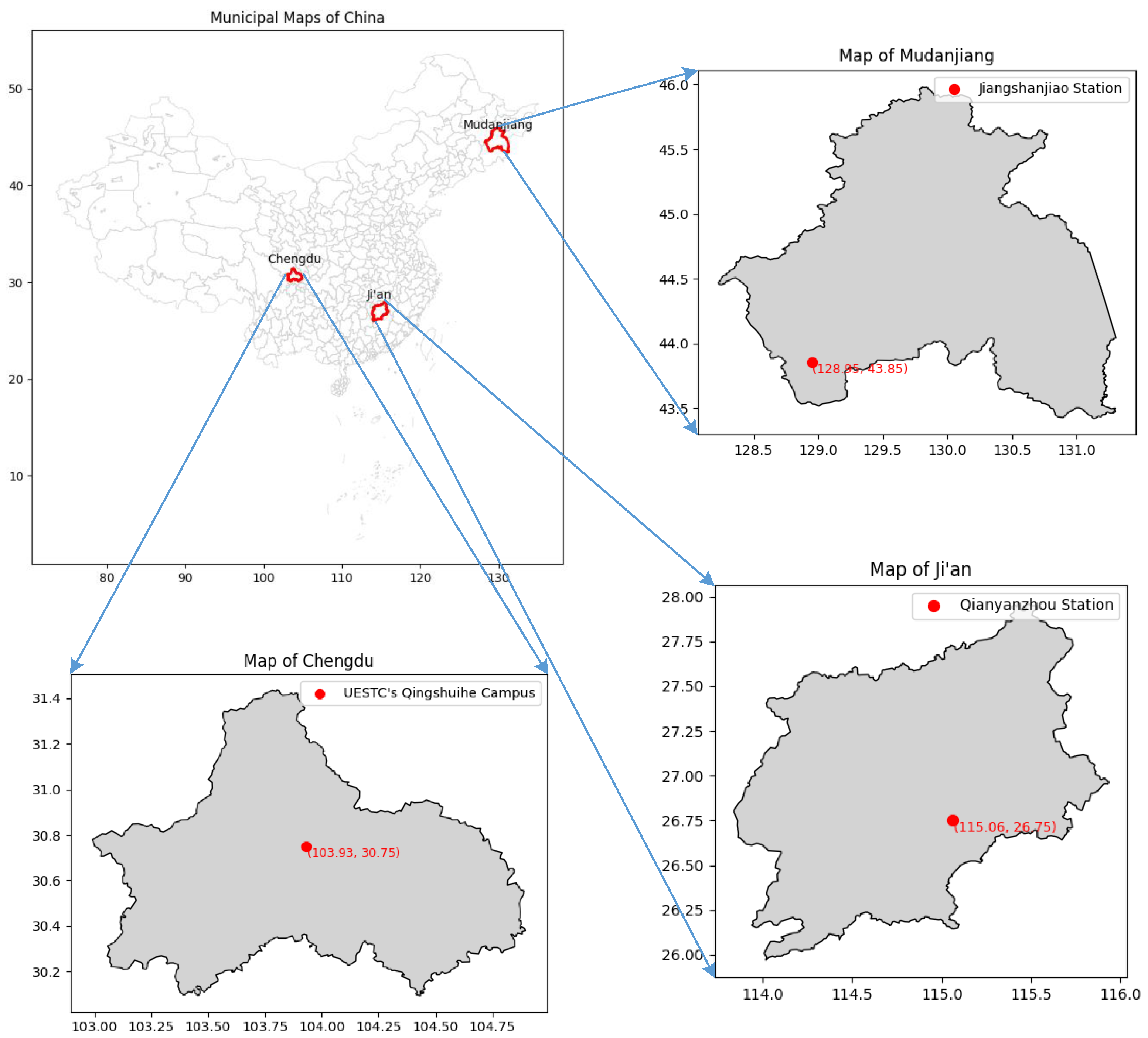
Figure 2.
Experimental data collection. (a)LAI-2200C; (b) LAI-2200C measurement principle; (c) Experimental equipment connection diagram; (d) Experimental site map.
Figure 2.
Experimental data collection. (a)LAI-2200C; (b) LAI-2200C measurement principle; (c) Experimental equipment connection diagram; (d) Experimental site map.
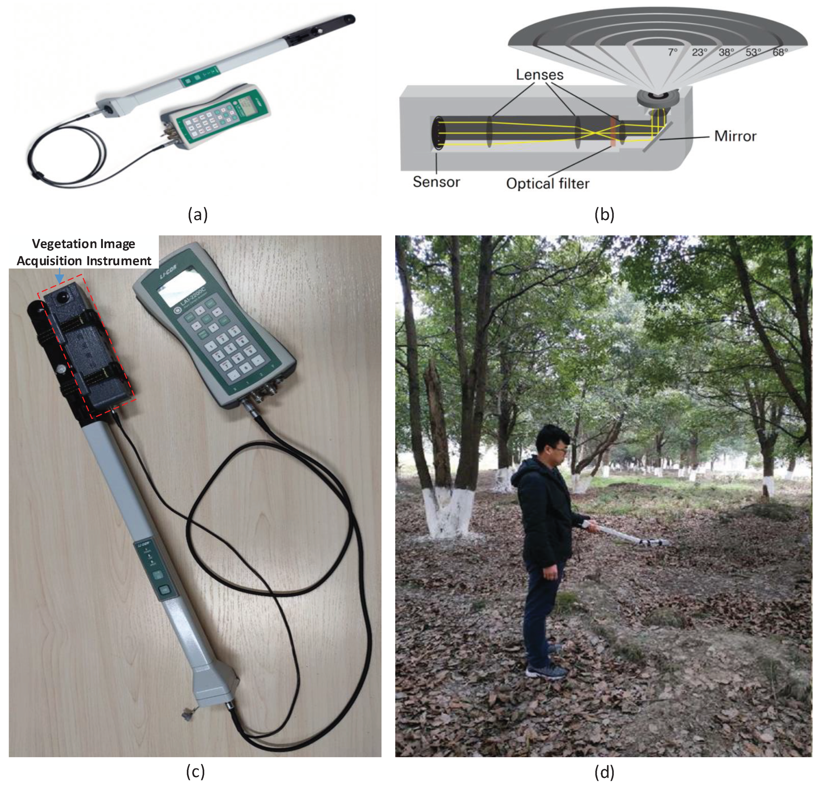
Figure 3.
Schematic diagram of sample point collection.
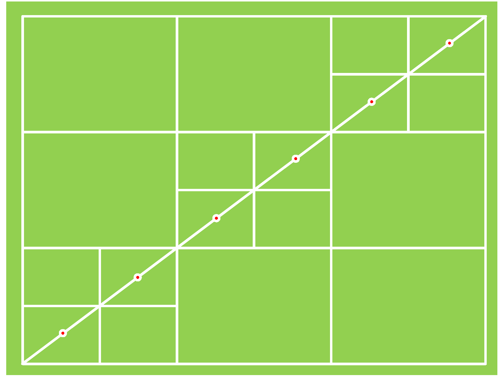
Figure 4.
Sample data example. (a) Sample 1; (b) Sample 2.
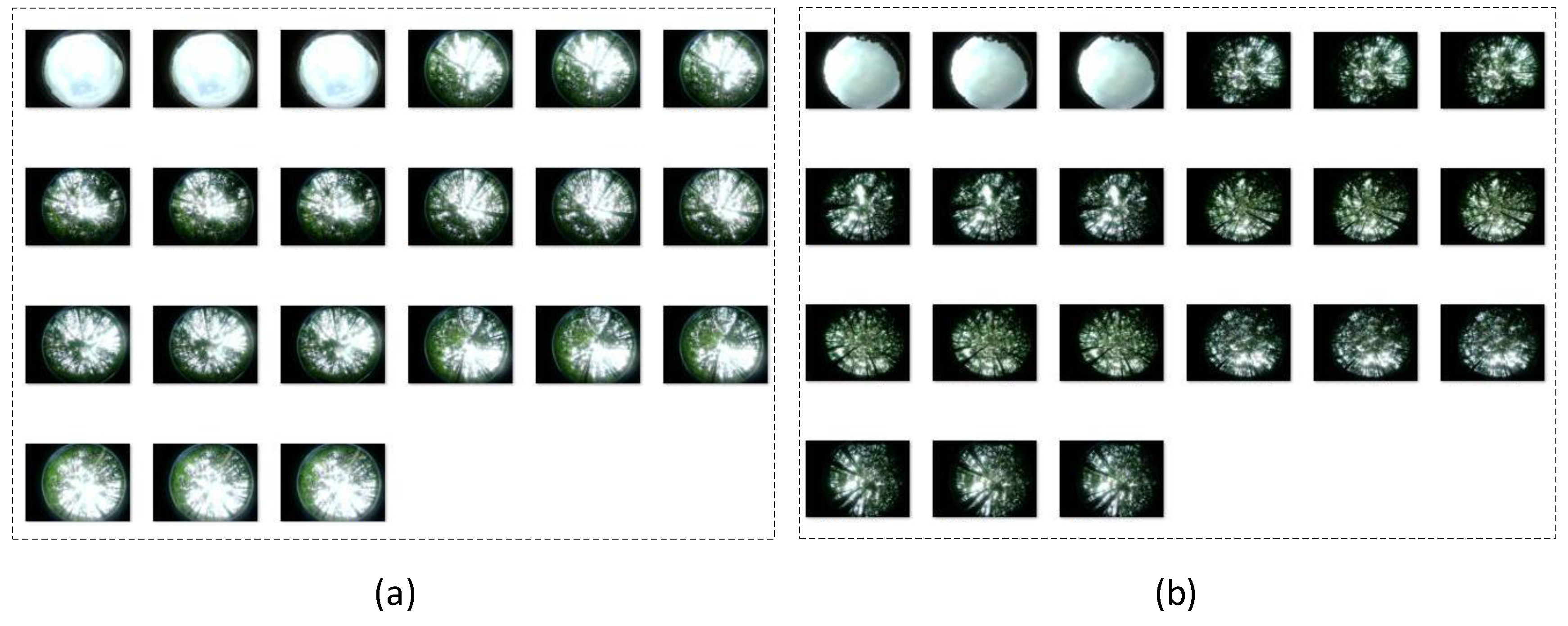
Figure 5.
Schematic diagram of image wavelet decomposition.
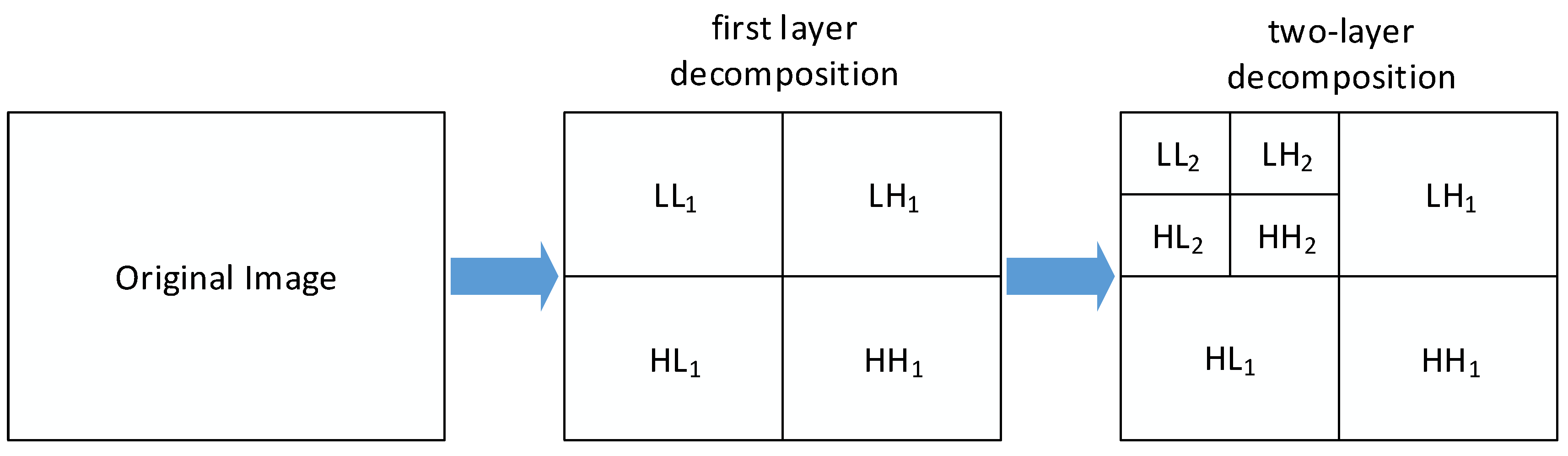
Figure 6.
Image area extraction. (a) Schematic diagram of fisheye lens imaging; (b) Binary image; (c) Imaging area boundary.
Figure 6.
Image area extraction. (a) Schematic diagram of fisheye lens imaging; (b) Binary image; (c) Imaging area boundary.
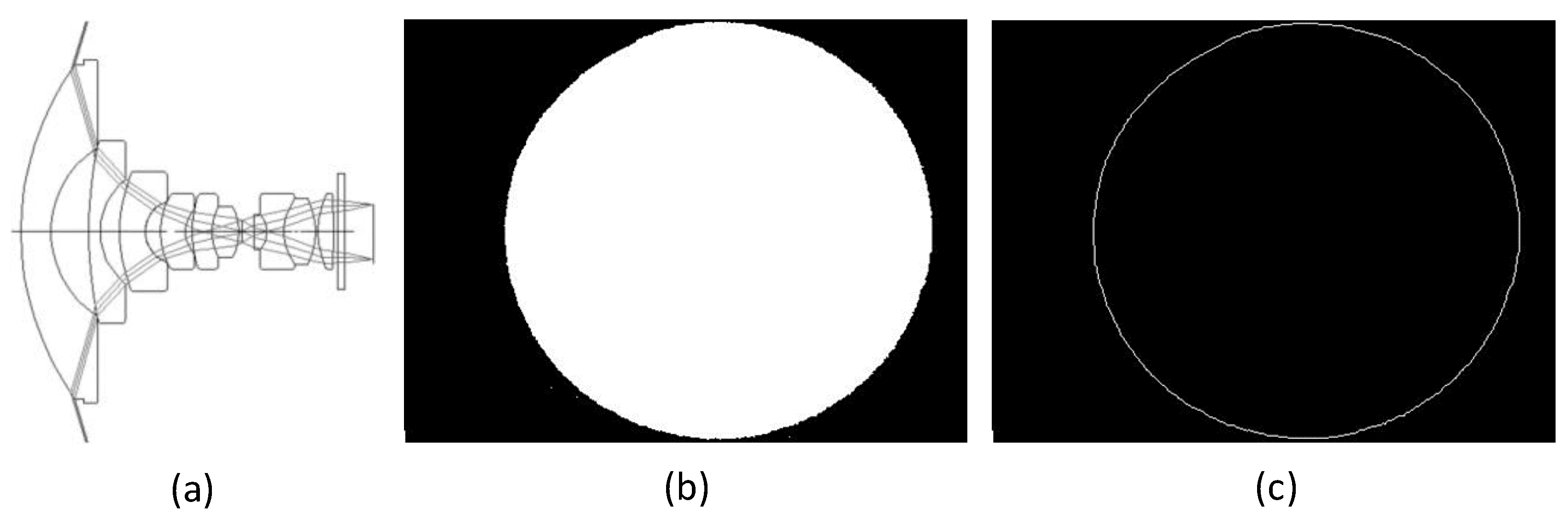
Figure 7.
Wavelet decomposition results. (a) Vegetation canopy image; (b) One layer decomposition result; (c) Second level decomposition results.
Figure 7.
Wavelet decomposition results. (a) Vegetation canopy image; (b) One layer decomposition result; (c) Second level decomposition results.
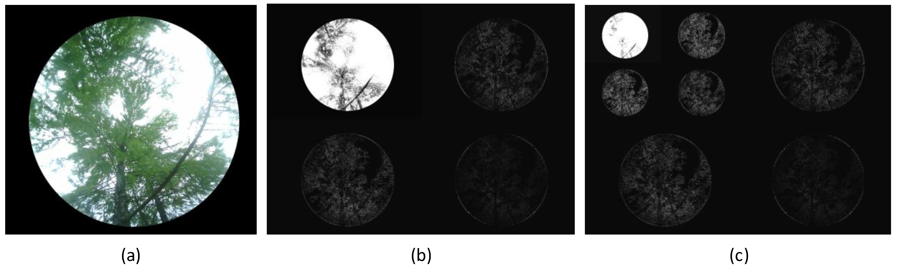
Figure 8.
Fixed coefficient suppression algorithm segmentation results. (a) Original image; (b) reconstructed image; (c) reconstructed image; (d) reconstructed image; Figures (e) to (h) show the Otsu’s method segmentation results of figures (a) to (d).
Figure 8.
Fixed coefficient suppression algorithm segmentation results. (a) Original image; (b) reconstructed image; (c) reconstructed image; (d) reconstructed image; Figures (e) to (h) show the Otsu’s method segmentation results of figures (a) to (d).
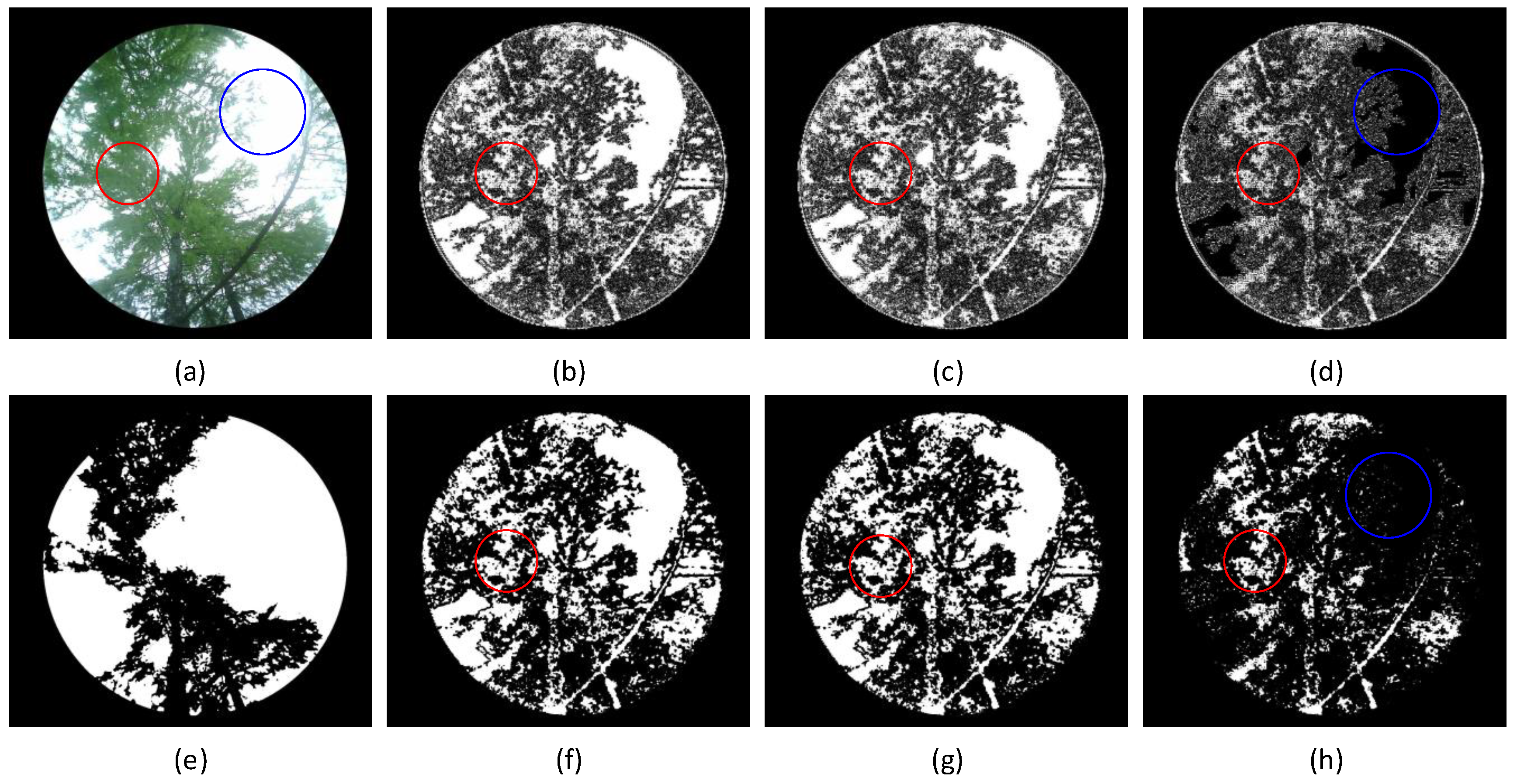
Figure 9.
Grayscale mean-based suppression segmentation results. (a) Original image; (b) reconstructed image; (c) reconstructed image; (d) reconstructed image; Figures (e) to (h) show the Otsu’s method segmentation results of figures (a) to (d).
Figure 9.
Grayscale mean-based suppression segmentation results. (a) Original image; (b) reconstructed image; (c) reconstructed image; (d) reconstructed image; Figures (e) to (h) show the Otsu’s method segmentation results of figures (a) to (d).
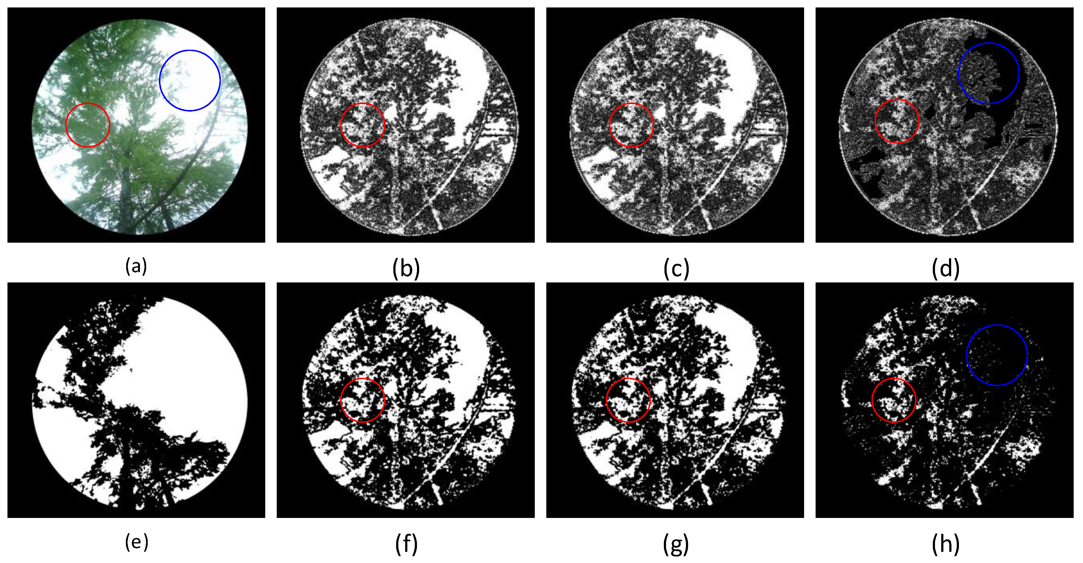
Figure 10.
Dynamic optimization of suppression algorithm process.
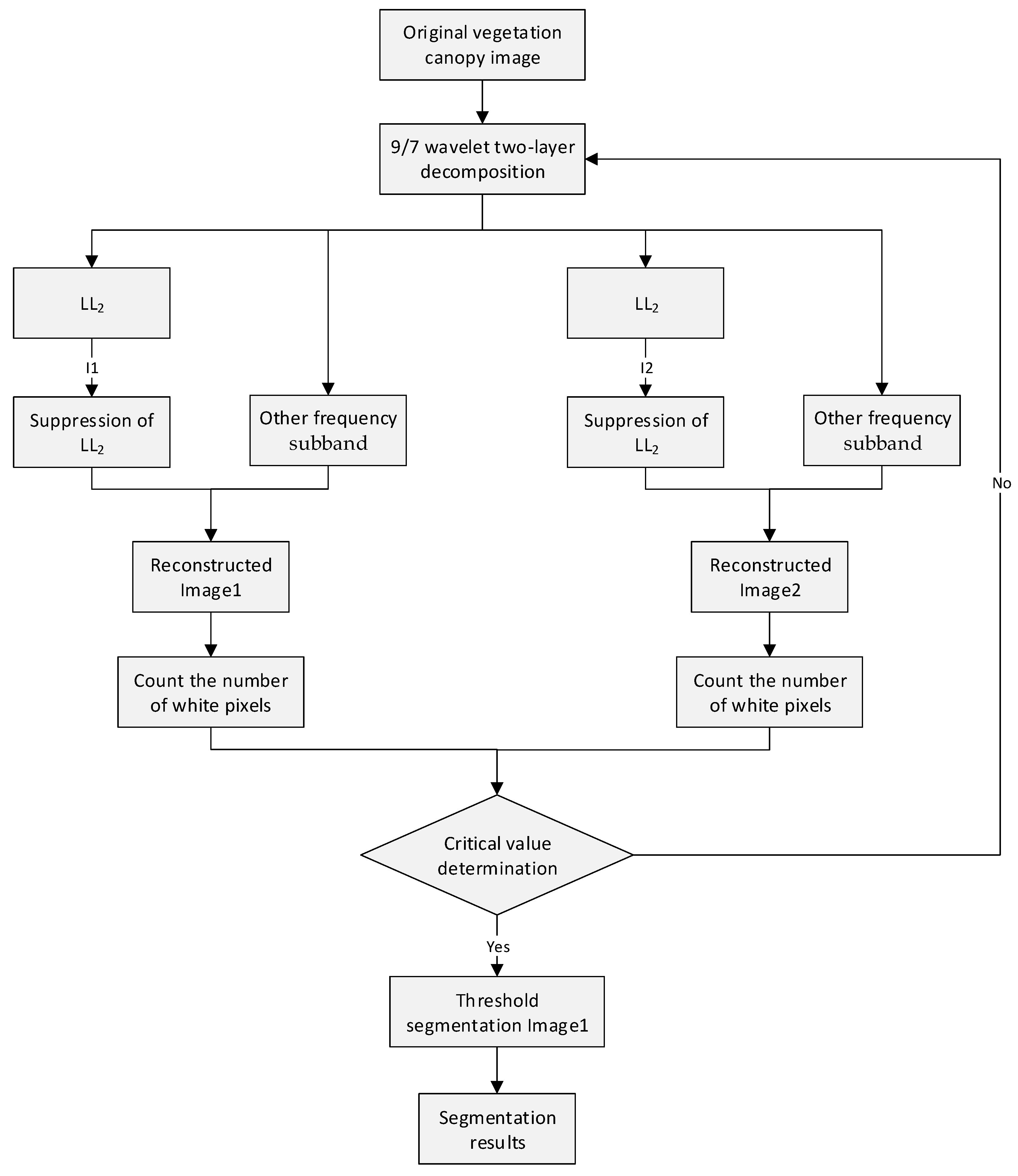
Figure 11.
Results of dynamic optimization suppression method. (a) Original image; (b) Reconstruct image (); (c) Reconstruct image (); (d) The final output image.
Figure 11.
Results of dynamic optimization suppression method. (a) Original image; (b) Reconstruct image (); (c) Reconstruct image (); (d) The final output image.
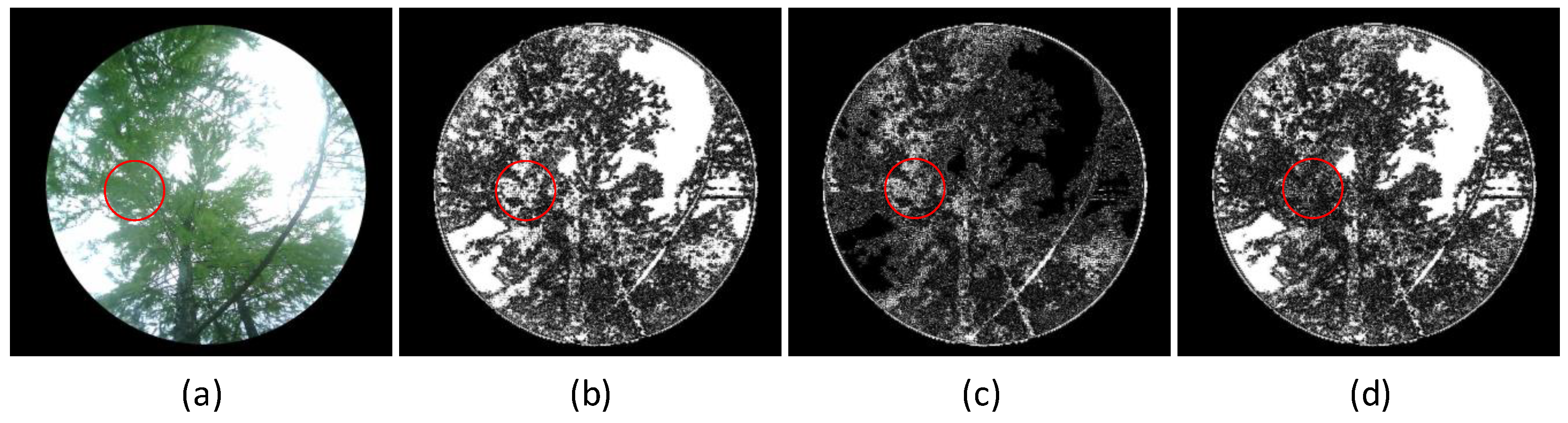
Figure 12.
Comparison of segmentation results. (a) Original vegetation image; (b) Fixed coefficient suppression algorithm (); (c) Grayscale mean-based suppression algorithm (); (d) Dynamic optimization suppression algorithm; figures (e) to (h) show the Otsu’s method segmentation results of figures (a) to (d).
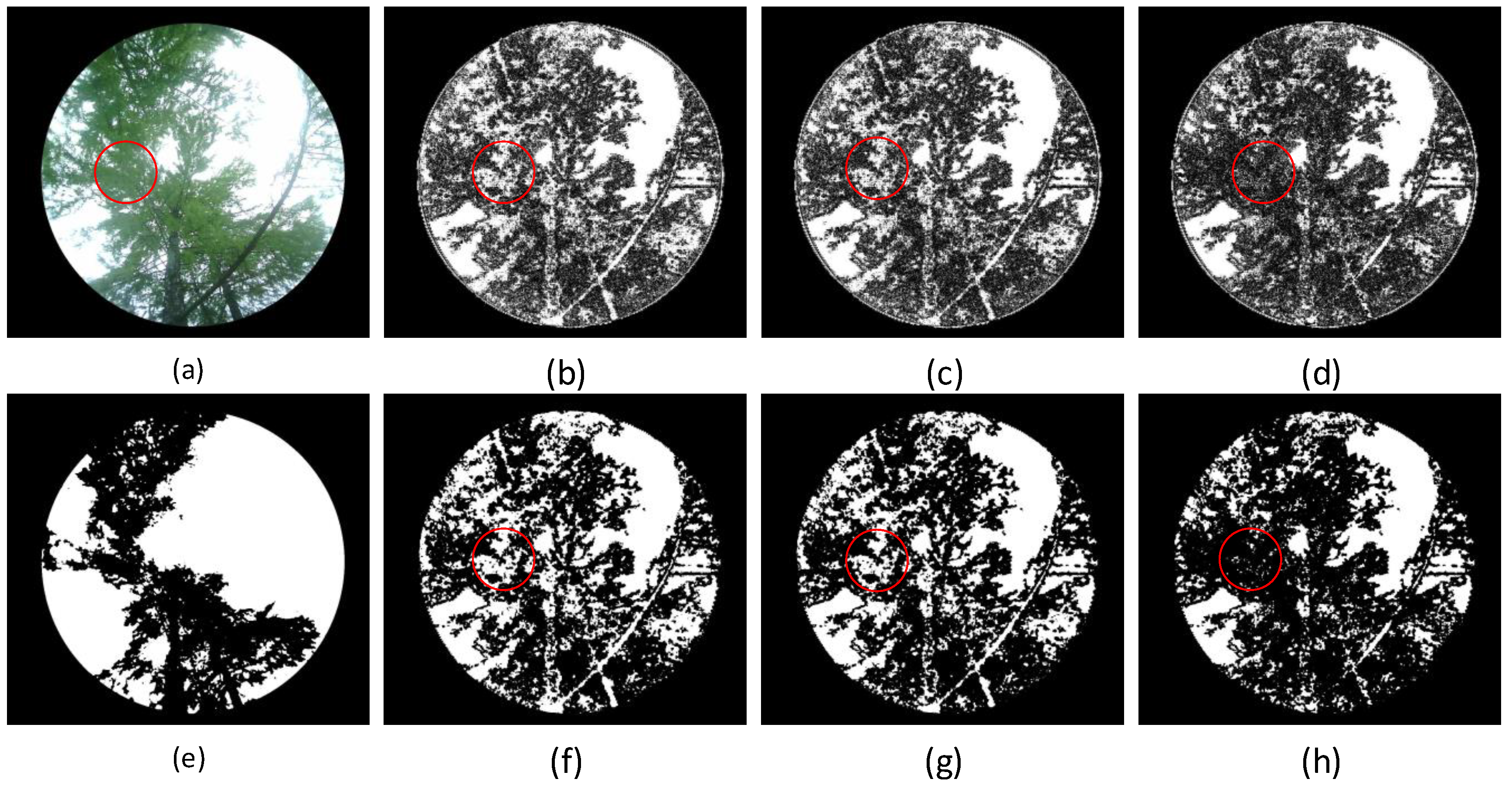
Figure 13.
Correlation analysis of LAI values. (a)Chengdu;(b)Jiangshanjiao;(c)Qianyanzhou;(d)All.
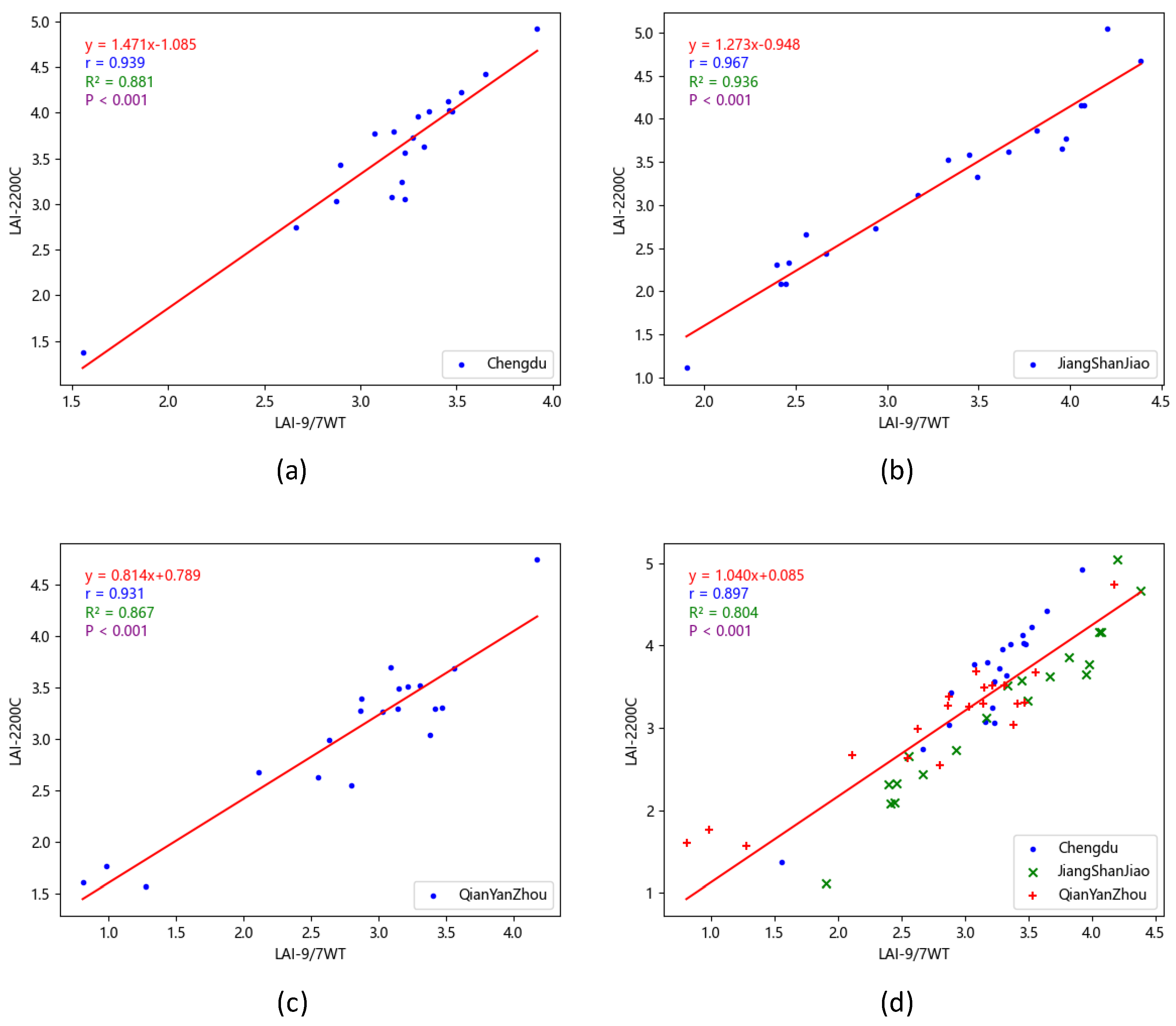
Figure 14.
Boxplot of the LAI value. (a)LAI-2200C;(b)LAI-9/7WT.
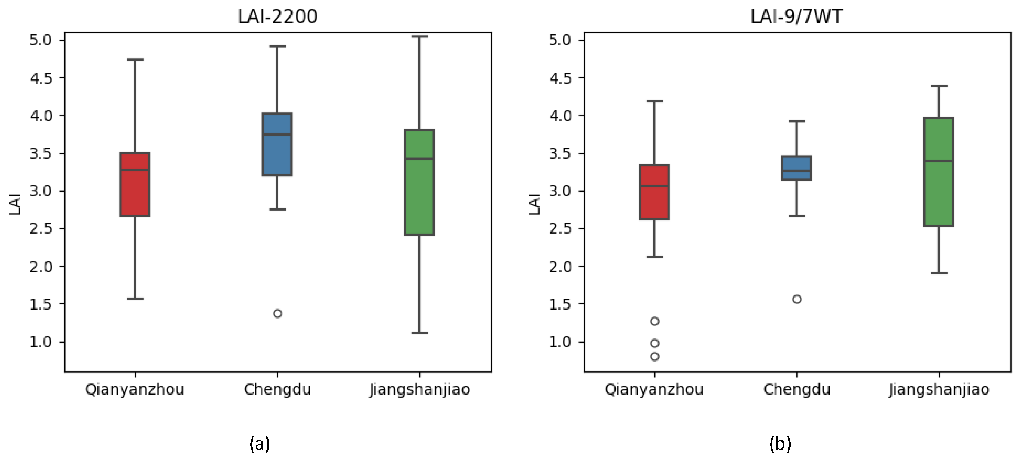
Figure 15.
Image segmentation results. Figures (a) to (d) show the original images; Figures (e) to (h) show the fixed threshold method segmentation results of figures (a) to (d); Figures (i) to (l) show the traditional Otsu’s method segmentation results of figures (a) to (d); Figures (m) to (p) show the improve Otsu’s method segmentation results of figures (a) to (d).
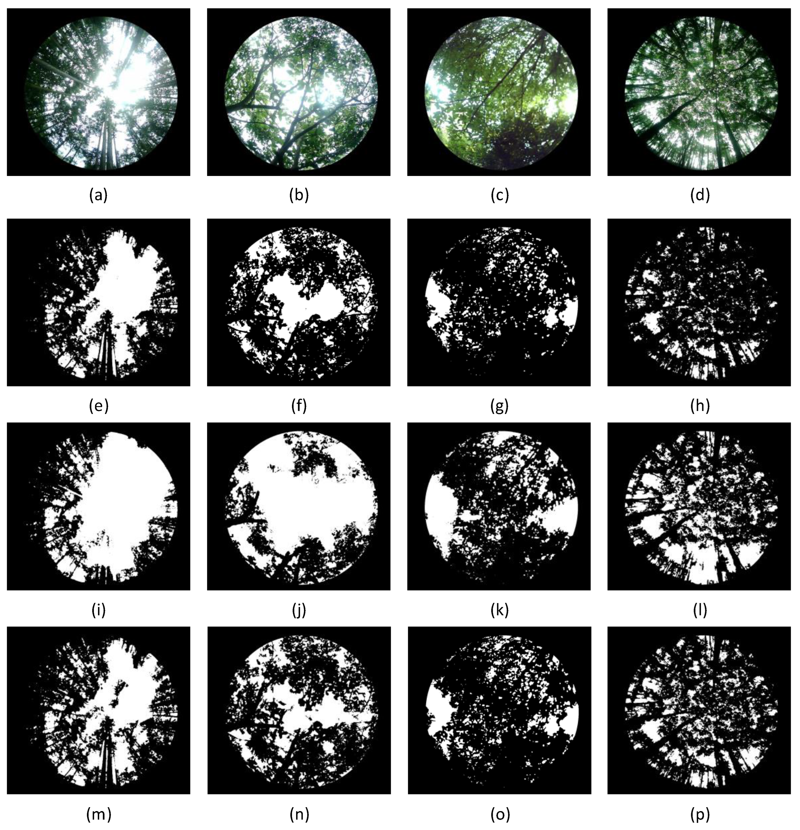
Figure 16.
Dynamic optimization suppression algorithm segmentation results. Figures (a) to (d) show the original images; Figures (e) to (h) show the reconstructing images with wavelet transform of figures (a) to (d); Figures (i) to (l) show the fixed threshold method segmentation results of figures (e) to (h); Figures (m) to (p) show the traditional Otsu’s method segmentation results of figures (e) to (h); Figures (q) to (t) show the improve Otsu’s method segmentation results of figures (e) to (h).
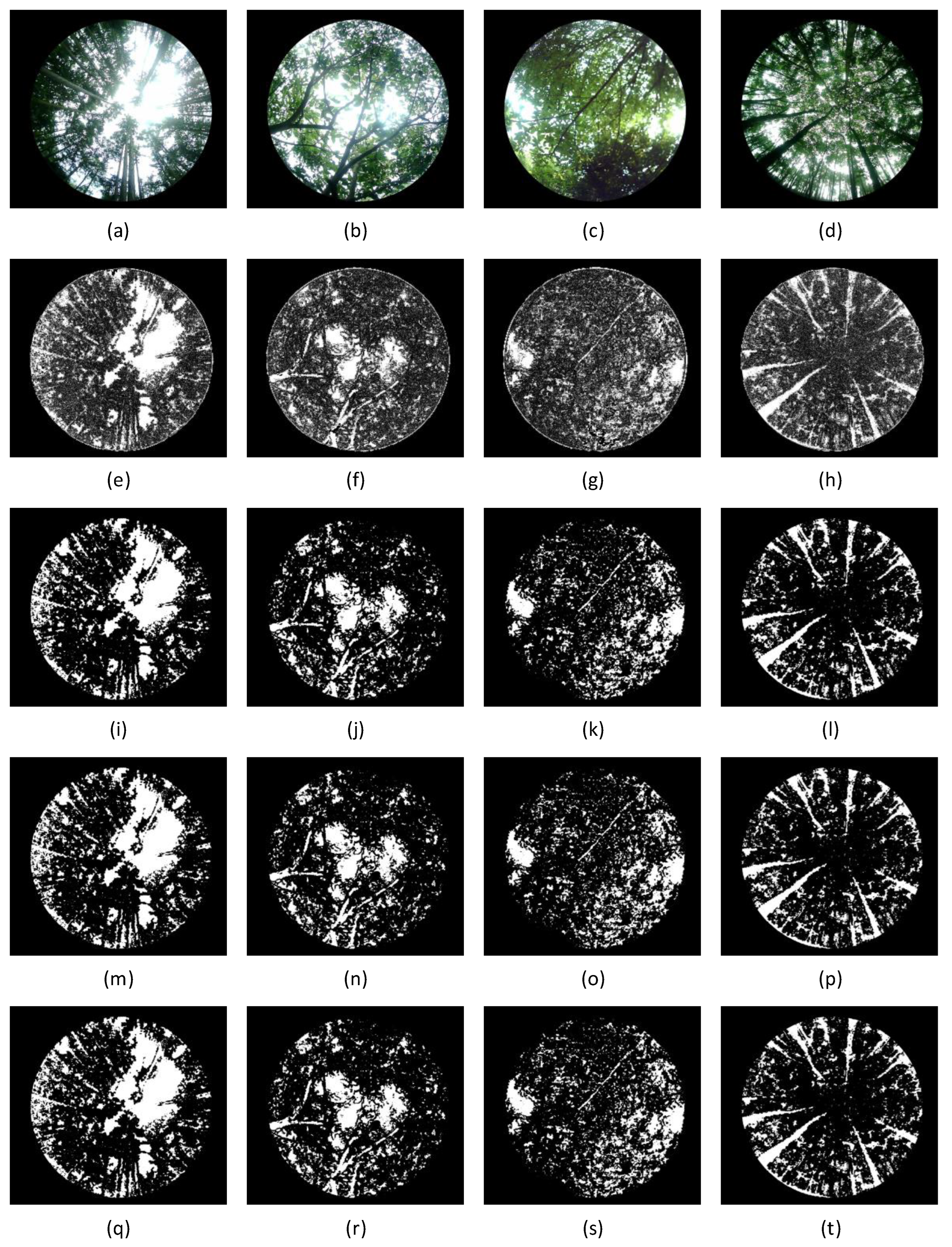

Table 1.
Overview the study area.
| SN | Area name | Vegetation type | Climate type | Landform type |
|---|---|---|---|---|
| 1 | Jiangshanjiao Station, Heilongjiang,China | coniferous and broad- leaved mixed forest | Temperate monsoon climate | Low mountain and hilly landform |
| 2 | Qianyanzhou Station, Jiangxi, China | evergreen broad-leaved forest | Subtropical monsoon climate | Red Soil Hills |
| 3 | Qingshuihe Campus of UESTC,Sichuan,china | evergreen broad-leaved forest | Subtropical monsoon climate | Plain |
Table 2.
Weight Factors.
| 7° | 12.5 | 0.0266 | 0.0427 |
| 23° | 12.5 | 0.0852 | 0.1369 |
| 38° | 12.5 | 0.1343 | 0.2157 |
| 53° | 12.5 | 0.1742 | 0.2798 |
| 68° | 12.5 | 0.2023 | 0.3248 |
Table 3.
Evaluation of Single Sample Reconstruction Results.
| Fixed coefficient suppression algorithm |
Grayscale mean-based suppression algorithm |
Dynamic optimization suppression algorithm |
|||
|---|---|---|---|---|---|
| 0.01 | 0.02 | 0.01g | 0.02g | - | |
| DIR | 0.6077 | 0.6272 | 0.6487 | 0.6663 | 0.7859 |
| Ui | 0.978 | 0.9774 | 0.9799 | 0.9798 | 0.9835 |
| 1.4856 | 1.5141 | 1.3049 | 1.2796 | 0.9549 | |
| 23.6957 | 23.403 | 22.9683 | 22.7328 | 20.9293 | |
| 0.5266 | 0.4819 | 0.4625 | 0.4266 | 0.4256 | |
| 2.638 | 2.6618 | 2.4393 | 2.4062 | 2.2444 | |
Table 4.
Evaluation of Multi-Sample Reconstruction Results.
| Fixed coefficient suppression algorithm |
Grayscale mean-based suppression algorithm |
Dynamic optimization suppression algorithm |
|||
|---|---|---|---|---|---|
| 0.01 | 0.02 | 0.01g | 0.02g | - | |
| DIR | 0.6437 | 0.6537 | 0.6668 | 0.6723 | 0.7481 |
| Ui | 0.9442 | 0.9437 | 0.944 | 0.944 | 0.9589 |
| 2.6149 | 2.6527 | 2.4204 | 2.414 | 2.1597 | |
| 35.2194 | 35.135 | 34.2992 | 34.2531 | 33.1133 | |
| 1.986 | 1.9812 | 1.9371 | 1.9312 | 1.7034 | |
| 2.9535 | 2.9765 | 2.7295 | 2.7167 | 2.4775 | |
Table 5.
Boxplot data sheet of the LAI value.
| Study area | LAI-2200C | Dynamic optimization suppression algorithm | ||
|---|---|---|---|---|
| Chengdu | median | 3.748 | 3.252 | |
| 75th percentile and 25th percentile | 75th percentile | 4.016 | 3.456 | |
| 25th percentile | 3.199 | 3.140 | ||
| Difference | 0.817 | 0.316 | ||
| extremum | maximum | 4.917 | 3.919 | |
| minimum | 1.374 | 1.557 | ||
| Jiangshanjiao | median | 3.425 | 3.391 | |
| 75th percentile and 25th percentile | 75th percentile | 3.792 | 3.961 | |
| 25th percentile | 2.412 | 2.533 | ||
| Difference | 1.38 | 1.428 | ||
| extremum | maximum | 5.040 | 4.387 | |
| minimum | 1.110 | 1.904 | ||
| Qianyanzhou | median | 3.279 | 3.061 | |
| 75th percentile and 25th percentile | 75th percentile | 3.494 | 3.328 | |
| 25th percentile | 2.664 | 2.612 | ||
| Difference | 0.83 | 0.716 | ||
| extremum | maximum | 4.738 | 4.177 | |
| minimum | 1.566 | 0.807 | ||
Table 6.
Analysis of LAI value Error
| Chengdu | Jiangshanjiao | Qianyanzhou | ALL | |
|---|---|---|---|---|
| RMSE | 0.533 | 0.318 | 0.415 | 0.431 |
| MAE | 0.461 | 0.234 | 0.358 | 0.351 |
Disclaimer/Publisher’s Note: The statements, opinions and data contained in all publications are solely those of the individual author(s) and contributor(s) and not of MDPI and/or the editor(s). MDPI and/or the editor(s) disclaim responsibility for any injury to people or property resulting from any ideas, methods, instructions or products referred to in the content. |
© 2025 by the authors. Licensee MDPI, Basel, Switzerland. This article is an open access article distributed under the terms and conditions of the Creative Commons Attribution (CC BY) license (http://creativecommons.org/licenses/by/4.0/).
Copyright: This open access article is published under a Creative Commons CC BY 4.0 license, which permit the free download, distribution, and reuse, provided that the author and preprint are cited in any reuse.


