
Submitted:
06 March 2025
Posted:
07 March 2025
You are already at the latest version
Abstract
Past studies of urbanization in the United States find that college-educated (power) couples migrate to metropolitan areas at higher rates than both educated single persons and other couples with less education. A common explanation is that power couples receive disproportionately high co-location benefits from cities, and therefore migrate to urban areas more than other groups. This study leverages the Public Use Microdata Sets to understand urbanization rates for couples between 2007 and 2022, with a focus on couples attaining degrees beyond the bachelor’s level. The data allows couples to be classified into nine different power status categories based on joint educational attainment, along with categories for their sexual orientation and racial composition. Results from fixed effects logit models reinforce previous work that power couples urbanize at higher rates than otherwise equal peers. Urbanization rates are even stronger for more advanced degree holders generally, though the effect is disproportionately higher for black couples, while it is disproportionately weaker for some same-sex couples. The added nuance of these results provides important insight into migration patterns for local policymakers hoping to better understand shifting demographics across the country, particularly those contending with the effects of `rural brain drain.’
Keywords:
power couples
; urbanization
; rural brain drain
; migration
; racial demographics
; sexual orientation
1. Introduction
The structure and dynamics of urbanization patterns have been popular topics of study in recent decades. Like other countries, many have found the population in the United States demonstrates an increasing trend towards urban environments. Often termed “rural brain drain," past work investigates the phenomenon of highly educated individuals migrating to urban areas and away from rural ones [for some examples [1,2,3,4,5,6,7]]. This pattern of migration engenders concern. Highly educated individuals tend to earn more income than those with less education, which means that migration of the former implies a movement in earnings (and tax revenue) away from departed regions. In the case of prevalent urbanization, the risk is that rural areas, trapped in a vicious cycle of brain drain, will be unable to attract or retain labor market talent and therefore increasingly lag behind urban areas.
Alongside discussions of rural brain drain, Costa and Kahn [8], among others, provide evidence that at least some of this urbanization phenomena can be explained by the co-location desires of highly educated couples. They use U.S. Census data from the decades between 1940 and 1990 to show that the percentage of power couples – partnerships wherein both parties have at least bachelor’s degrees – increased over these years at a rate higher than would be expected from reference groups of highly educated single people. In other words, and as an oversimplification, if many choose to migrate to urban areas for economic and social benefits, there is something unique about being in a couple that provides additional benefits to settling in an urban environment. They term these additional benefits to couples `co-location benefits,’ and estimate their effect on the probability of urbanization by using a triple difference-in-difference approach. While not necessarily their conclusion, the results of Costa and Kahn [8] suggest that one way to prevent increased urban-rural inequality would be to increase work opportunities and amenities that educated couples enjoy in rural areas.
As the percentage of the population that earns a bachelor’s degree (and beyond) in the United States has grown since the Costa and Kahn [8] study, the worry is that migration of the most educated at higher rates might accentuate the effects of brain drain. Given the granularity of recently available data, our primary research question is: do the previously found trends persist when looking specifically at couples that earn even more advanced degrees? To answer this question, we utilize the Public Use Microdata Sets (PUMS) for 2007, 2012, 2017, and 2022 to analyze the probability of urbanization by educational attainment, but with more finite definitions of power status. The assembled data also allows us to simultaneously investigate the extent to which educationally-based migration patterns may differ across demographic groups (e.g. race and sexual orientation). Finally, an auxiliary contribution to our work is that PUMS data are available annually and include a wide range of demographic, economic, and location information for individuals across the country. The hope is that this study models how use of this freely available data can lead to increased dissemination of timely information for policymakers grappling with urbanization trends.
After assembling the data, married individuals are compared with their spouses and categorized by their joint educational attainment (which we term: powerStatus), their sexual orientation (copType), racial composition (raceStatus), and participation in the labor force (laborStatus, which is used to verify results from previous studies). Assigning married individuals to these categories using their individual characteristics allows for a difference-in-difference approach because we use otherwise equal single individuals as points of comparison. To estimate the difference-in-difference models, we employ both fixed effects logit estimation techniques alongside weighted least squares with fixed effects.
Regardless of specification or estimation technique, the results are consistent and robust, with several key conclusions. First, even before the COVID-19 pandemic, the overall rate of urbanization has been decreasing since 2007. At first glance, this may seem to counter many concerns regarding rural brain drain as “work-from-home" options expanded. However, our results also show that the most highly educated couples continue to move to cities at disproportionately higher rates despite this overall trend, which suggests that concerns about rural brain drain’s effects are quite valid. A second key result is that while all couples with high power classification are more likely to live in cities, separating advanced degree holders demonstrates that the rate of urbanization escalates as joint educational attainment rises. This result is stronger when both partners participate in the labor force and is particularly strong for highly educated black couples. On the other hand, highly educated same-sex (male-male) couples were less likely to live in cities, particularly if only one partner had a doctorate or professional degree.
Collectively, this preview of results suggests that co-location benefits do differ across racial and sexual orientation categories. From the perspective of a particular urban area, this demographically-driven result would be important to consider as policymakers look to evaluate local programs and plan for the future demographics of their region. With studies continuing to show the strong, positive link between diversity (both ethnic and intellectual) and economic growth, such an understanding is imperative for good regional policy [9,10,11,12].
The remaining sections of the paper are as follows. Section 2 introduces the most relevant literature for the present analysis, with special attention paid to the literature on migration patterns and urbanization across educational categories. Section 3 describes how our data source differs from previous work and provides some insights into the depth of prospective questions PUMS could address in future work. Section 4 discusses our methodology and econometric approach, given the structure of the PUMS data. Section 5 discusses the results of our empirical estimations, with a focus on power classification even in discussions of the other couple classifications. Section 6 finishes with over-arching conclusions and possibility for future work.
2. Relevant Studies on Migration Patterns and Co-Location Effects
Broadly, studies of urbanization often focus on its general trends, its impacts, or the demographic differences in the rate of urban migration. To underscore the general trends, the percentage of U.S. residents living in urban areas increased from 40% to 80% between 1900 and 2000 [13]. This overall trend of rapid urbanization led to many studies (some of which are cited in other contexts shortly) investigating the effects of this trend. Among these, increased urbanization has been linked with higher economic growth [14,15] and employment growth [16]. Glaeser and Gottlieb [16] (and others) model this relationship via agglomeration effects that increase the flow of ideas and spur innovation.1
Of course, as results show that innovation affects growth rates, studies of the link between educational attainment and urbanization rates became widely examined, especially in the context of “rural brain drain."2 As an inspiration for this study, Costa and Kahn [8] examine the causes of urbanization through the lens of benefits accruing differently to married individuals based on their education level. They coin the term “power couples" – a term we adopt – to refer to couples wherein both partners have a college education. Their theoretical model suggests that these dual, college-educated households receive unique `co-location benefits’ associated with living in metropolitan areas. Indeed, large cities with educated populations give both parties superior career results [18].
To separate power couple urbanization from overall urbanization trends, Costa and Kahn [8] use coincidental power couples – otherwise equal single individuals that could be partners – as a reference group. In other words, they compare urbanization rates for power couples with otherwise equal single peers of equal educational status in a form of difference-in-difference. Frequently, described as triple difference-in-differences analysis, they find that educated individuals move to cities at higher rates than those with less education, and that if two individuals were a member of a power couple, they urbanized at rates above and beyond that of just highly educated individuals. The results of their theoretical model suggest that 35% of power couple urban migration is due to their unique co-location problem. To re-emphasize how this paper links directly to their work, our primary research question is: can we find evidence that the co-location effects are stronger when looking at those with even more advanced degrees? If so, it is likely that previous work that only separates the college-educated from everyone else are likely to understate the potential for rural brain drain to accelerate.
With this in mind, there are several notable studies beyond [8] that are relevant for this work. Each serves as a motivation for our empirical approach and focus on demographic characteristics of migrants. One demographic determinant of migration patterns is age; urban areas appeal to younger, educated workers who value labor market opportunities and city-specific amenities. Consequently, younger people are typically a large portion of migrants to high-growth urban areas [2,19,20,21,22,23]. Evidence supports that the number of prime-age workers (aged 25 to 54) has increased in urban/suburban counties while decreasing in rural ones since 2000 [24]. Of these prime-age individuals, migration patterns also suggest that educated people are particularly drawn to the increasing returns associated with city size [16,25]. By contrast, couples over fifty value locations with high amenities rather than lucrative business environments, no matter their level of education [26]. This reinforces that age is tightly correlated with migration as younger individuals are more likely to migrate.
As previously hinted in the brief introduction of Costa and Kahn [8] already presented, educational attainment is also a key demographic characteristic studied to explain urbanization patterns. A chief sub-focus of this work has centered on the aforementioned rural brain drain, or high net in-migration of the highly educated to metropolitan environments [27]. Perception plays a role in this decision to migrate to urban environments; educated individuals believe staying in rural areas will make finding well-paying jobs with advancement opportunities impossible [28,29]. Waldorf [2] compares the education profile of migrants to that of non-migrants. This analysis confirms that educated individuals disproportionately locate in cities, but the choice of location is affected by the existence of educated people. In other words, a cluster of educated individuals in urban environments serves as a draw for other educated individuals, perhaps exacerbating rural brain drain trends.
Other studies have examined brain drain’s impact rather than its trends. Miller and Collins [30] build a predictive, theoretical model that uncovers the potential economic effects of zero brain drain between 2023 and 2032 for the state of Mississippi. Their model predicts that without brain drain, Mississippi would have 2000 more jobs, 0.2% higher GDP, and 0.1% higher personal income in 2032 than the status quo alternative scenario of continued, current migration rates. A similar predictive analysis reinforces these results [31].
If rural brain drain is itself a concern, it comes as no surprise that studies focusing on the degree of brain drain are a popular area of research. The focus on dual college-educated households in Costa and Kahn [8] falls into this category, since the suggestion of disproportionately high rates of brain drain only serve to increase concern about its effects. The starting point in this shift to the research most related to this study is that economic self-interest is considered the main determinant of migration; individuals move when the net benefit is positive [16,19,32].
Through this lens, co-location is one aspect of benefits and costs considered, since (presumably) households jointly make migration decisions. However, the idea of “joint" migration is open to interpretation. Studies continue to show that highly educated women, for example, root joint migration decisions based on what is best for their partner, which exacerbates career gender inequities [33]. Even so, there is evidence that both partners in a married couple may intentionally pursue migration strategies that are not individually beneficial, but rather ensure the tradeoff between labor and leisure time best matches the ideology of the couple [34]. Becker and Moen [35] describe how dual-career couples “scale back" or employ strategies to reduce their commitment to paid work by not simultaneously pursuing two high-powered careers. However, women are unequally responsible for “scaling back," which creates barriers to career growth. In studies that focus on heterosexual couples, these negative outcomes affect woman more than their male partners because – subconsciously or consciously – couples often prioritize male careers [34,36,37,38,39,40]. These negative effects for female partners tend to be smaller, however, if they are located in an urban environment [41].
Compton and Pollak [42] similarly explore the gender dynamic of power couple migration by looking at the patterns of “part-power" couples – a term used in Costa and Kahn [8] to refer to couples where only one partner possesses a bachelor’s degree. At baseline, Costa and Kahn [8] find that part-power couples urbanize at similar rates to power couples. Compton and Pollak [42] also distinguish their work from the more stringent definition of couples outlined in previous work like Costa and Kahn [8]. To this end, they define “low power" individuals as those with education beyond high school, but without a bachelor’s degree. From these renewed definitions and categories, they separate the migration of part-power couples where the husband has a college degree from those where the wife does for heterosexual couples. They find that the movement of power couples mirrors those of part-power couples where the husband has a college degree. On the other hand, the patterns of low-power couples are the same as those of part-power couples where the wife has a college degree. Simon [18] echoes this conclusion, finding that a husband’s college degree has a larger effect on joint migration decisions in heterosexual couples. That said Simon [18] also find that part-power couples where the wife holds the degree are more likely to urbanize than low-power ones. Their findings are consistent with the larger body of research on joint migration; implying wives are more likely to be `tied’ movers – that is individuals that migrate more for the gain of their partner rather than their own. Often, these tied movers experience negative career effects due to family migration decisions.
This literature review highlights some trends in the existing research landscape on power couples and co-location. First, several studies have explored the dynamics of power couple migration, but few investigate alternative definitions of couple power status. As Section 3 demonstrates, generating more finite categories for couple power status is relatively simple. Second, when more categories of power status are studied, there are some discussions of demographic differences, but more could exist. Finally, when demographics are given primary focus, they tend to be studies of very finite couple types (e.g. academics or physicians), which might prevent generalizations. The wealth of data in the Public Use Microdata Sets allows this study to more fully incorporate numerous definitions of power status and demographic characteristics, without sacrificing generalizability. The results therefore represent an important contribution to a critical field of study, particularly given the migration-based challenges policymakers face due to circumstances like rural brain drain.
3. Data Sources and Construction
To discuss the differential urbanization trends between various demographic groups, we primarily utilize the Public Use Microdata Sets (PUMS). Published annually from the American Community Survey of the Census Bureau, these publicly available data provide detailed variables that capture the characteristics of individuals and households alike. Educational attainment levels, demographic characteristics, and location of individuals across the United States are among the data provided. Furthermore, each year’s data is meant to be representative of the nation as a whole, providing weights for each person in the sample that can be used to generate a comprehensive view of the United States.
We utilize four years worth of PUMS, 3-year or 5-year samples in this paper: 2007, 2012, 2017, and 2022.3 These years coincide with the Economic Census in the United States and represent a range sizable enough to get a sense for urbanization trends. It should also be noted that the choice of these four years is a practical one. Given the size of each year’s data, computational challenges arise as more years are included.4 As a result, our choice is one borne of a combination of symmetry (five year intervals), functionality (a time horizon that can suggest trends and therefore address our research question), and practicality (computing power).
Several variables within each year’s sample are pivotal for our analysis and classification of individuals. Table 1 briefly describes these variables and includes the most consistent naming convention for those variables in a given PUMS data file.
We primarily utilize the person records from PUMS, rather than the household records as this allows us to customize our classification of households. Because of this, our first step is to use the entirety of a year’s person records to separate households into descriptive categories that define their marital status, racial composition, and educational classification. Because it makes the remaining analysis more consistent, the names given to these categories are italicized below. These abbreviated names are easier to display, particularly for the statistical analyses. What is important to note before getting into the details of execution, is that by using these variables from the PUMS data we are able to classify each married couple based on: 1) their joint educational attainment (powerStatus); 2) sexual orientation (copType); and 3) racial composition (raceStatus).
Turning to data construction, for a particular serial number (household identifier), we first look to ascertain marital status of individuals (MAR). Married individuals are termed married only if there is one other married person in the household; all other individuals in the sample are assigned a category of single for simplicity.5 The crux of putting all other individuals into the single category is that these individuals would not make a spousal, joint migration decision.
After marital status is determined, married couples are split from the single individuals to assign demographic identifiers to married couples only. The educational attainment variable (SCHL) identifies the highest level of education completed for each individual. As is standard in the literature, if neither married partner completed school beyond high school (or GED equivalent), couples are categorized as powerLeast. Previous work has also termed these as “noPower" or “low Power" couples. If both individuals earned doctoral or professional degrees, masters degrees, or bachelor’s degrees, then they are placed in categories we call powerMost, powerMore, and power, respectively. As this is a departure from the terminology of Costa and Kahn [8], it is worth noting that each of these categorizations would have been considered a form of a power couple in their work; we are only further decomposing their category. In another extension beyond what is studied in previous work, if both partners attended some college or earned their associate’s degree, we categorize them as powerLow.
Of course, married couples may not have the same level of education, so the remaining couples are categorized based on the partner with the highest level of education. These couples are classified as: partPowerMost – if one partner had a doctoral or professional degree; partPowerMore – if one partner had a master’s degree; partPower – if one partner had a bachelor’s degree; and partPowerLow – one partner had some education beyond high school.
For other demographics characteristics of couples, copType is an identifier for the sexual orientation of couples, which could be female-female (FF), female-male (FM), or male-male (MM). Finally, each individuals racial category (RAC1P) helps classify couples as asian, (i.e. both partners are Asian), black, or white. If each partner has a different racial category, they are coded as mixed, with other representing all other couple types. The choice to limit the possible values for raceStatus was not made lightly; however Section 5 demonstrates that the sheer quantity of categories decreases the chance of easily interpretable results. We acknowledge this limitation and focus only on the four most concrete categorizations (asian, black, mixed, and white). A more comprehensive investigation of racial categorization is a ripe area for future research.
Even with the necessary reduction in possible categories for raceStatus, there are many demographic identifiers for each married couple. Table 2 provides a visual way to intuit how these categories are constructed. One additional categorization is added for the labor force status (laborStatus) of married couples. This particular measure uses the household records in PUMS, which feature two possible variables to express whether both partners are actively in the labor force (bothLF), one is in the labor force (oneLF), or neither is in the labor force (noLF).
This addition is made on the basis of previous work, like that of Costa and Kahn [8], that shows co-location effects may be stronger for dual-income households. When focusing on dual-income households, we also consider the occupation of each individual. PUMS provides occupational codes for each worker (OCCP) that are too numerous to succinctly list in this paper. However, for two spouses that work, the type of job they perform is likely collinear with the probability of living in an urban environment (e.g. farmers don’t often migrate to urban areas). For this reason, it is worth mentioning here that occupational indicators are a part of the data constructed. Each occupation within OCCP is initiated with a three digit tag that groups related occupations together. For example, `MED’ serves as a common preface to all medical occupations while ’BUS’ tags common business occupations. These tags are stored to the variable jobTag in our dataset to serve as occupation-specific migration effects when studying dual-income couples.
Once household characteristics are determined, the final step to assemble our data is to use the provided state and Public Use Microdata Area (PUMA) information for each person to classify them as living in an urban environment or not.6 Because PUMAs are delineated by population, a PUMA may cover a significant area of primarily rural towns, or several PUMAS may comprise one metropolitan area. Because PUMAs are not neatly defined as urban or rural, we utilize a PUMA to Metropolitan Statistical Area (MSA) “crosswalk" from the Geocorr program of the Missouri Census Data Center (MCDC) [43]. This program provides customizable methods to convert one regional unit to another and, most importantly for this paper, provides estimates of the degree to which areas are urban or rural. For example, DeKalb County, Georgia – a populous, urban county that features Emory University – has an urban proportion of 0.989, which effectively means that 98.9% of the PUMA could be considered urban. By contrast, Newton County – the home of the Oxford College campus of Emory University – has an urban proportion of 0.763. This region has been growing and is close geographically to DeKalb County, but is decidedly more suburban in nature.
We believe this provided urban proportion (which we term, urbPro) to be the most accurate for our analysis because it allows for a spectrum of urban-ness. However, some may be accustomed to a more binary definition of urban or rural. For the binary definition, we assign a status of urban to PUMAs that that are at least 70% urban according to the MCDC urban proportion measure. This forms a binary variable (urb) that takes on a value of one for urban areas and zero otherwise.7 Section 5 will show that while the magnitude of estimated coefficients changes between urbPro and urb as the definition of urban, the results are largely consistent.
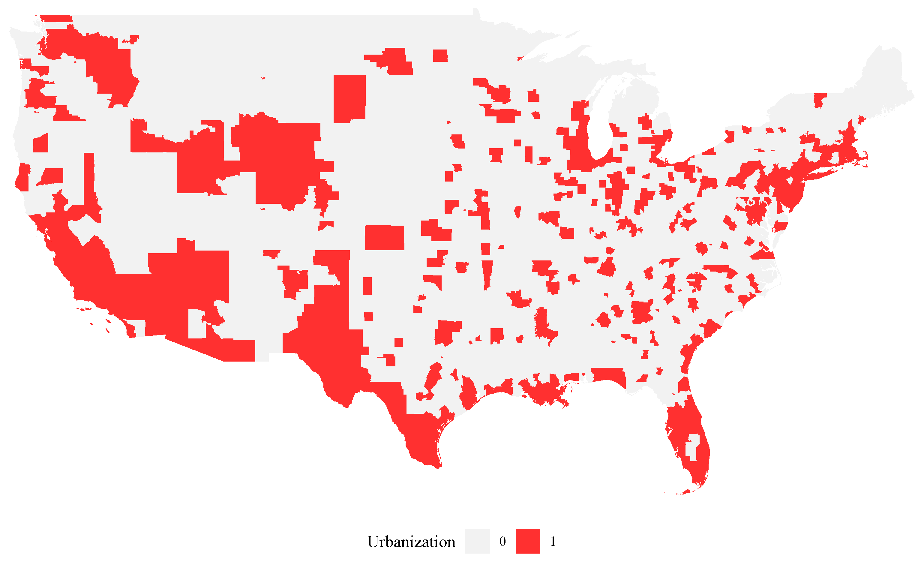
Figure 1 displays two maps of urbanization status for our sample in the year 2022. Not surprisingly, the urbanization definition that allows for urbanization proportions displays a spectrum of urbanization across the United States. Areas of the north and midwest appear to have the lowest urbanization proportions, with population hubs in the expected areas of California, New York, Texas, and Florida. Figure 1b displays the binary definition of urb and provides an example for why the proportion-based measure urbPro is more compelling. Using a binary definition, there are a number of “pockets" of urban areas along the Eastern seaboard. However, someone living adjacent to these areas likely reaps at least some of the benefits of proximity. No matter where our cutoff point to determine urban status, this issue of not capturing partial benefits to those just outside an urban area will always be an issue. It is for this reason that we argue urbanization proportions best capture how we should define urban status.
Figure 1a.
Urbanization Proportion (urbPro)
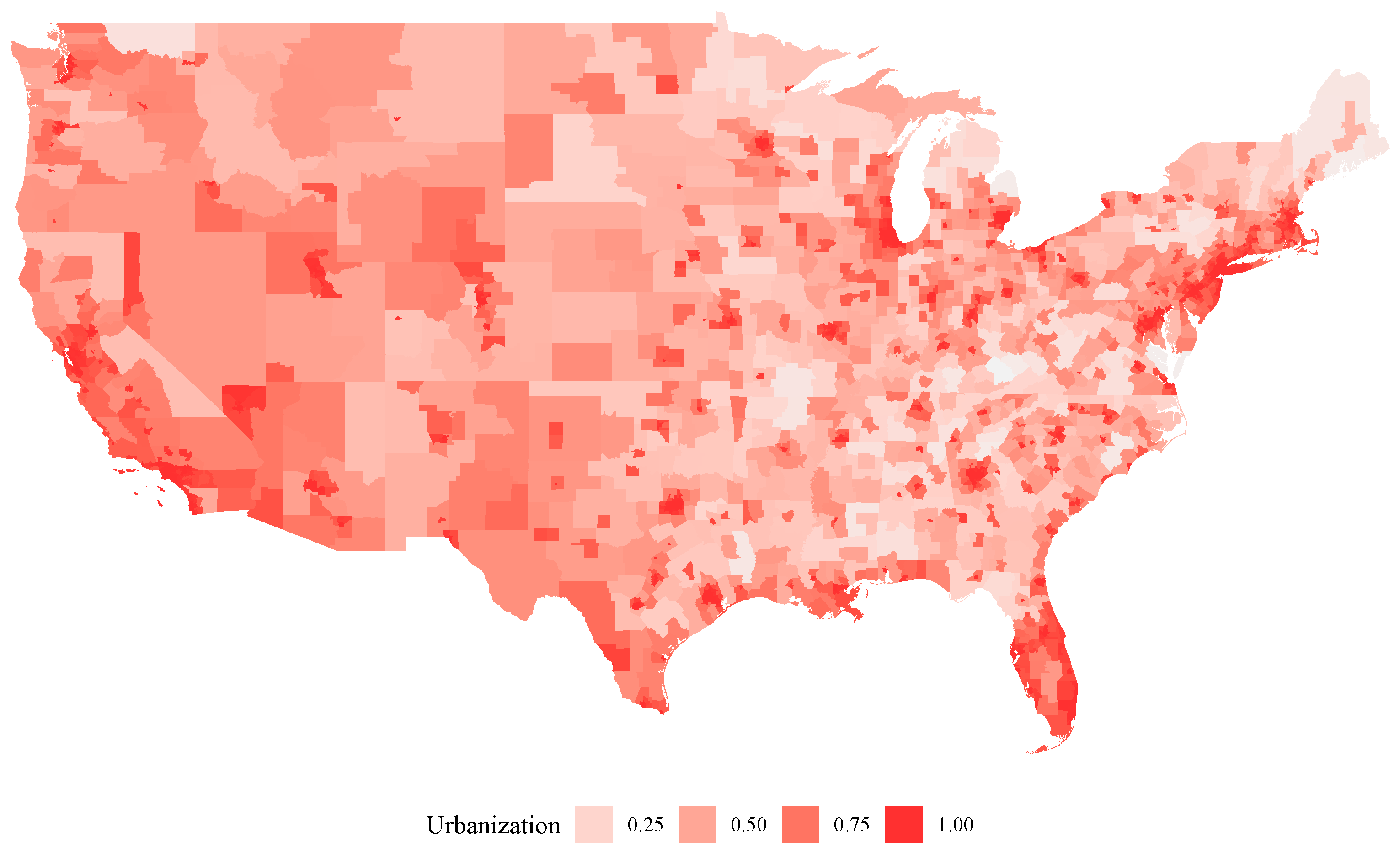
Figure 1b.
Urbanization - Binary Definition (urb)
3.1. Summary Statistics of Key Data
Based on these definitions of urban areas, Table 3, Table 4, Table 5 provide select summary statistics across power status, sexual orientation, and couple racial composition, respectively. For each table, we utilize the psych package in R [44] to group summary statistics across the categories. So long as the mean urbanization rate differs along the provided categories, the inclusion of each would be necessary in any statistical estimation that tries to understand whether power couples with different characteristics urbanize in a manner unique to otherwise equal, single peers. In Table 3, Table 4, Table 5, the variable urb represents the binary definition of 70% urban-ness (as defined by the MCDC) already mentioned. The standard deviations (in parentheses below the mean estimates for each year) are naturally higher for this measure of urbanization because the variable can only take on the values of zero or one, which makes the spread of the data seem larger than under the urbPro definition that allows regions to be partially urban and rural simultaneously. urbPro is simply the MCDC-provided measure of urban-ness for each region with no adjustments made.
Several elements from Table 3 are worthy of note. The most obvious is that we only include summary statistics for four groups that best help justify our extension relative to past literature.8 powerLeast is the category tag granted to couples wherein both partners have no more than a high school education; power is the tag for couples that have a bachelor’s degree but no higher, in a manner similar to past studies; and powerMost is the tag for couples wherein both individuals of a couple have doctoral or professional degrees. From these results, we see a clear increase in mean urbanization rates as couples become more educated. Within the sample, if two married partners each had doctoral or professional degrees in 2007, approximately 88% of them lived in urban areas. This rate far exceeds the approximately 63% and 81% of couples that lived in urban areas if they mutually had no more than a high school (or equivalent) or bachelor’s degree education, respectively. This pattern is consistent across years, implying that more educated couples tend to urbanize at higher rates.
That said, Table 3 also shows that regardless of education categorization, the rate of urbanization has decreased since 2007. An initial rationale behind this may be the increased prevalence of work-from-home options post-pandemic, however it remains unclear whether these changes to work structure are transient or permanent. According to the PUMS data collected, 15.2% of all workers worked from home in 2022, up from 5.4% in 2017. The majority of this increase unsurprisingly came in 2020, since only 7.3% worked from home in that year (understated due to when the data was collected) and this number jumped to 17.9% in 2021. These work-from-home rates have declined each year since 2021 [45]. This is interesting to note, but the exact reason behind this phenomena is beyond the scope of this work and research question, so the specific causes for this decline are left to future studies. What is clear from Table 3 is the consistency in higher urbanization rates for higher powerStatus couples.
Turning to summary statistics of copType, Table 4 displays urbanization rates for heterosexual and same-sex couples. Here again there appears to be a subtle decline in urbanization rates after 2017 for all couples. However urbanization rates for same-sex couples began declining in 2012. Across groups, same-sex couples lived in urban areas at far higher rates than their heterosexual counterparts. This remains true across all years in the sample.
Finally, turning to racial composition of couples, Table 5 provides summary statistics for urbanization rates across the categorizations of raceStatus. As with the other summary tables, urbanization rates decline for all racial categories in 2022. Still, asian couples exhibited a far higher probability of living in urban areas that other racial categories while white couples lived in urban areas far less frequently. The difference between asian and white urbanization rates is particularly striking given that the spread between the two is akin to how much more likely power couples are to live in urban environments than powerLeast couples.
Across the provided tables, there appears to be strong evidence that explaining urbanization rates requires the inclusion of powerStatus, copType, and raceStatus as categories due to the stark differences in urbanization rates between groups. Indeed, ANOVA tests (performed offline, available upon request) for the difference in mean urbanization rates across all categories are statistically significant. All told, this provides a compelling reason to include each category constructed in our analysis.
4. Methods Used to Analyze Differential Urbanization Rates
This study leverages the information on individuals (from PUMS) and on couples (constructed) to perform a form of difference-in-difference analysis. This methodology has been commonly utilized, including in the two works most closely related to this present work: Costa and Kahn [8] and Compton and Pollak [42].
In this simple model of urbanization rates, consider individual i, living in location j, in year t. U is an indicator of whether the individual lives in an urban location, and is therefore primarily a function of j.9 From Section 3, U could be measured as either urbPro – indicating the degree of urban-ness for that particular individual’s location – or urb – the binary construction of urban described above. Previous research suggests that the choice to live in an urban environment could stem from some combination of economic opportunity, social prospects, urban amenities available, and/or co-location benefits – each of which could accrue to any individual i, though only co-location benefits accrue to those in a couple. The individual’s choice of location j, and by extension the degree of urban environment, could then be expressed in the baseline model of Equation (1).
In Equation (1), an individual’s characteristics might place them in a couple group, depending on whether they are married or not. captures the demographics of an individual and can best be understood as a vector of age, educational attainment levels, sex, and race, all of which might affect one’s urbanization status. The effects of individualized demographics on urbanization is therefore represented by .
represents a vector of indicators of the couple status for each individual. Each non-married PUMS respondent is given a value of single for powerStatus, copType, and raceStatus. By assigning a common status of single for all non-married persons in the sample, remaining coefficients attached to powerStatus, copType and raceStatus are captured in as differential urbanization effects for members of these groups relative to their single peers. is therefore a vector of our primary coefficients of interest.
Finally, it is clear that urbanization rates differed over time in the summary statistics. Likewise, geography factors into the potential for someone to live in an urban environment (i.e. rural states like Wyoming have few urban living options). and represent location (state and PUMA) and year fixed effects to capture location- and time-based trends in urbanization. is the error term for each individual.
With this estimating equation construction, it becomes clear how the coefficient can be interpreted as a difference-in-difference estimator. It captures how couples urbanize differently from singles with the same characteristics, with the inclusion of couple-based demographic identifiers in allowing for differences between couple groups.
If Equation (1) represents the primary estimating function, we also estimate models that explicitly include laborStatus in order to see if dual-income couples urbanize differently. Equation (2) tweaks Equation (1) in a subtle, but meaningful way. In these estimations, a new fixed effect of is included to capture occupational-specific urbanization rate effects. For this, we use jobTag as described previously. When estimating this expression, the primary interest is to understand migration decisions for individuals in the workforce, so the sample is stratified to contain only those with a reported occupation (single or otherwise) and for couples with a laborStatus of bothLF (both in the labor force). This specification captures whether work-oriented couples differ from work-oriented single individuals.
In cases where fixed effects are used, it is often helpful to visualize the extent to which these fixed effects matter.
4.1. Estimation Technique
We estimate Equations (1) and (2) using the fixest package in R [46]. This package provides robust testing and implementation of a variety of fixed effects models. Chief among its features, it allows for clustering of standard errors and weights of observations (which is necessary when using the PUMS data). Across all reported models, observations are weighted using the provided person weights in PUMS and standard errors are clustered according to powerStatus. Alternative choices for clustering did not alter the significance of estimated coefficients.
Given that the dependent variable is bound between 0 (completely rural) and 1 (completely urban), even in cases when urbPro is used, binomial logit models are our preferred estimates. For robustness, we also provide several estimates for weighted least squares models in the first set of results. However, after noting their similarity, we only present remaining results from logit models that are better suited for the constructed dependent variable.
Attempting to capture powerStatus, copType, and raceStatus simultaneously is nearly impossible given the implied challenges of coefficient interpretation. Instead, the first models do not consider copType nor raceStatus and instead only focus on the differential urbanization rates by powerStatus. Of course, individual age, sex, and race are included as controls. After estimating models with the whole sample, we include several specifications that focus on workers specifically, subsetting the sample so that laborStatus for couples is bothLF and all single workers have a reported occupation. These estimates might more accurately express co-location benefits for couples, operating on the assumption that dual-income couples require employment to pay their bills in the same way single individuals do (i.e. this comparison removes any effect that cities may have on location decisions made purely for employment reasons).
As the other demographics are included, we stratify the data based on each category of couple (keeping single individuals intact) so that the impact of powerStatus can be compared across estimations. In other words, to account for copType, unique regressions are estimated for each of the categories within this demographic-based couple designation – one for FF couples, one for FM couples, and one for MM couples. The same process is executed for raceStatus, with each stratified sample focusing on a particular couple racial composition in comparison to otherwise equal single peers.
The following section discusses the results of these models and includes comments throughout before our discussion and conclusions.
5. Fixed Effects Results from Logit and Weighted Least Squares Models
To facilitate the dissemination of results, this section is divided into subsections that focus on results for powerStatus, copType, and raceStatus, respectively.
5.1. Results for powerStatus Designations
Table 6 provides results for urbanization probability with respect to powerStatus. The coefficients on controls (e.g. age, individual race, etc.) are not reported to remain focused on the primary results. They are available upon request for this and future regression tables.
The first four columns of Table 6 display weighted least squares (WLS) and binomial logit (Logit) estimates for each version of urban-ness definition. The preferred specification is column (2), which suggests that power couples (those that jointly have a bachelor’s degree) are 5.1% more likely to live in an urban environment relative to their otherwise equal single peers. Given the primary research question of this study was to ascertain whether this probability rises for more highly educated couple pairings, the answer is clearly yes. powerMost status for a couple is associated with a 15.8% increased probability of living in an urban area. The magnitude of this difference is striking, but underscores why concern over rural brain drain is so high. These couples are likely the highest earners in their respective labor markets and are qualified for skilled work, but disproportionately locate in cities.
The signs and significance of results are consistent for the binary definition of urban-ness (urb). The magnitude of coefficients is expectedly higher, given the standard deviation of this variable being higher. Given our preference for urbPro as the dependent variable and consistent of sign between the two, future tables presented only include results for this definition.
Another interesting result across all specifications is that all forms of partPower couples (partPowerLow, etc.) are statistically less likely to live in urban environments than their otherwise equal, single peers. In general, they were more likely to live in urban environments when compared with powerLeast couples – or those for which neither partner had more than a high school education. This suggests that previous work may overstate the degree to which partPower couples urbanize.
Finally, columns (5) and (6) subset the sample used for estimation to only single status individuals that are working, and couples that are assigned a bothLF for laborStatus. To restate, the coefficients for these models may best reflect non-economic reasons for moving, and therefore capture co-location effects more clearly. In the preferred specification from column (5), powerMost couples that are dual-income earners are about 13.8% more likely to live in urban environments than their single peers. Most interestingly, all coefficients for power or through powerMore become insignificant, which suggests that much of the result from column (2) was actually driven by job opportunities.
5.2. Results for powerStatus Designations, Stratified by Sexual Orientation (copType)
With a sense for the baseline results stemming from powerStatus, the following results stratify the sample by copType. The results would indicate the extent to which couples of different sexual orientations urbanize differently from the average couple of the same educational attainment level. As such, utilizing columns (2) and (5) from Table 6 becomes essential for interpreting the results, which are displayed in Table 7.
Looking at the first three columns from Table 7, some common patterns emerge from the results of Table 6. First, power status couples still tend to live in urban areas at disproportionately higher rates relative to single peers. Beyond that, the variance in results is striking as compared to the baseline powerStatus models, regardless of whether or not occupations and labor force status are considered.
For example, there is no longer consistency of coefficient sign on powerLeast status. FF and FM couples with this status are less likely to live in urban areas much like the baseline results from Table 6. On the other hand, MM couples with powerLeast were more likely to live in urban environments. Similar variance in the sign of the results for partPower designations (beyond power) exist across the categories for couple sexual orientation. Without more investigation, our results could not speak to why this is the case, but these results provide initial evidence of the importance of including demographic characteristics more thoroughly in analysis. Simply put, different demographic groups urbanize at unique rates, regardless of education level.
What also becomes clearer due to the juxtaposition of results is that the coefficients (probability of living in an urban area) all decrease when laborStatus and occupation are considered. This reinforces the suspicion mentioned previously that job opportunities (and by extension, where jobs are located) may be driving many co-location decisions rather than through the co-location benefits described in past work. When controlling for laborStatus, as in columns (4) through (6) some consistency in results across groups re-emerges, though nuances remain. For example, power and powerLow status couples appear less likely to live in urban environments than peers, but this is consistent across each sexual orientation. FF couples are more likely to live in cities after controlling for occupation, while FM and MM couples are less likely to do so. For same-sex, partPowerMost couples, whether FF or MM, urbanization probability was lower.
Another interesting result from Table 7 is that almost every coefficient is statistically significant. This provides evidence that copType – or sexual orientation for couples – is an important feature of migration choices. This may hardly be surprising when considering the political tendencies of rural versus urban areas in the United States. However, each regression contains state and PUMA-level fixed effects that would control for the unobserved (explicitly) features of that region. Coupled with a high implied coefficient that suggests this model has strong explanatory power, the story of politics may not be so simple. For this reason, we argue that Table 7 stresses the importance of considering couple composition in future work that investigates migration decisions. Explaining these urbanization rate differences, particularly after controlling for employment status would shed light on the other factors that induce couples to migrate in differently from single peers.
5.3. Results for powerStatus Designations, Stratified by Couple Racial Status (raceStatus)
The last set of results presented focus on the racial composition of couples. Table 8 presents these results for each of the four largest racial categories that were feasible to estimate. At top-level, asian and black couples of all powerStatus were more likely to live in urban environments. However, as powerStatus rises, asian couples became less likely to live in urban areas while all other couples became more likely. This is particularly interesting given that the magnitude of the coefficient estimate (implying a 15.9% increased change for living in an urban area for powerMost couples) is among the highest of coefficients for that powerStatus group. Yet, within-group for asian couples, increased education is generally linked with a lower probability of living in an urban environment.
This pattern is consistent regardless of whether controls for laborStatus are included. While not yet discussed in this context, the notion of certain demographics “fleeing" cities as their incomes rise is often cited (e.g. the colloquial “white flight"). However, Table 8 seems to counter this notion, or at least provide a caveat – white, power couples from dual-income households are less likely to live in urban areas. In fact, powerMost couples that are white are more likely to live in urban environments. This again speaks to the importance of disaggregating migration patterns as much as possible to better understand them.
That said, most previous patterns hold across the racial decomposition of couples. As educational attainment rises, so too does the rate of urbanization. The effects of powerStatus are lower when considering laborStatus, mimicking previous results as well. Across specifications, the coefficients on power interestingly also suggest that for couples that both have the same degree, only having a bachelor’s degree is associated with the highest rate of living in an urban environment. This result alone continues to add to the nuance of urbanization results from Table 6, Table 7, Table 8
6. Discussion
Understanding migration patterns is important. Given the number of studies devoted to rural brain drain and its effects, it comes as no surprise that results from previous work showing that highly educated couples disproportionately migrate to cities would be of interest (and concern). In some senses, the economic reasons behind migration are known – people move away from a place when the benefits exceed the costs. Often these benefits come in the form of amenities, jobs, proximity to family, or other factors. However, the motivation of this study is that couple-specific migration patterns are less understood.
Our research question was: do previously observed trends in migration for college-educated couples change when looking at couples with more advanced degrees? Our extension question was whether those results differed along demographic characteristics such as sexual orientation and racial composition of the couple. The short answer to both research questions is: yes.
This reflects an important step towards understanding migration trends and causes more thoroughly. Several previous studies investigate the extent to which couples urbanize differently from single individuals. Others rank couples by powerStatus – that is joint educational attainment levels – to see how couples might urbanize uniquely across alternative educational attainment levels [8,42]. None (to-date that we are aware of) leverage PUMS data to disentangle person- and couple-specific migration patterns across several demographic categorizations as this study does. We use fixed effects logit regressions to estimate difference-in-difference models for how couples across these categories differ from their single peers. Our results mirror that of previous work by demonstrating that college-educated (power) couples tend to urbanize at disproportionately higher rates. However, further decomposition shows that this effect is even stronger for powerMost couples – or those for which both individuals have doctoral or professional degrees.
In a nod to previous work, we also estimate several models that control for labor force participation in analyzing urbanization rates. In all cases, the implied effect of educational attainment along demographic lines diminishes when occupational controls are included, suggesting the importance of employment in migration decisions for single individuals and couples alike. These models demonstrate the risk of not including occupational controls or job types in analyses – jobs exist in locations and this means, logically, that some jobs are likely to be more urban than others (in the absence of remote work).
Results from stratified models that separate couples by both powerStatus along with indicators of sexual orientation and racial composition, provide insight into how couples urbanize differently based on their characteristics. As a generalization, results show that the most highly educated couples do disproportionately live in cities, particularly for black couples, though the urbanization rates between racial categories grow more similar as employment opportunities are taken into account. By contrast, same-sex (MM) couples with advanced degrees are less likely to live in urban areas than otherwise equal peers. The primary conclusion is that (unsurprisingly) migration rates cannot be neatly summarized along one dimension. The value of this study and any future work it engenders is that it provides a framework through which researchers and policymakers can better understand migration patterns through time.
This is the real value of this data-intensive and multidimensional analysis. Throughout, we highlighted several opportunities for future work, including an investigation into why partPower-type couples were generally less likely to live in urban environments. Still more work lies in understanding the relationship between urbanization and education for more finite racial groups, or perhaps migrants and non-English speakers. As mentioned previously, the hope is that this study provides a framework from which other studies can begin, while also contributing to a critical field of migration study.
Author Contributions
Conceptualization, C.B.; methodology, C.B.; software, C.B.; validation, C.B., C.K.; formal analysis, C.B.; investigation, C.K.; resources, C.B.; data curation, C.B.; writing—original draft preparation, C.B., C.K.; writing—review and editing, C.K., C.B.; visualization, C.B.; supervision, C.B.; project administration, C.B.; funding acquisition, C.B. All authors have read and agreed to the published version of the manuscript.
Funding
This research received no external funding.
Data Availability Statement
All data comes from public sources, though it has been compiled into one dataset. This data and the R code for regression analysis will be found here when approved: Blake, Christopher; Kreutzen, Caroline (2025), “More Powerful Couples: Urbanization Choice for Advanced Degree Holders Across Demographic Characteristics”, Mendeley Data, V1, doi: 10.17632/ngscvp3wjs.1
Acknowledgments
In this section you can acknowledge any support given which is not covered by the author contribution or funding sections. This may include administrative and technical support, or donations in kind (e.g., materials used for experiments).
Conflicts of Interest
The authors declare no conflicts of interest.
Abbreviations
The following abbreviations are used in this manuscript:
| ANOVA | Analysis of Variance |
| bothLF | Constructed indicator of both partners in labor force |
| BUS | Business occupational tag in PUMS data |
| copType | Constructed indicator of couple sexual orientation |
| FIPS | Federal Information Processing Standards |
| FF | Same-sex, female-female partners |
| FM | Heterosexual, female-male partners |
| GED | General Educational Development |
| jobTag | Constructed variable derived for OCCP tags in PUMS data |
| laborStatus | Constructed couple labor force status |
| MAR | Marital status variable from PUMS data |
| MCDC | Missouri Census Data Center |
| MED | Medical occupational tag from PUMS data |
| MM | Same-sex, male- male partners |
| MSA | Metropolitan Statistical Area |
| noLF | Constructed variable indicator that neither partner in labor force |
| OCCP | Occupational codes in PUMS data |
| oneLF | One partner in labor force |
| partPower | One partner with a bachelor’s degree |
| partPowerLow | One partner with some college |
| partPowerMore | One partner with a masters degree |
| partPowerMost | One partner with a doctorate degree |
| power | Both partners with bachelors degrees |
| powerLeast | Both partners with high school degrees |
| powerLow | Both partners with some college education |
| powerMore | Both partners with masters degrees |
| powerMost | Both partners with doctoratal or professional degrees |
| powerStatus | Constructed couple educational attainment variable |
| PUMA | Public Use Microdata Area |
| PUMS | Public Use Microdata Sets |
| RAC1P | Racial Category in PUMS data |
| raceStatus | Constructed couple racial status |
| SCHL | Educational attainment variable in PUMS data |
| SERIALNO | Household identifier in PUMS data |
| ST | FIPS State Code used in PUMS data |
| urb | Constructed binary definition of 70% urban-ness |
| urbPro | Constructed definition of urban-ness that allows for partially urban |
| and rural counties | |
| WLS | Weighted Least Squares |
Appendix A Complete Urbanization Rate Summary Statistics

Table A1.
Complete Urbanization Rate Summary Statistics for 2007 to 2022–Grouped by Power Category
| 2007 | 2012 | 2017 | 2022 | ||||||
|---|---|---|---|---|---|---|---|---|---|
| Category | Variable | n | mean (sd) |
n | mean (sd) |
n | mean (sd) |
n | mean (sd) |
| powerLeast | urb | 1,032,208 | 48.96 (49.99) |
295,536 | 51.96 (49.96) |
1,351,934 | 52.78 (49.92) |
157,426 | 49.55 (50.00) |
| urbPro | 1,032,208 | 68.19 (27.31) |
295,536 | 70.01 (27.61) |
1,351,934 | 70.49 (27.53) |
157,426 | 68.80 (27.62) |
|
| partPowerLow | urb | 679,052 | 52.10 (49.96) |
223,112 | 53.52 (49.88) |
1,077,178 | 53.50 (49.88) |
132,462 | 48.46 (49.98) |
| urbPro | 679,052 | 70.07 (26.33) |
223,112 | 70.90 (26.84) |
1,077,178 | 70.81 (26.85) |
132,462 | 68.21 (27.21) |
|
| partPower | urb | 204,982 | 60.64 (48.85) |
66,604 | 62.33 (48.46) |
354,552 | 63.47 (48.15) |
51,330 | 57.11 (49.49) |
| urbPro | 204,982 | 74.90 (25.43) |
66,604 | 75.93 (25.75) |
354,552 | 76.58 (25.51) |
51,330 | 73.41 (26.55) |
|
| partPowerMore | urb | 60,252 | 60.31 (48.93) |
20,994 | 61.88 (48.57) |
119,210 | 62.79 (48.34) |
18,414 | 57.70 (49.41) |
| urbPro | 60,252 | 74.62 (25.82) |
20,994 | 75.34 (26.32) |
119,210 | 76.08 (25.97) |
18,414 | 73.59 (26.71) |
|
| partPowerMost | urb | 23,040 | 63.00 (48.28) |
6,248 | 69.78 (45.92) |
34,908 | 69.81 (45.91) |
5,384 | 63.52 (48.14) |
| urbPro | 23,040 | 76.16 (25.64) |
6,248 | 80.03 (24.53) |
34,908 | 80.08 (24.67) |
5,384 | 76.68 (26.21) |
|
| powerLow | urb | 1,261,622 | 64.67 (47.80) |
441,702 | 66.65 (47.15) |
2,329,066 | 67.11 (46.98) |
312,972 | 61.36 (48.69) |
| urbPro | 1,261,622 | 77.19 (24.37) |
441,702 | 78.37 (24.75) |
2,329,066 | 78.61 (24.60) |
312,972 | 75.78 (25.88) |
|
| power | urb | 285,918 | 72.33 (44.73) |
98,076 | 75.24 (43.16) |
529,668 | 75.79 (42.84) |
75,542 | 69.33 (46.11) |
| urbPro | 285,918 | 81.46 (22.51) |
98,076 | 83.32 (22.42) |
529,668 | 83.57 (22.17) |
75,542 | 80.47 (24.19) |
|
| powerMore | urb | 145,462 | 75.94 (42.74) |
55,644 | 79.10 (40.66) |
317,138 | 79.52 (40.36) |
46,222 | 73.89 (43.93) |
| urbPro | 145,462 | 83.71 (22.06) |
55,644 | 85.60 (21.42) |
317,138 | 85.82 (21.28) |
46,222 | 83.11 (23.33) |
|
| powerMost | urb | 34,418 | 82.18 (38.27) |
12,926 | 84.22 (36.46) |
75,952 | 84.11 (36.56) |
10,938 | 79.30 (40.52) |
| urbPro | 34,418 | 87.34 (19.43) |
12,926 | 88.45 (19.45) |
75,952 | 88.56 (19.26) |
10,938 | 86.25 (21.40) |
|
n represents the number of observations (people that are a part of a couple) that match this categorical definition in the sample. mean and standard deviation (sd) represent summary statistics for urbanization rates for each demographic, based on how urban status is defined.
Appendix B Plot of (Controlled) powerStatus Effects on Urbanization
Figure A2 shows the estimated coefficients and confidence intervals for the effect of powerStatus on the probability a couple lives in an urban area. The specific graphic shown reflects column (6) from Table 6, which controls for occupation of each individual and restricts the sample to only those married couples that are both in the labor force.
Figure A1.
powerStatus Effect on Urbanization, Relative to Mean
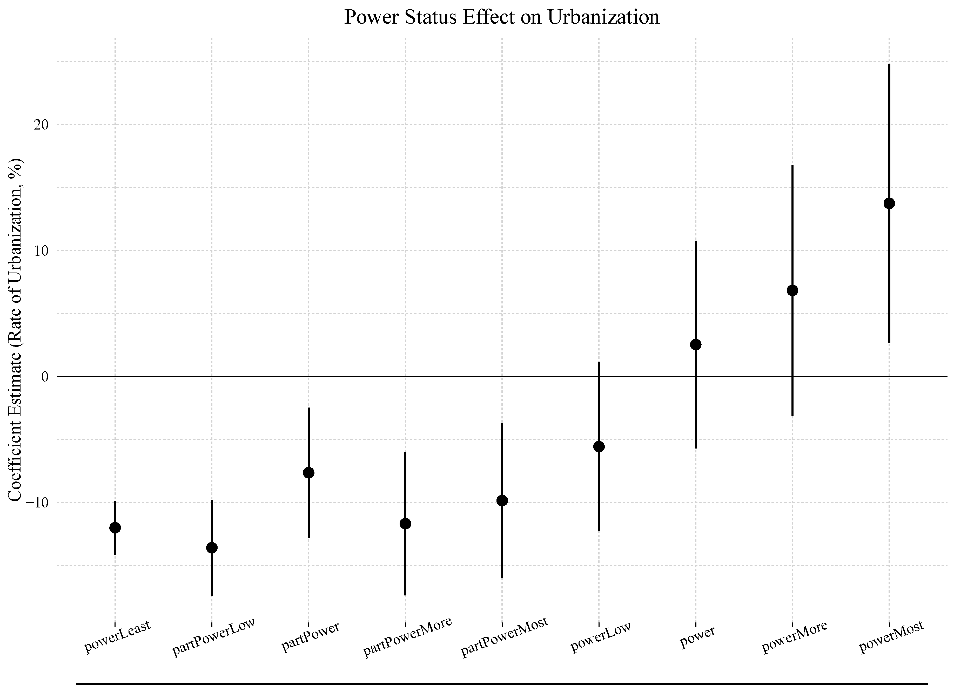
The interpretation of this graphic is that all powerStatus indicators from powerLeast to partPowerMost live in urban areas at statistically lower rates than their peers. By contrast, powerMost couples live in cities at statistically higher rates.
Appendix C Plot of Sample Fixed Effects
Figure A2 displays the fixed effects estimates for each of the four included as part of the fifth presented model in Table 6. This model included fixed effects for the state (ST), PUMA, Year (year), and jobTag. The value of zero on each panel of the plot represents the mean value for that fixed effect across all values, meaning non-zero values can be interpreted as below- or above-average values for a particular fixed effect. Unfortunately, the provided function in the package [46] does not allow for much customization, but it does neatly display the various values for fixed effects.
Maine (ST/FIPS code of 23) has the lowest fixed effect value while Rhode Island (ST/FIPS of 44) has the highest. These simply capture statewide urbanization effects that, when paired with PUMA effects fully capture urbanization trends geographically. These too appear distinct, with the built-in breaks in the plot representing all other PUMAs outside of the lowest and highest five.
Figure A2.
Fixed Effects Estimates – Ordered Ascending
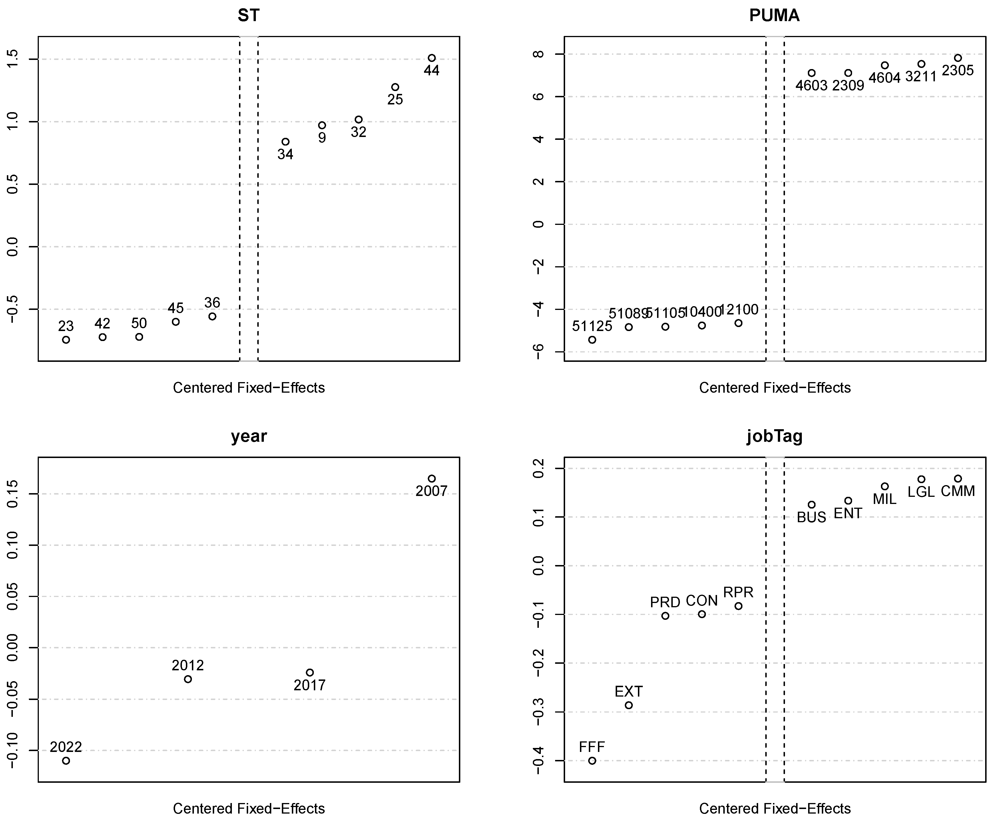
Unsurprisingly, 2007 has the highest year-based fixed effect given the noted downward trend in urbanization throughout this sample. Finally, there are significant differences in fixed effects for jobTag. On the low end, the tag FFF represents farming, fishing, and forestry, which is unsurprisingly performed by individuals unlikely to live in urban areas. In the middle, occupations like PRD – production or manufacturing jobs – seem distinct from occupations typically linked with urban areas such as legal jobs (LGL) or entertainment (ENT). All told, the graphic provides evidence in a very simple way that there are differences across fixed effects.
References
- Artz, G. Rural area brain drain: Is it a reality? Choices 2003, 18, 11–15. [Google Scholar]
- Waldorf, B.S. Brain Drain in Rural America 2007.
- Carr, P.J.; Kefalas, M.J. Hollowing out the middle: The rural brain drain and what it means for America; Beacon press, 2009.
- Carr, P.J.; Kefalas, M.J. The rural brain drain. The Chronicle of Higher Education 2009, 9, 1–13. [Google Scholar]
- Sherman, J.; Sage, R. Sending Off All Your Good Treasures: Rural Schools, Brain-Drain, and Community Survival in the Wake of Economic Collapse. Journal of Research in Rural Education 2011, 26. [Google Scholar]
- Estes, H.K.; Estes, S.; Johnson, D.M.; Edgar, L.D.; Shoulders, C.W. The rural brain drain and choice of major: Evidence from one land grant university. NACTA Journal 2016, 60, 9–13. [Google Scholar]
- Vazzana, C.M.; Rudi-Polloshka, J. Appalachia has got talent, but why does it flow away? A study on the determinants of brain drain from rural USA. Economic Development Quarterly 2019, 33, 220–233. [Google Scholar]
- Costa, D.L.; Kahn, M.E. Power couples: changes in the locational choice of the college educated, 1940–1990. The Quarterly Journal of Economics 2000, 115, 1287–1315. [Google Scholar] [CrossRef]
- Berliant, M.; Fujita, M. The dynamics of knowledge diversity and economic growth. Southern Economic Journal 2011, 77, 856–884. [Google Scholar]
- Ager, P.; Brückner, M. Cultural diversity and economic growth: Evidence from the US during the age of mass migration. European Economic Review 2013, 64, 76–97. [Google Scholar]
- Gören, E. How ethnic diversity affects economic growth. World Development 2014, 59, 275–297. [Google Scholar]
- Bove, V.; Elia, L. Migration, diversity, and economic growth. World Development 2017, 89, 227–239. [Google Scholar] [CrossRef]
- Ritchie, H.; Roser, M. Urbanization. Our World in Data 2018. https://ourworldindata.org/urbanization.
- Sato, Y.; Yamamoto, K. Population concentration, urbanization, and demographic transition. Journal of Urban Economics 2005, 58, 45–61. [Google Scholar] [CrossRef]
- Hofmann, A.; Wan, G. Determinants of Urbanization 2013. hdl:11540/2310.
- Glaeser, E.L.; Gottlieb, J.D. The wealth of cities: Agglomeration economies and spatial equilibrium in the United States. Journal of economic literature 2009, 47, 983–1028. [Google Scholar]
- Jacobs, J. The Economy of Cities; Random House, 1969.
- Simon, C.J. Migration and career attainment of power couples: the roles of city size and human capital composition. Journal of Economic Geography 2019, 19, 505–534. [Google Scholar]
- Greenwood, M.J. Research on Internal Migration in the United States: A Survey. Journal of Economic Literature 1975, 13, 397–433. [Google Scholar]
- Basker, E. Education, Job Search and Migration. University of Missouri-Columbia Working Paper 2002, pp. 02–16.
- Clark, T.; Lloyd, R.; Wong, K.; Jain, P. Amenities Drive Urban Growth. Journal of Urban Affairs 2002, 24, 493–515. [Google Scholar]
- Bernard, A.; Bell, M. Educational selectivity of internal migrants: A global assessment. Demographic research 2018, 39, 835–854. [Google Scholar]
- Schwartz, A. Migration and Life Span Earnings in the U.S. PhD thesis, University of Chicago, 1968.
- Parker, K.; Menasce Horowitz, J.; Brown, A.; Fry, R.; Cohn, D.; Igielnik, R. Demographic and economic trends in urban, suburban and rural communities. Pew Research Center, 2018.
- Backman, M. Returns to Education across the urban-rural hierarchy. The Review of Regional Studies 2014, 44, 33–59. [Google Scholar]
- Chen, Y.; Rosenthal, S.S. Local amenities and life-cycle migration: Do people move for jobs or fun? Journal of Urban Economics 2008, 64, 519–537. [Google Scholar]
- Lee, M. Losing Our Mind: Brain Drain across the United States. SCP REPORT NO. 2-19, 2019.
- Vazzana, C.M.; Rudi-Polloshka, J. Appalachia Has Got Talent, But Why Does It Flow Away? A Study on the Determinants of Brain Drain From Rural USA. Economic Development Quarterly 2019, 33, 220–233. [Google Scholar] [CrossRef]
- Jeworrek, S.; Brachert, M. Are rural firms left behind? Firm location and perceived job attractiveness of high-skilled workers. Cambridge Journal of Regions, Economy and Society 2024, 17, 75–86. [Google Scholar] [CrossRef]
- Miller, J.C.; Collins, S. what is the economic impact of "brain drain" in Mississippi? University Research Center Mississippi Institutions of Higher Learning, 2022.
- Economic Innovation Group, R. The New Map of Economic Growth and Recovery. Economic Innovation Group, 2016.
- Isaac, J. Economics of Migration; Oxford University Press, 1947.
- Rusconi, Alessandra Solga, H. A Systematic Reflection upon Dual Career Couples. Social Science Research Center Berlin 2008.
- Rabe, B. Dual-earner migration. Earnings gains, employment and self-selection. Journal of Population Economics 2011, 24, 477–497. [Google Scholar]
- Becker, P.E.; Moen, P. Scaling back: Dual-earner couples’ work-family strategies. Journal of Marriage and the Family, 1007. [Google Scholar]
- Wolf-Wendel, L.E. Dual-Career Couples: Keeping Them Together. The Journal of Higher Education 2000, 71, 291–321. [Google Scholar] [CrossRef]
- Boyle, P.; Feng, Z.; Gayle, V. A New Look at Family Migration and Women’s Employment Status. Journal of Marriage and Family 2009, 71, 417–431. [Google Scholar]
- Boyle, P.; J. , C.T.; Halfacree, K.; Smith, D. A Cross-National Comparison of the Impact of Family Migration on Women’s Employment Status. Demography 2001, 38, 201–213. [Google Scholar]
- Lee, S.; Roseman, C.C. Migration determinants and employment consequences of white and black families, 1985–1990. Economic Geography 1999, 75, 109–133. [Google Scholar]
- Jayachandran, S.; Nassal, L.; Notowidigdo, M.J.; Paul, M.; Sarsons, H.; Sundberg, E. Moving to Opportunity, Together. Working Paper 32970, National Bureau of Economic Research, 2024. [CrossRef]
- Venator, J. Concentrating on His Career or Hers?: Descriptive Evidence on Occupational Co-agglomeration in Dual-Earner Households. PhD thesis, Boston College, 2024.
- Compton, J.; Pollak, R.A. Why are power couples increasingly concentrated in large metropolitan areas? Journal of Labor Economics 2007, 25, 475–512. [Google Scholar]
- Missouri Census Data Center. Geocorr Applications, 2025.
- William Revelle. psych: Procedures for Psychological, Psychometric, and Personality Research. Northwestern University, Evanston, Illinois, 2023. R package version 2.3.9.
- U.S. Census Bureau. COMMUTING CHARACTERISTICS BY SEX. U.S. Census Bureau, 2021. Accessed on 26 February 2025.
- Bergé, L. Efficient estimation of maximum likelihood models with multiple fixed-effects: the R package FENmlm. CREA Discussion Papers 2018. [Google Scholar]
| 1 | For a longer review of the agglomeration effects, innovation, and employment growth, see [17]. |
| 2 | The phenomenon by which highly educated individuals move to urban areas, reducing the ability of rural labor markets to retain employment opportunities for skilled workers in the long run. |
| 3 | We use 5-year samples for all years besides 2007, which only had 3-year samples available. |
| 4 | For this analysis, the data, visuals, and regressions alone required 200+ GB of computer RAM, very near the upper limit of technology available to the authors. |
| 5 | Some households are multi-family, which means more than two married couples live in the home. Because we do not know how these individuals are partnered, we classify them differently and eventually treat them as no different from unmarried individuals. We do the same for individuals that report being married, but are living alone. The rationale behind the former is simply based on the constraints of the data, while the rationale for the latter is that it is unlikely a married individual living alone would make the joint-migration decision we are investigating. |
| 6 | PUMAs divide the entirety of the United States into parcels that consist of more than 100,000 persons. |
| 7 | For robustness, we tried alternative definitions that defined urban areas using 75% and 80% as the delineation but neither meaningfully changed the results. |
| 8 | A full set of powerStatus summary statistics can be found in Appendix A. |
| 9 | Theoretically urban areas can change over time, though that change is minimal over the course of our four year sample. |
Table 1.
Primary Variables Used from the PUMS Data
| Variable | Description | Use |
|---|---|---|
| MAR | Marital Status | Used to identify individuals as married or unmarried |
| PUMA | FIPS PUMA Code | Used to identify PUMA (location) of individual |
| RAC1P | Racial Category | Used to identify self-reported race of individual and partner |
| SCHL | Educational Attainment | Used to identify highest degree earned for person and their partner |
| SERIALNO | Household Identifier | Used to pair potential partners living in the same home |
| SEX | Sex of person | Used to identify couple type (e.g. heterosexual, same sex) |
| ST | FIPS State Code | Used to identify state (location) of individual |
Table 2.
Possible Categories for Individuals and Couples
| Single Individuals | Couples | |||
|---|---|---|---|---|
| Characteristic | Variable(s) Used | Possible Values | Variable(s) Used | Possible Values |
| Power Designation (powerStatus) |
SCHL | Varies by PUMS year | SCHL MAR |
powerLeast partPowerLow partPower partPowerMore partPowerMost powerLow power powerMore powerMost |
| Couple Type (copType) |
MAR | single | MAR SEX |
female-female (FF) female-male (FM) male-male (MM) |
| Race (raceStatus) |
RAC1P | White Black/African American American Indian Alaska Native American Indian/Alaska Native Asian Native Hawaiian/Pacific Islander Some other race Two or more major races |
RAC1P MAR |
asian black mixed other white |
| Labor Force Status (laborStatus) |
ESR WORKSTAT OCCP |
Codes indicating labor force status Code for individual’s occupation (jobTag) |
MAR FES OCCP |
bothLF oneLF noLF |
Italicized values represent how variables are stored and these terms are used frequently throughout the rest of the paper. Power designations are ordered by educational attainment, from least to most. powerLeast is assigned to couples for which both partners have attained no more than a high school education; partPowerLow is assigned to couples for which one partner has attended some college, but not yet earned a bachelor’s degree; powerLow is analogous, but assigned when both partners have completed some college, and so on. For multi-family and solo married households, we argue the co-location effect is relatively weak as compared to single-family households. For a married person living alone (without a partner in the house), the rationale behind omitting these groupings is strong. Presumably, any co-location effect would be weaker for such couples as compared to those that co-habitate. Couples are defined as asian, black, or whiteif both members of the couple fit that racial category. mixed is assigned to couples that self-identify as split race couples (e.g. one individual is black and one is white) and those who both self identify as “Two or more major races" in the PUMS survey. other represents all other couples that do not fit in the the other categories and saved for prospective future work. Labor force status assigns a code to each married couple indicating whether both were labor force participants (bothLF), only one was a labor force participant (oneLF), or neither was a labor force participant (noLF). This allows this study to match previous work that focuses on dual income-earning households while investigating if the results hold for others.
Table 3.
Select Urbanization Rate Summary Statistics for 2007 to 2022–Grouped by Power Category
| 2007 | 2012 | 2017 | 2022 | ||||||
|---|---|---|---|---|---|---|---|---|---|
| Category | Variable | n | mean (sd) |
n | mean (sd) |
n | mean (sd) |
n | mean (sd) |
| powerLeast | urb | 1,032,208 | 48.96 (49.99) |
295,536 | 51.96 (49.96) |
1,351,934 | 52.78 (49.92) |
157,426 | 49.55 (50.00) |
| urbPro | 1,032,208 | 68.19 (27.31) |
295,536 | 70.01 (27.61) |
1,351,934 | 70.49 (27.53) |
157,426 | 68.80 (27.62) |
|
| partPower | urb | 204,982 | 60.64 (48.85) |
66,604 | 62.33 (48.46) |
354,552 | 63.47 (48.15) |
51,330 | 57.11 (49.49) |
| urbPro | 204,982 | 74.90 (25.43) |
66,604 | 75.93 (25.75) |
354,552 | 76.58 (25.51) |
51,330 | 73.41 (26.55) |
|
| power | urb | 285,918 | 72.33 (44.73) |
98,076 | 75.24 (43.16) |
529,668 | 75.79 (42.84) |
75,542 | 69.33 (46.11) |
| urbPro | 285,918 | 81.46 (22.51) |
98,076 | 83.32 (22.42) |
529,668 | 83.57 (22.17) |
75,542 | 80.47 (24.19) |
|
| powerMost | urb | 34,418 | 82.18 (38.27) |
12,926 | 84.22 (36.46) |
75,952 | 84.11 (36.56) |
10,938 | 79.30 (40.52) |
| urbPro | 34,418 | 87.34 (19.43) |
12,926 | 88.45 (19.45) |
75,952 | 88.56 (19.26) |
10,938 | 86.25 (21.40) |
|
n represents the number of observations (people that are a part of a couple) that match this categorical definition in the sample. mean and standard deviation (sd) represent summary statistics for urbanization rates for each demographic, based on how urban status is defined.
Table 4.
Select Urbanization Rate Summary Statistics for 2007 to 2022–Grouped by Couple Sexual Orientation
Table 4.
Select Urbanization Rate Summary Statistics for 2007 to 2022–Grouped by Couple Sexual Orientation
| 2007 | 2012 | 2017 | 2022 | ||||||
|---|---|---|---|---|---|---|---|---|---|
| Category | Variable | n | mean (sd) |
n | mean (sd) |
n | mean (sd) |
n | mean (sd) |
| Heterosexual (FM) | urb | 3,720,536 | 58.89 (49.20) |
1,219,180 | 61.81 (48.59) |
6,133,590 | 62.82 (48.33) |
800,502 | 58.14 (49.33) |
| urbPro | 3,720,536 | 73.88 (25.90) |
1,219,180 | 75.62 (26.08) |
6,133,590 | 76.18 (25.86) |
800,502 | 73.88 (26.61) |
|
| Same-sex (FF) | urb | 2,078 | 75.26 (43.16) |
736 | 78.26 (41.28) |
28,362 | 71.55 (45.12) |
5,158 | 68.24 (46.56) |
| urbPro | 2,078 | 83.26 (23.65) |
736 | 85.85 (21.49) |
28,362 | 81.47 (24.29) |
5,158 | 79.94 (24.98) |
|
| Same-sex (MM) | urb | 4,340 | 76.54 (42.38) |
926 | 80.56 (39.59) |
27,654 | 77.12 (42.01) |
4,940 | 76.23 (42.57) |
| urbPro | 4,340 | 84.49 (23.39) |
926 | 86.59 (22.11) |
27,654 | 84.73 (22.55) |
4,940 | 84.69 (22.84) |
|
n represents the number of observations (people that are a part of a couple) that match this categorical definition in the sample. mean and standard deviation (sd) represent summary statistics for urbanization rates for each demographic, based on how urban status is defined.
Table 5.
Select Urbanization Rate Summary Statistics for 2007 to 2022–Grouped by Couple Racial Status
Table 5.
Select Urbanization Rate Summary Statistics for 2007 to 2022–Grouped by Couple Racial Status
| 2007 | 2012 | 2017 | 2022 | ||||||
|---|---|---|---|---|---|---|---|---|---|
| n | mean (sd) |
n | mean (sd) |
n | mean (sd) |
n | mean (sd) |
||
| asian | urb | 125,332 | 93.37 (24.87) |
48,506 | 95.28 (21.20) |
264,544 | 95.53 (20.67) |
37,940 | 93.78 (24.15) |
| urbPro | 125,332 | 94.32 (12.55) |
48,506 | 95.71 (11.46) |
264,544 | 95.80 (10.96) |
37,940 | 94.86 (12.57) |
|
| black | urb | 189,864 | 73.52 (44.12) |
65,810 | 77.41 (41.82) |
318,678 | 77.75 (41.59) |
34,068 | 71.50 (45.14) |
| urbPro | 189,864 | 82.46 (24.45) |
65,810 | 84.35 (23.72) |
318,678 | 84.52 (23.42) |
34,068 | 81.48 (24.87) |
|
| mixed | urb | 201,134 | 71.38 (45.20) |
70,124 | 74.46 (43.61) |
388,494 | 75.46 (43.03) |
97,254 | 69.85 (45.89) |
| urbPro | 201,134 | 81.08 (23.27) |
70,124 | 82.89 (23.22) |
388,494 | 83.45 (22.95) |
97,254 | 80.85 (24.08) |
|
| white | urb | 3,081,674 | 54.87 (49.76) |
1,001,136 | 57.76 (49.39) |
5,035,466 | 58.71 (49.23) |
568,834 | 50.42 (50.00) |
| urbPro | 3,081,674 | 71.54 (26.03) |
1,001,136 | 73.24 (26.31) |
5,035,466 | 73.77 (26.14) |
568,834 | 69.34 (26.87) |
|
n represents the number of observations (people that are a part of a couple) that match this categorical definition in the sample. mean and standard deviation (sd) represent summary statistics for urbanization rates for each demographic, based on how urban status is defined. A person receives the tag asian only if their spouse also has the `Asian’ code for RAC1P in the PUMS data. The same goes for the other displayed categories except for: mixed – which is a tag assigned to an individual that is married to a person with a different racial code.
Table 6.
Fixed Effects Regression Results for Differential Urbanization Rates by Power Status
| Dependent Variables: | urbPro | urb | urbPro | urb | ||
| Model: | (1) | (2) | (3) | (4) | (5) | (6) |
| WLS | Logit | WLS | Logit | Logit | Logit | |
| Variables | ||||||
| powerLeast | -0. | -0. | -0. | -0. | -0. | -0. |
| (0.000) | (0.007) | (0.001) | (0.013) | (0.011) | (0.028) | |
| partPower | -0. | -0. | -0. | -0. | -0. | -0. |
| (0.001) | (0.002) | (0.001) | (0.006) | (0.026) | (0.058) | |
| partPowerLow | -0. | -0. | -0. | -0. | -0. | -0. |
| (0.001) | (0.004) | (0.001) | (0.006) | (0.019) | (0.046) | |
| partPowerMore | -0. | -0. | -0. | -0. | -0. | -0. |
| (0.001) | (0.002) | (0.001) | (0.006) | (0.029) | (0.064) | |
| partPowerMost | -0. | -0. | -0. | -0. | -0. | -0. |
| (0.001) | (0.003) | (0.001) | (0.008) | (0.031) | (0.068) | |
| power | 0. | 0. | 0. | 0. | 0.025 | 0.075 |
| (0.001) | (0.009) | (0.002) | (0.016) | (0.042) | (0.085) | |
| powerLow | -0. | -0. | -0. | -0. | -0.056 | -0.116 |
| (0.001) | (0.005) | (0.002) | (0.010) | (0.034) | (0.072) | |
| powerMore | 0. | 0. | 0. | 0. | 0.068 | 0.161 |
| (0.001) | (0.010) | (0.002) | (0.016) | (0.051) | (0.101) | |
| powerMost | 0. | 0. | 0. | 0. | 0. | 0. |
| (0.001) | (0.012) | (0.002) | (0.020) | (0.056) | (0.109) | |
| Fixed-effects | ||||||
| State | Yes | Yes | Yes | Yes | Yes | Yes |
| PUMA | Yes | Yes | Yes | Yes | Yes | Yes |
| Year | Yes | Yes | Yes | Yes | Yes | Yes |
| Occupational Code | Yes | Yes | ||||
| Fit statistics | ||||||
| Observations | 28,812,792 | 25,760,965 | 28,812,792 | 17,362,455 | 12,502,105 | 8,382,183 |
| Squared Correlation | 0.66487 | 0.64727 | 0.59257 | 0.40297 | 0.64282 | 0.40621 |
| Pseudo | 0.52746 | 0.78225 | 0.98474 | 0.32397 | 0.78209 | 0.32620 |
Coefficients are interpreted as percentages. For the coefficient on powerMost from the first column, the coefficient would imply that two married partners with doctoral or professional degrees are 0.013% more likely to live in urban environments than their otherwise equal peers. Controls included are age, sex, educational attainment, and racial code, though those coefficients are not included in the table. Standard errors are clustered by power status Significance Codes are: ***: 0.01, **: 0.05, *: 0.1.
Table 7.
Fixed Effects Regression Results for Differential Urbanization Rates by Sexual Orientation (copType)
Table 7.
Fixed Effects Regression Results for Differential Urbanization Rates by Sexual Orientation (copType)
| Dependent Variable: | urbPro | |||||
| Model: | (1) | (2) | (3) | (4) | (5) | (6) |
| FF | FM | MM | FF | FM | MM | |
| Variables | ||||||
| powerLeast | -0. | -0. | 0. | -0. | 0. | 0. |
| (0.007) | (0.000) | (0.000) | (0.011) | (0.000) | (0.000) | |
| partPowerLow | -0. | -0. | 0. | -0. | -0. | 0. |
| (0.004) | (0.000) | (0.000) | (0.003) | (0.000) | (0.000) | |
| partPower | -0. | 0. | 0. | -0. | -0. | 0. |
| (0.002) | (0.000) | (0.000) | (0.006) | (0.000) | (0.000) | |
| partPowerMore | -0. | -0. | 0. | -0. | -0. | 0. |
| (0.002) | (0.000) | (0.000) | (0.009) | (0.000) | (0.000) | |
| partPowerMost | -0. | 0. | -0. | -0. | 0. | -0. |
| (0.003) | (0.000) | (0.000) | (0.011) | (0.000) | (0.000) | |
| power | 0. | 0. | 0. | -0.016 | -0. | -0. |
| (0.009) | (0.000) | (0.000) | (0.021) | (0.000) | (0.000) | |
| powerLow | -0. | -0. | 0. | -0. | -0. | -0. |
| (0.005) | (0.000) | (0.000) | (0.013) | (0.000) | (0.000) | |
| powerMore | 0. | 0. | -0. | 0.028 | -0. | -0. |
| (0.010) | (0.000) | (0.000) | (0.030) | (0.000) | (0.000) | |
| powerMost | 0. | 0. | -0. | 0. | -0. | -0. |
| (0.012) | (0.000) | (0.000) | (0.036) | (0.000) | (0.001) | |
| Fixed-effects | ||||||
| State | Yes | Yes | Yes | Yes | Yes | Yes |
| PUMA | Yes | Yes | Yes | Yes | Yes | Yes |
| Year | Yes | Yes | Yes | Yes | Yes | Yes |
| Occupational Code | Yes | Yes | Yes | |||
| Fit statistics | ||||||
| Observations | 25,699,279 | 14,878,939 | 14,878,801 | 12,462,182 | 7,146,752 | 7,146,659 |
| Squared Correlation | 0.64718 | 0.64465 | 0.64468 | 0.64268 | 0.64116 | 0.64123 |
| Pseudo | 0.78226 | 0.78217 | 0.78218 | 0.78210 | 0.78133 | 0.78135 |
Coefficients are interpreted as percentages. All models reported are estimated under using binomial logit regressions. For the coefficient on powerMost from the first column, the coefficient would imply that two married partners with doctoral or professional degrees are 0.16% more likely to live in urban environments than their otherwise equal peers. Controls included are age, sex, educational attainment, and racial code, though those coefficients are not included in the table. The last three columns labeled “bothInLF" isolates couples wherein both partners reported being in the labor force and compares them with otherwise equal single peers. In these specifications, controls for the occupation are included. Standard errors are clustered by power status Significance Codes are: ***: 0.01, **: 0.05, *: 0.1.
Table 8.
Fixed Effects Regression Results for Differential Urbanization Rates by Race Status (raceStatus)
Table 8.
Fixed Effects Regression Results for Differential Urbanization Rates by Race Status (raceStatus)
| Dependent Variable: | urbPro | |||||||
| Model: | asian | black | mixed | white | asian | black | mixed | white |
| Variables | ||||||||
| powerLeast | 0. | 0. | -0. | -0. | 0. | 0. | -0. | -0. |
| (0.003) | (0.007) | (0.010) | (0.010) | (0.003) | (0.006) | (0.011) | (0.011) | |
| partPowerLow | 0. | 0. | -0. | -0. | 0. | 0. | -0. | -0. |
| (0.001) | (0.006) | (0.010) | (0.007) | (0.001) | (0.007) | (0.012) | (0.005) | |
| partPower | 0. | 0. | -0. | -0. | 0. | 0. | -0. | -0. |
| (0.002) | (0.006) | (0.009) | (0.005) | (0.002) | (0.007) | (0.013) | (0.003) | |
| partPowerMore | 0. | 0. | -0. | -0. | 0. | 0. | -0. | -0. |
| (0.003) | (0.006) | (0.010) | (0.005) | (0.002) | (0.007) | (0.013) | (0.005) | |
| partPowerMost | 0. | 0. | 0.012 | -0. | 0. | 0. | -0. | -0. |
| (0.001) | (0.007) | (0.009) | (0.005) | (0.000) | (0.008) | (0.012) | (0.008) | |
| powerLow | 0. | 0. | -0. | -0. | 0. | 0. | -0. | -0. |
| (0.001) | (0.005) | (0.009) | (0.003) | (0.001) | (0.007) | (0.013) | (0.008) | |
| power | 0. | 0. | 0. | 0. | 0. | 0. | -0.016 | -0. |
| (0.002) | (0.005) | (0.010) | (0.006) | (0.001) | (0.007) | (0.014) | (0.016) | |
| powerMore | 0. | 0. | 0. | 0. | 0. | 0. | -0.003 | 0.003 |
| (0.000) | (0.004) | (0.009) | (0.007) | (0.002) | (0.008) | (0.015) | (0.025) | |
| powerMost | 0. | 0. | 0. | 0. | 0. | 0. | 0. | 0. |
| (0.000) | (0.003) | (0.009) | (0.011) | (0.001) | (0.006) | (0.016) | (0.031) | |
| Fixed-effects | ||||||||
| State | Yes | Yes | Yes | Yes | Yes | Yes | Yes | Yes |
| PUMA | Yes | Yes | Yes | Yes | Yes | Yes | Yes | Yes |
| Year | Yes | Yes | Yes | Yes | Yes | Yes | Yes | Yes |
| jobTag | Yes | Yes | Yes | Yes | ||||
| Fit statistics | ||||||||
| Observations | 15,214,227 | 15,369,645 | 15,509,493 | 23,885,857 | 7,316,751 | 7,389,236 | 7,498,483 | 11,525,695 |
| Squared Correlation | 0.64804 | 0.64464 | 0.64501 | 0.64445 | 0.64437 | 0.64110 | 0.64147 | 0.64004 |
| Pseudo | 0.78258 | 0.78187 | 0.78202 | 0.78251 | 0.78168 | 0.78114 | 0.78114 | 0.78243 |
Coefficients are interpreted as percentages. For the coefficient on powerMost from the first column, the coefficient would imply that two married partners with doctoral or professional degrees are 0.16% more likely to live in urban environments than their otherwise equal peers. Controls included are age, sex, educational attainment, and racial code, though those coefficients are not included in the table. The last three columns labeled “bothInLF" isolates couples wherein both partners reported being in the labor force and compares them with otherwise equal single peers. In these specifications, controls for the occupation are included. Standard errors are clustered by power status Significance Codes are: ***: 0.01, **: 0.05, *: 0.1.
Disclaimer/Publisher’s Note: The statements, opinions and data contained in all publications are solely those of the individual author(s) and contributor(s) and not of MDPI and/or the editor(s). MDPI and/or the editor(s) disclaim responsibility for any injury to people or property resulting from any ideas, methods, instructions or products referred to in the content. |
© 2025 by the authors. Licensee MDPI, Basel, Switzerland. This article is an open access article distributed under the terms and conditions of the Creative Commons Attribution (CC BY) license (http://creativecommons.org/licenses/by/4.0/).
Copyright: This open access article is published under a Creative Commons CC BY 4.0 license, which permit the free download, distribution, and reuse, provided that the author and preprint are cited in any reuse.


